Compressed Spectrum Sensing in the Presence of ... - IEEE Xplore

COMPRESSED SPECTRUM SENSING IN THE PRESENCE OF INTERFERENCE: COMPARISON OF SPARSE RECOVERY STRATEGIES Eva Lagunas and Montse Nájar Department of Signal Theory and Communications, Universitat Politècnica de Catalunya (UPC), Barcelona, Spain Email: {eva.lagunas,montse.najar}@upc.edu ABSTRACT Existing approaches to Compressive Sensing (CS) of sparse spectrum has thus far assumed models contaminated with noise (either bounded noise or Gaussian with known power). In practical Cognitive Radio (CR) networks, primary users must be detected even in the presence of low-regulated transmissions from unlicensed systems, which cannot be taken into account in the CS model because of their non-regulated nature. In [1], the authors proposed an overcomplete dictionary that contains tuned spectral shapes of the primary user to sparsely represent the primary users’ spectral support, thus allowing all frequency location hypothesis to be jointly evaluated in a global unified optimization framework. Extraction of the primary user frequency locations is then performed based on sparse signal recovery algorithms. Here, we compare different sparse reconstruction strategies and we show through simulation results the link between the interference rejection capabilities and the positive semidefinite character of the residual autocorrelation matrix. Index Terms— Spectrum Sensing, Compressive Sensing, Interference Mitigation, Cognitive Radio 1. INTRODUCTION TO THE SPECTRUM SENSING PROBLEM The basic idea of Cognitive Radio (CR) is spectral reusing or spectrum sharing, which allows the unlicensed users to communicate over licensed spectrum when the licensed holders are not fully utilizing it [2]. In this context, the main goal of spectrum sensing is to decide whether a given frequency band is occupied by a primary user or not based on the observation of the received signal [3]. Let us denote x(t) the wideband signal representing the superposition of different primary systems in a CR network. Signal x(t) is assumed to be sparse This work was partially supported by the Spanish Ministry of Science and Innovation (Ministerio de Ciencia e Innovación) under project TEC201129006-C03-02 (GRE3N-LINK-MAC), by the European Commission in the framework of the FP7 Network of Excellence in Wireless COMmunications NEWCOM# (Grant agreement no. 318306), by the Catalan Government under grant 2009 SGR 891 and by the European Cooperation in Science and Technology under project COST Action IC0902.

1721

multiband signal, i.e, a bandlimited, continuous-time, squared integrable signal that has all of its energy concentrated in a small number of disjoint frequency bands. In other words, its spectral support has Lebesgue measure small relative to the overall signal bandwidth [4]. Denoting the Fourier transform of x(t) as X(f ), the spectral support of the multiband signal x(t), denoted as F ⊂ [0, fmax ], namely X(f ) = 0, f ∈ / F, is restricted to have its signal energy distributed on no more than Nb disjoint bands in F: F=

Nb [

[ai , bi )

(1)

i=1

where [ai , bi ), i = 1, . . . , Nb , represent the edges of each band. The spectral occupancy Ω is defined as, Ω=

λ(F ) fmax

0≤Ω≤1

(2)

where λ(F ) is the Lebesgue measure of the frequency set F , PNb (bi − ai ). In which, in this particular case, is equal to i=1 the spectrum sensing framework, the spectral support F is unknown but the total bandwidth under study is assumed to be sparse, i.e., Ω 6 1. The received signal y(t) consists on the superposition of multiple primary and secondary (interference) services. The non-regulated activity of the spectrum will be denoted as i(t) and henceforth is considered interference. The problem of determining whether a given frequency is occupied or not by a licensed radio can be modeled into a binary hypothesis test, ( i(t) + η(t) (H0 ) y(t) = (3) x(t) + i(t) + η(t) (H1 ) where (H0 ) stands for the absence of primary signal and (H1 ) represents the presence of a primary signal in the frequency channel under study. η(t) is AWGN, N (0, ση2 ). The interference i(t) is independent of the noise and primary signal, and we assume that its spectral shape is different from that of the primary. In practice, the secondary user is rarely going to use the same modulation as the primary. Moreover, the secondary

user generally transmits at a lower rate than the primary in order to not disturb the quality of service of the primary user. Therefore, and as a baseline, it is assumed throughout this section that the interference has smaller bandwidth than that of the primary. The presence of unknown interference, which has not been addressed in conventional spectrum sensing publications, adds additional challenges to the spectrum sensing problem. Note that information on primary users activity may potentially be used by the three relevant cognitive paradigms, namely interweave, underlay and overlay [5]. Let B denote the set of possible primary users’ frequency M −1 locations and let {ωm }m=0 denote a grid that covers B. Assuming that the true location of the primary users lie on the grid, the received signal y(t) can be rewritten as, y(t) =

M −1 X

x(t, ωm ) + i(t) + η(t)

where x(t, ωm ) denotes the analytic representation of the primary user corresponding to ωm , which is given by, (5)

where am (t) indicates the complex envelope of the source at ωm . Note that only a few am (t) are different from zero. For the sake of simple notation, we are assuming linear propagation channel with no distortion1 . 2. COMPRESSIVE SAMPLING The Compressive Sensing (CS) based candidate detector presented by the authors in [1] makes the assumption that only a small number of primary users exists and therefore only few grid points are occupied, i.e., denoting K the number of primary users present in y(t), K 0 is a suitable integer, i = 1, 2, . . . , κ and n ∈ Z. The set {ci } contains κ distinct integers chosen from {0, 1, . . . , L − 1}. The MC sampling process can be viewed as a classical Nyquist sampling followed by a block that discards all but κ samples in every block of L samples periodically. Thus, a sequence or coset of equally-spaced samples is obtained for each ci . The period of each one of these sequences is equal to LT . Therefore, one possible implementation consists of κ parallel ADCs, each working uniformly with period LT . 1 The

robustness in front of a frequency selective channel, instead of flat fading, have been studied in [6]

1722

3. CS-BASED SPECTRUM SENSING VIA SPECTRAL SHAPE FEATURE DETECTION This section reviews the CS-based spectral shape detector proposed in [1]. It is assumed that the primary signal x(t) is unknown, i.e., the transmitted symbols are not known a priori. For such a case, it is appropriate to define a secondorder based detector. To do so, the spectrum characteristics of the primary signals, which can be obtained by identifying its transmission technologies, are used as features. The basic strategy of the candidate detector is to compare the a priori known spectral shape of the primary user with the power spectral density of the received signal. To avoid the power spectral density computation of the received signal, the comparison is made in terms of autocorrelation by means of a correlation matching. The diagram of the CR receiver is sketched in Fig. 1.

Sub−Nyquist Sampling

Correlation Estimation

CS−based correlation matching

Fig. 1. Block diagram of the cognitive receiver

Firstly, taking advantage of the sparsity of the primary user’s signal spectrum, a sub-Nyquist sampling is used to overcome the problem of high sampling rate. Then, the compressed samples are processed in the autocorrelation estimation stage and finally, the correlation-matching based spectrum sensing is performed using a predetermined spectral shape, which has to be known a priori. Following the noˆ y ∈ Cκ×κ tation of (8), the sample autocorrelation matrix R can be obtained as, Nf X ˆy = 1 yf yH R f Nf f =1

(9)

For the purpose of the present work, let us define Rb as baseband candidate autocorrelation of the primary system. The expression of Rb is linked to the PSD of the primary system, which, for linearly modulated signals, depends mainly on the transmission rate and the modulation pulse. The aforementioned characteristics can be analytically extracted from physical layer standardization of primary services. In order to obtain the frequency location of each primary user, Rb is modulated by a rank-one matrix formed by the steering frequency vector at the sensed frequency ωm as follows, Rc (ωm ) = Rb e(ωm )eH (ωm ) (10) where denotes the elementwise product of two matrices and T e(ωm ) = 1 ejωm . . . ej(L−1)ωm is the steering vector. According to this notation, the corresponding model for the sample autocorrelation matrix defined in (9) is given by, ˆy = R

M −1 X

γ(ωm )ΦRc (ωm )ΦH + R

Conventional l1 -norm optimization can be applied to the reduced number of observations to recover the positions of primary users, min kˆry − Apkl2 + λ kpkl1 p≥0

(CONV)

P where kpkl1 = m |p(ωm )| and λ is the regularization parameter that essentially controls the trade-off between the sparsity of the solution and its fidelity to the measurements. How to calculate the optimal λ is still an open problem. The l1 -minimization is a convex problem and can be solved using convex optimization techniques [8]. One important drawback of (CONV) is the difficulty on rejecting interference. The interference immunity is not achieved only using a dictionary of candidates because, although the primary signals’ spectral shape are assumed to be of different nature than that of the interference, they might not be orthogonal.

(11) 4.2. Weighted l1 -norm minimization

m=0

where R represents the contribution of the sub-Nyquistsampled interference and noise autocorrelation matrices and γ(ωm ) is the power level at frequency ωm . The model in (11) can be conveniently rewritten into a sparse notation as follows, ˆry = kron(Φ, Φ)BSp + r = Ap + r

4.1. Conventional l1 -norm minimization

(12)

where kron(·, ·) denotes the Kronecker product. Vector ˆry ∈ κ2 × 1 is formed by the concatenation of the columns of ˆ y . From now on, to clarify notation, the concatenation of R columns will be denoted with the operator vec(·). Therefore, ˆ y ). B contains the spectral information of the priˆry = vec(R mary signals and is defined as diag(rb ) where rb = vec(Rb ). Matrix S defines the frequency scanning grid, S = s(ω0 ) s(ω1 ) · · · s(ωM −1 ) (13) where s(ωm ) = vec(e(ωm )eH (ωm )). The variable r encompasses interference and noise contribution. Vector p = T p(ω0 ) p(ω1 ) · · · p(ωM −1 ) can be viewed as the output of an indicator function, whose elements different from zero correspond to the frequencies where the reference is present. Moreover, the values different from zero correspond to the power of each primary user that is present. This is, ( γ(ωk ) if ωm = ωk (H1 ) p(ωm ) = (14) 0 otherwise (H0 ) 4. SPARSE RECONSTRUCTION STRATEGIES The previous sparse formulation begs for the use of wellknown sparse reconstruction strategies. The aim of this paper is to compare different sparse reconstruction methods to recover the true primary users’ frequency location, i.e., the sparse vector p.

1723

Recently, the l1 -norm has been shown to penalize large coefficients to the detriment of smaller coefficients [9]. Weighted l1 -norm have been proposed to democratically penalize nonzero entries. A novel weighted l1 -norm minimization was recently introduced by the authors in [1] to monitor the primary user spectrum activity in CR. The proposed weights M −1 {wm }m=0 were derived based on the positive-semidefinite character of the residual error matrix R . Those weights were H ˆ −1 given by the maximum eigenvalue of R y (ΦRc (ωm )Φ ). M −1 Therefore, all the hypothesis {ωm }m=0 can be evaluated in a global unified convex optimization by solving the following problem, min p(ωm )≥0

kˆry − Apkl2 + λ kWpkl1

(P0) M −1

where W is the diagonal matrix with the weights {wm }m=0 on the diagonal and zeros elsewhere. The problem (P0) was solved in [1] using CS-based iterative reconstruction methods. Finding robust stopping criteria in iterative CS reconstruction algorithms is a long standing problem for which a solution does not exist for CS models corrupted by unknown interference. This problem is skipped in [1] by running the algorithm until an heuristically chosen stopping criterion is met. In so doing, the algorithm is forced to stop before any interference signal is included in the reconstructed data. In general, the existing CS algorithms are classified into two sorts: those based on greedy search, and those based on convex optimization. The latter, although generally with higher computational complexity, does not require the user to find robust stopping criteria. Therefore, in order to skip the tough stopping criteria of the iterative greedy algorithms, the optimization problem (P0) is solved here using LP.

15

4.3. Weighted and Constrained l1 -norm minimization

15

← 10.50 dB

10

← 10.09 dB

10

← 8.51 dB

← 8.44 dB 5

0 dB

0 dB

It was mentioned that preserving the positive-semidefinite character of the residual error matrix R significantly improves the interference rejection capabilities of the CS-based spectral shape detector. However, we will show on the simulations section that the weighted formulation of the 11 -norm minimization is not enough to not include the interference on the solution. For comparison purposes, let us consider the following unweighted and weighted l1 -norm minimization problems,

5

−5

−5

−10

−10

−15

−20

−15

0

0.2

0.4 0.6 Norm. Frequency

0.8

−20

1

kˆry − Apkl2 + λ kpkl1 M −1 X

10

10

← 8.90 dB

γ(ωm )ΦRc (ωm )Φ

(P1) 0

m=1

p(ωm )≥0

← 9.41 dB

dB

0

−5

← −7.69 dB −10

−10

−15

−15

−20

0

0.2


(c) min

1

5

0

H

0.8

(b)

−5

ˆy − s.t. R


15

dB

min

0.2

(a) 15

5

p(ωm )≥0

0

0.8

1

−20

← −10.67 dB

0

0.2


0.8

1

(d)

kˆry − Apkl2 + λ kWpkl1

ˆy − s.t. R

M −1 X

γ(ωm )ΦRc (ωm )Φ

H

(P2) 0

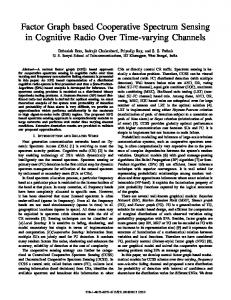
Fig. 2. CVX figures for ρ = 0.52: (a) CONV, (b) P0, (c) P1, and (d) P2.

m=1

where a restriction on the positive semi-definite character of the residual error matrix has been imposed. 5. SIMULATION RESULTS In this section, we evaluate the performance of the different sparsity-based reconstruction algorithms using synthesized data. The spectral band under scrutiny has bandwidth equal to fmax = 20 MHz. The size of the observation zf is L = 33 samples. The sampling rates of yf and zf are related through κ . To strictly focus on the perthe compression rate ρ = L formance behavior due to compression and remove the effect of insufficient data records, the size of the compressed observations is forced to be the same for any compression rate. Therefore, we set M = 2Lδρ−1 where δ is a constant (in the following results δ = 10). Thus, for a high compression rate, the estimator takes samples for a larger period of time. Note that the value of M determines the grid density of the spectrum to be scanned. Increasing M makes the grid finer, but it also increases the computational complexity. On the other hand, making the grid too rough might introduce substantial bias into the estimates. The grid resolution for this section is ∆ω = 100 kHz. The l1 -norm minimizations are solved with the convex optimization program CVX [10]. To test the ability of the reconstruction techniques to properly label licensed users, we have run 1000 Monte Carlo iterations (based on the noise randomness) of a scenario with one primary user in the presence of noise and interference. The interference is included as a 10 dB pure tone at normalized frequency 0.75, whereas the primary user is assumed to be a BPSK signal with a rectangular pulse shape and 8 samples

1724

per symbol. The SNR of the desired user is 10 dB and its normalized carrier frequency is 0.25. The spectral occupancy for this particular example is Ω = 0.25 (the primary user is using one quarter of the available spectrum). According to Landau’s lower bound [4], the minimum average sampling rate for most signals is given by the Nyquist rate multiplied by the spectral occupancy, which is often much lower than the corresponding Nyquist rate. For this particular example, Landau’s lower bound is telling us than 3 of every 4 Nyquist samples can be thrown away without affecting the signal reconstruction. The results shown next consider λ = 1 and ρ = 0.52, which corresponds to κ = 17 and M = 1281. Fig. 2 shows the average performance of the different CSbased reconstruction strategies presented in the previous section after 1000 Monte Carlo runs. Fig. 2(a) displays the conventional l1 -norm minimization, which is not robust to the strong interference. The use of the proposed weights helps in reducing the interference contribution, as shown in Fig. 2(b), but is not enough to discern between the primary user and the interference signal. The advantage of imposing positive semi-definite residual correlation matrix is evident from Figs. 2(c) and 2(d), where the difference between the peak corresponding to the true primary user and the peak corresponding to the interference has been significantly increased compared to Figs. 2(a) and 2(b). Moreover, we see from Fig. 2(d) a marked improvement over the unweighted l1 -norm reconstruction: the use of weights helps in reducing the interference level in 3dB. We would like to confirm the advantages of the weighted and constrained l1 -norm minimization (P2) over its competitors for compressible spectrum sensing. To do so, let us now

1 1 Histogram: Primary Histogram: Interference PDF Approx. PDF Approx.

0.8

0.6 Pd

0.6

0.8

0.4

CONV P0 P1 P2

0.4 0.2 0.2 0 0 −9

−8 −8

−7

−6

−5 −4 Test Statistic

−3

−2

−1

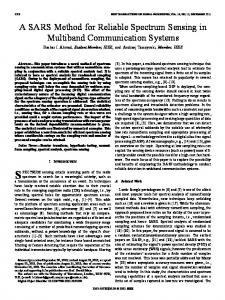
Fig. 3. Theoretical and empirical distributions of H1 and H0

for interference’s SNR = 7.5 dB and ρ = 0.52. evaluate the probability of detection (Pd ) versus SNR of the interference for the same scenario as before but with the primary user transmitting at SNR = 0dB. Theoretical derivation of a detection threshold to meet the required Pf a requires the statistical distribution of both H1 and H0, which is a difficult task, especially for functions resulting from optimization problems. To find an approximate distribution of H1 and H0, we recorded 4.000 Monte Carlo simulations, keeping the peak value of the true primary user frequency location (H1) and keeping the peak value corresponding to the interference (H0). Fig. 3 shows the normalized distributions of H0 and H1 for a particular example with interference’s SNR = 7.5 dB and ρ = 0.52 solving (P2). The approximated probability density function computed using a kernel smoothing method is also plotted in Fig. 3 and it is seen that both distributions closely match the nonparametric approximation. In view of the results, we decided to adopt nonparametric density estimates for the computation of probability figures. Fig. 4 shows the Pd versus SNR results of the different CSbased reconstruction strategies for a fixed probability of false alarm Pf a = 10−3 and ρ = 0.52. As predicted from Fig. 2, the weighted l1 -norm minimization together with the restriction of keeping the positive semi-definite character of the residual error matrix provides the best detection capabilities. We see from Fig. 4 that solving (P2) provides a Pd = 0.99 for interference’s SNR = 7dB, while the other strategies fail in rejecting such strong interference. 6. CONCLUSION This paper compares different CS-based reconstruction strategies for extraction of primary user frequency location in CR. Unlike other works, the proposed model considers the existence of interferences emanating from low-regulated transmissions, which cannot be taken into account in the CS model because of their non-regulated nature. From the results above, we conclude that keeping the positive semi-definite character of the residual correlation matrix together with forcing sparsity is fundamental when dealing with CS models corrupted by unknown interference.

1725

−6

−4

−2

0 2 SNR Interf.

4

6

8

10

Fig. 4. Probability of detection versus SNR for Pf a = 10−3 .

The scenario considers a BPSK primary signal (rectangular pulse shape, 8 samples per symbol) with SNR = 0dB, located at normalized frequency 0.25. There is a pure tone interference located at normalized frequency 0.75. REFERENCES [1] E. Lagunas and M. Najar, “Robust Primary User Identification Using Compressive Sampling for Cognitive Radios,” Inter. Conf. on Acoustics, Speech and Sig. Process. (ICASSP), Florence, Italy, May, 2014. [2] B. Wang and K. J. Ray Liu, “Advances in Cognitive Radio Networks: A Survey,” IEEE Journal of Selected Topics in Signal Processing, vol. 5, pp. 5–23, 2011. [3] E. Axell, G. Leus, E.G. Larsson, and V. Poor, “Spectrum Sensing for Cognitive Radio,” IEEE Sig. Process. Magazine, vol. 29, no. 3, pp. 101–116, May, 2012. [4] P. Feng, “Universal Minimum-Rate Sampling and Spectrum-Blind Reconstruction for Multiband Signals,” PhD, University of Illinois at UrbanaChampaign, USA, 1997. [5] S. Haykin, D. J. Thomson, and J. H. Reed, “Spectrum Sensing for Cognitive Radio,” Proc. IEEE, vol. 97, no. 5, pp. 849–877, May, 2009. [6] E. Lagunas, “Compressive Sensing Based Candidate Detector and its Applications to Spectrum Sensing and Through-the-Wall Radar Imaging,” PhD, Universitat Politecnica de Catalunya, Spain, 2014. [7] E. J. Candes and M. B. Wakin, “An Introduction to Compressed Sampling,” IEEE Sig. Process. Magazine, vol. 25, no. 2, pp. 21–30, Mar, 2008. [8] S. Boyd and L. Vandenberghe, Convex Optimization, Cambridge University Press, 2004. [9] E.J. Candes, M.B. Wakin, and S.P. Boyd, “Enhancing Sparsity by Reweighted l1 Minimization,” Journal Fourier Analysis and Applications, vol. 14, no. 5–6, pp. 877–905, Oct, 2008. [10] M. Grant and S. Boyd, “CVX: Matlab Software for Disciplined Convex Programming,” [Online] Available: http://stanford.edu/boyd/cvx, 2008.