knowledge, Bayesian Maximum Entropy (BME) is a powerful technique of ..... SANLIB97 - "Stochastic Analysis Software Library and User's Guide". Stochastic.
PROCEEDING OF IAMG'98 A. Buccianti, G. Nardi and R. Potenza (Eds.). Isola d'Ischia, Naples, 1998
COMPUTATIONAL INVESTIGATIONS OF BAYESIAN MAXIMUM ENTROPY SPATIOTEMPORAL MAPPING M. L. Serre, P. Bogaert and G. Christakos Environmental Modelling Program, Department of Environmental Science & Engineering, School of Public Health, University of North Carolina, Chapel Hill, NC 27999-7400, U.S.A. The incorporation of various sources of physical knowledge is an important aspect of spatiotemporal analysis and mapping. There exist two major knowledge bases: general knowledge and specificatory knowledge. The latter includes hard data (exact measurements) and soft data knowledge bases (such as measurement intervals, probability assessments, expert views, etc.). Due to its sound epistemological background, mathematical rigor and considerable flexibility in incorporating various sources of physical knowledge, Bayesian Maximum Entropy (BME) is a powerful technique of spatiotemporal analysis and mapping. In this work we investigate the numerical performance of the BME method. The results obtained demonstrate the superior performance of BME over Simple and Indicator Kriging at a computational cost that is small for modern day computers. 1. THE BAYESIAN MAXIMUM ENTROPY METHOD Most natural variables assume values at points within a spatiotemporal continuum. Each point in this continuum is represented by its space and time coordinates p = (s,t). A spatiotemporal random field (S/TRF) X( p) is a collection of realizations (possibilities) of the spatiotemporal distribution of the natural variable. The mean function X ( p) (the bar denotes the stochastic expectation) characterizes trends and systematic structures in space/time; and the covariance function cx ( p, p' ) = [X( p) − X ( p)][X( p' ) − X ( p' )] expresses correlations and dependencies of the S/TRF X( p). Herein, we will use capital English letter to denote S/TRFs, small English letters to denote random variables, and small Greek letters to denote their realizations. Spatiotemporal mapping involves the derivation ˆ p ) of the natural variable X( p) at unmeasured points p , given physical of estimates X( k k knowledge at a set of points pi ( i = 1,2,..., m ; i ≠ k ). In most practical applications a variety of physical knowledge bases are available, and then one needs a mapping method capable of incorporating these knowledge bases in a mathematically rigorous and epistemologically sound manner. The Bayesian Maximum Entropy (BME) method developed by Christakos ([2], [3], [4]) is suitable for such a task. BME distinguishes three essential stages of analysis: a prior stage, a pre-posterior (or meta-prior) stage and a posterior stage: At the prior stage we consider general knowledge about X( p), such as its mean, covariance, semivariogram or higher-order statistics. The multivariate prior pdf f x ( χ map ) of the random vector xmap = [x1 ... xm xk ]T is obtained at this stage by maximizing the expected prior information (entropy) ε ( f x ) = −log f x ( χ map ) while satisfying all general knowledge available. At the pre-posterior stage, specificatory or case-specific knowledge is used to update the prior information. The specificatory knowledge χ data considered here includes hard data χ hard = [ χ1 ... χ mh ]T at points pi ( i = 1,..., mh ), and soft data at points pi ( i = mh + 1,..., m) of the form
118
NEW AVENUES IN SPATIO-TEMPORAL ESTIMATION
{χ soft : P( χ soft ≤ ξ ) = Fx(e) (ξ )}, where Fx(e) (ξ ) is the cdf of the random vector xsoft = [xmh +1 ... xm ]T (the subscript e denotes that the cdf was provided by an expert). Note that the case of interval data, i.e. {χ i ∈ Ii = [li ,ui ], i = mh + 1,..., m}, is a special case of the soft data above for the appropriate cdf choice. Finally, at the posterior stage an updated (conditional) pdf is derived in terms of the prior pdf and the specificatory knowledge χ data by means of the following Bayesian knowledge processing rule f ( χ k | χ data ) = A−1 ∫ dFx(e) ( χ soft ) f x ( χ map )
(1)
where A is a normalization constant ([3]). BME provides a complete probabilistic description of spatiotemporal mapping by mean of the posterior pdf (1). From the posterior pdf one can calculate several quantities of interest in spatiotemporal mapping. The mode χˆ k|d of the posterior pdf (the subscript d expresses dependence on the physical data --hard and soft) is a potent estimate of xk , since it is its most probable realization [2]; the χˆ k|d is obtained most efficiently by a numerical procedure that maximizes the posterior pdf (1). The xk -moments with respect to the posterior pdf are, also, very useful in estimation error assessment. These moments include the conditional mean * 2 * 2 = ∫ dχ k χ k f x ( χ k χ data ) , the conditional variance σ k|d = ∫ dχ k ( χ k − χ k|d ) f x ( χ k χ data ) χ k|d
−3 * 3 and the coefficient of skewness α k,3|d = σ k|d ∫ dχ k ( χ k − χ k|d ) f x ( χ k χ data ) . In general, BME is a non-linear and non-gaussian mapping method that can account for various kinds of general and specificatory physical knowledge. For many applications, the commonly available (general) knowledge consist of the mean and covariance (or semivariogram) functions. In this case the prior pdf f x ( χ map ) is multivariate gaussian [2].
Let φ (x; x, C) = (2 π )−n / 2 |C|−1/ 2 exp[−(x − x )T C −1 (x − x ) / 2] denote the n -dimensional gaussian pdf of the random vector x with mean vector x and covariance matrix C . Assuming, without loss of generality, that the mean of xmap is zero, the prior pdf is given by f x ( χ map ) = φ ( χ map ;0,Cmap ), where Cmap is an (m + 1) × (m + 1) covariance matrix. It is convenient to partition Cmap as follows Ch,k Cs,s Cs,k , Cmap Ck,s Ck,k where the subscripts h , s , and k denote hard points, soft points and the estimation point, respectively. Using gaussian properties, the posterior pdf (1) is expressed by Chs,hs = Ck,hs
C Chs,k h,h = C Ck,k s,h Ck,h
Ch,s
f ( χ k |χχdata ) = A−1φ (χχkh ;0,Ckh,kh ) ∫ dFx(e) ( χ soft )φ (χχsoft ; Β s|kh χ kh ,Cs|kh ) ,
(2)
−1 T χ kh = [ χ k χ hard ]T , Β s|kh = Cs,kh Ckh,kh Cs|kh = Cs,s − Β s|kh Ckh,s and Ck,k Ck,h Ckh,kh = . Eq. (2) is very efficient computationally. Ch,k Ch,h The mode χˆ k|d is calculated using a numerical procedure that maximizes the posterior pdf (2). Moreover, the conditional mean is given by
where
* = Ξ −1 ∫ dFx(e) ( χ soft )Β k|hs χ hs φ ( χ soft ; Β s|h χ hard ,Cs|h ) , χ k|d
(3)
119
M. L. Serre et al.
−1 T T T with Ξ = ∫ dFx(e) ( χ soft ) φ ( χ soft ; Β s|h χ hard ,Cs|h ) , Β k|hs = Ck,hs Chs,hs , χ hs = [ χ hard χ soft ] ,
−1 −1 Β s|h = Cs,h Ch,h , and Cs|h = Cs,s − Cs,h Ch,h Ch,s . The conditional variance and the coefficient of skewness are expressed as, respectively, 2 * 2 = Ck|hs + Ξ −1 ∫ dFx(e) ( χ soft )(Β k|hs χ hs − χ k|d ) φ ( χ soft ; Β s|h χ hard ,Cs|h ) , and σ k|d
(4)
−3 * 3 ) φ ( χ soft ; Β s|h χ hard ,Cs|h ) . α k,3|d = σ k|d Ξ −1 ∫ dFx(e) ( χ soft )(Β k|hs χ hs − χ k|d
(5)
A numerical package was developed (SANLIB97, [7]) which provides spatiotemporal BME maps in the case that the general knowledge consists of the mean and the covariance functions. Eqs. (2) to (5) are then in a form that is particularly suitable for numerical implementation. The input to the BME package are the mean, covariance function, hard and soft data; the output is the posterior pdf, from which the mode is obtained using a maximization algorithm. While the mode offers the most probable estimate, the moments (3) to (5) provide valuable estimation accuracy indicators. One aspect worth mentioning is that most of the numerical work associated with BME mapping goes into calculating the multiple integrals. This numerical intensive task is performed efficiently using the numerical package DCHURE [1]. In the special case of soft data of the interval type ([2]), the calculation of the posterior pdf is further accelerated by expressing Eq. (3) in terms of a multivariate gaussian probability and using the program by Genz [5]. 2. NUMERICAL COMPARISON WITH SIMPLE KRIGING Simple Kriging (SK; [4]) is a commonly used geostatistical linear estimator basically involving hard data. We will compare BME vs. SK by means of the following numerical example involving hard and soft interval data. The location of 10 hard and 3 soft data points are selected in a [0,1] × [0,1] square domain (Fig. 1). Using the LU decomposition 1
Estimation Hard data Soft data
0.9 0.8 0.7
y
0.6 0.5 0.4 0.3 0.2 0.1 0 0
0.2
0.4
0.6
0.8
x
Figure 1: Data points configuration.
1
120
NEW AVENUES IN SPATIO-TEMPORAL ESTIMATION
method random field values were simulated at all data points and at an estimation point with coordinates (0.4, 0.5). A zero mean and an isotropic exponential covariance model cx (r) = co exp[−r / ar ] with range ar =1.0 and sill co =1.0 were assumed; intervals at the soft data points were generated by choosing lower li and upper ui bounds which contain the simulated field value and they are such that interval width is ui - li =2.0. Since SK does not have any direct mechanism to handle soft interval data, three different approaches were considered. In the first approach, denoted as SKh, we used * −1 = Ck,h Ch,h only the hard data points; the corresponding estimate is χ k,SKh χ h . In the second approach (SK), we introduced the vector Y of interval mid-points with components Yi = (li + ui ) / 2, i = mh + 1,..., m; assuming that the Y can serve as the hard data vector, * −1 = Ck,hs Chs,hs [ χ hT Y T ]T . In the third approach we assumed that the Y the estimate is χ k,SK is related to the random field by means of an additive measurement error; the latter has a variance σ V2 that accounts for the uncertainty due to the soft data. Using SK with * −1 T T T = Ck,hs Chs,hs( measurement error (SKME; [4]), the estimate is χ k,SKME σ V ) [ χ h Y ] , where the modified covariance matrix Chs,hs( σ V ) is obtained by adding σ V2 = 122 to the diagonal elements of the matrix Chs,hs associated with the soft data points (this variance corresponds to a uniform soft data distribution over an interval of width 2). We compared the mapping accuracy of the BME vs. SK methods (SKh, SK and SKME) by calculating the estimation error (difference between estimated and simulated values) for a total of 5,000 simulations. We found that the BME accuracy is consistently better than that of SKh and SK. As is shown in Fig. 2a, the estimation error distribution of the 5,000 simulations is more narrow for BME than for SKh and SK, demonstrating a more accurate BME estimation. Also shown in Fig. 2a is E, the average absolute value of the estimation error over the 5,000 simulations, which is smaller for BME than for SKh and SK. As expected, SKME was an improvement over SK and SKh, leading in some cases to estimates almost as accurate as BME. When, however, a constant bias was assumed in selecting the soft intervals, even SKME did not measure up to BME, leading to mean error E values approximately 20% larger for SKME than for BME. Hence, by rigorously taking into consideration hard and soft data, BME can offer more accurate estimates than SK. Since estimation is improved by using soft data, it should be interesting to evaluate the numerical work involved when incorporating soft data into the mapping process. This was done by calculating the CPU time necessary to calculate a BME estimate as a function of the number of soft data points. The CPU times measured on a HP9000/C160 workstation are shown in Fig. 2b for 2, 8 and 32 hard data points. Clearly, the amount of numerical work remains reasonable (under 0.5 seconds) for up to 10 soft data points, which makes BME a numerically efficient method for spatiotemporal analysis and mapping. 3. NUMERICAL COMPARISON WITH INDICATOR KRIGING Indicator Kriging (IK) is a useful estimation method which, unlike other traditional methods, allows to calculate the cdf Fx ( χ k ), and offers a mechanism to incorporate soft data of the kind that can be expressed using indicator values [6]. In order to compare BME vs. IK, we used the arrangement of Fig. 1, but for the soft data points the interval information is now given by considering only the knowledge that χ i ∈[ξ n , ξ n+1 ], where n = 1,..., N and N = 13. The ξ n , are chosen so that ξ1 = −∞, ξ13 = +∞, ξ 2 = φ −1 (0.01), ξ12 = φ −1 (0.99), and ξ n+2 = φ −1 (0.1n) , n = 1,...,9, where φ −1 ( p) is the p-quantile of the
121
M. L. Serre et al.
(a)
(b) 0.45
1.2
BME, E=0.307 SK , E=0.415 SKh , E=0.382
mh= 2 mh= 8 mh=32
0.4
1
CPU time (sec)
0.35
0.8
Frequency
mh= Number of Hard Data
0.6
0.4
0.3 0.25 0.2 0.15 0.1
0.2 0.05 0 −2
0 −1
0
1
2
0
Estimation Error
5
10
Number of Soft Data
Figure 2: (a) Estimation error distributions for BME, SK and SKh; and (b) CPU time (sec) of BME estimation on a HP9000/C160 workstation. (a)
(b)
1.6 BME, E=0.228 IK , E=0.409
35
1.2
30
1
25
Frequency
Frequency
1.4
40
0.8 0.6
20 15
0.4
10
0.2
5
0 −2
0 Estimation Error
2
BME, E=0.010 IK , E=0.156
0 −0.5
0 Estimation Error
0.5
Figure 3: Estimation error distributions for (a) exponential and (b) gaussian covariances. zero mean unit variance gaussian distribution. This knowledge is of the soft interval type [2], and it is processed directly as such by the BME method to produce the required estimates. For IK, the procedure leading to the calculation of the cdf values at
122
NEW AVENUES IN SPATIO-TEMPORAL ESTIMATION
χ k = ξ n , n = 1,..., N , is discussed in [6]. Then, a linear interpolation between these cdfvalues provides an approximation of the median ( χ k -value with a probability of 0.5), which can serve as the χ k -estimate. We compared the estimation accuracy of BME vs. IK by calculating the estimation error of 500 simulations using a zero mean field and (a) the exponential covariance model above as well as (b) a gaussian covariance cx (r) = co exp[−r 2 / ar2 ] with ar =1.0 and co =1.0. The estimation error distributions for the 500 simulations are shown in Fig. 3. As these results show, the BME estimates are significantly more accurate than the IK estimates. ACKNOWLEDGMENTS This work was supported by grants from the Department of Energy (Grant no. DE-FC0993SR18262, and the Computational Science Graduate Fellowship Program of the Office of Scientific Computing), the National Institute of Environmental Health Sciences (Grant no. P42 ES05948-02), and the Army Research Office (Grant no. DAAL03-92-G-0111). REFERENCES 1. BERNTSEN, J., ESPELID T.O. and GENZ A.- An Adaptive Multidimensional Integration Routine For A Vector Of Integrals, ACM Trans. Math. Software, 17(4), 452-456, (1991) 2. CHRISTAKOS, G.- A Bayesian/maximum-entropy view to the spatial estimation problem, Jour. of Mathematical Geology, 22(7), 763-776, (1990) 3. CHRISTAKOS, G. and X. Li - Bayesian maximum entropy analysis and mapping: A farewell to kriging estimators? Mathematical Geology, 30(3), 435-462 (1998) 4. CHRISTAKOS, G.- "Random Field Models in Earth Sciences". Academic Press, San Diego, CA, 474 p., 1992. 5. GENZ, A. - Numerical Computation of Multivariate Normal Probabilities, Jour. of Statistical Computation and Simulations, 2, 141-150 (1992) 6. JOURNEL, A.G.- "Fundamentals of Geostatistics in Five Lessons". American Geophysical Union, 40p., 1989. 7. SANLIB97 - "Stochastic Analysis Software Library and User's Guide". Stochastic Research Group, Research Rept., Environmental Modelling Program, Dept. of Environmental Sci. and Engin., Univ. of North Carolina, Chapel Hill, NC, 1997.