Computational Properties of Probabilistic Neural Networks

Computational Properties of Probabilistic Neural Networks Jiˇr´ı Grim and Jan Hora Institute of Information Theory and Automation P.O. BOX 18, 18208 PRAGUE 8, Czech Republic {grim,hora}@utia.cas.cz

Abstract. We discuss the problem of overfitting of probabilistic neural networks in the framework of statistical pattern recognition. The probabilistic approach to neural networks provides a statistically justified subspace method of classification. The underlying structural mixture model includes binary structural parameters and can be optimized by EM algorithm in full generality. Formally, the structural model reduces the number of parameters included and therefore the structural mixtures become less complex and less prone to overfitting. We illustrate how recognition accuracy and the effect of overfitting is influenced by mixture complexity and by the size of training data set. Keywords: Probabilistic neural networks, Statistical pattern recognition, Subspace approach, Overfitting reduction.

1

Introduction

One of the most serious problems in training neural networks is the overfitting. In practical situations the real-life data sets are usually not very large and, moreover, they have to be partitioned into training- and test subsets to enable independent evaluation. Typically neural networks adapt satisfactorily to training data but the test set performance is usually worse. The bad ”generalizing property” is caused by the ”overfitting” of neural network parameters to the training data. Even slight differences between the statistical properties of the training- and test data may ”spoil” the resulting independent evaluation. Essentially, each of the two sets may be insufficiently ”representative” with similar unhappy consequences. In order to avoid random influence of the data set partitioning one can use different cross-validation techniques. The repeated estimation of the neural network parameters and evaluation of its performance for differently chosen training- and test sets may be tedious, but it is the way to utilize the statistical information contained in data optimally. Nevertheless, even the result of a careful cross-validation can be biased if the source data set is insufficiently representative as a whole. Thus, e.g., a large portion of untypical samples (outliers) could negatively influence both the training- and test phase. In practical situation we usually assume the available data to be representative but, for obvious reasons, there is no possibility to verify it. For this reason the proper choice of the classifier and reduction of the risk of overfitting is of importance. K. Diamantaras, W. Duch, L.S. Iliadis (Eds.): ICANN 2010, Part III, LNCS 6354, pp. 31–40, 2010. c Springer-Verlag Berlin Heidelberg 2010

32

J. Grim and J. Hora

Generally, the risk of overfitting is known to increase with the problem dimension and model complexity and with the decreasing number of training samples. However, there is no commonly applicable rule to balance all these problem aspects. In literature we can find usually different recommendations and approaches to avoid overfitting in practical situations. In connection with neural networks the most common solution to avoid overfitting is to stop training [9]. Yinyiu et.al. [14] propose stopping rule for approximating neural networks based on signal-to-noise ratio. A related subject is the optimal complexity of classifiers. Thus, e.g., selective pruning has been proposed to increase the predictive accuracy of decision trees [10]. In this sense ”under-computing” is also a way to avoid overfitting [2]. A general analysis of all the related questions is difficult since it is highly data dependent and classifier specific. For these and other reasons the problem of overfitting is rarely subject of theoretical papers. In this paper we discuss the computational properties of probabilistic neural networks (PNN) recently developed in a series of papers (cf. [4] - [7]). Unlike the original concept of Specht [12] we use distribution mixtures of product components as a theoretical background. A special feature of the considered PNN is a structural mixture model including binary structural parameters which can be optimized by EM algorithm in full generality (cf. [4], [7]). By using structural mixtures the Bayes probabilities become proportional to weighted sums of component functions defined on different subspaces. The resulting subspace approach is statistically justified and can be viewed as a more general alternative of different feature selection methods. In this way we have a statistically correct tool to model incompletely interconnected neural networks. Both the structure and the training of PNN have a plausible biological interpretation with the mixture components playing the role of formal neurons [6]. Formally, the subspace approach based on the structural mixture model reduces the number of model parameters and therefore the structural mixtures become less prone to overfitting. In the following we analyze the tendency of PNN to overfitting in the framework of statistical pattern recognition. In order to illustrate different aspects of the problem we train PNN to recognize two classes of artificial chess-board patterns arising by random moves of the chess pieces rook and knight respectively. The underlying classification problem is statistically nontrivial with the possibility to generate arbitrary large data sets. We compare the structural mixture models with the complete multivariate Bernoulli mixtures and show, how the recognition accuracy is influenced by the mixture complexity and by the size of training data sets. The paper is organized as follows. In Sec.2 we summarize basic features of PNN. Sec.3 describes the generation of training- and test data sets and the computational details of EM algorithm. In Sec. 4 we describe the classification performance of the fully interconnected PNN in dependence on model complexity and the size of training sets. In Sec. 5 we compare the tables of Sec. 4. with the analogous results obtained with the incomplete structural mixture model. Finally the results are summarized in the Conclusion.

Computational Properties of Probabilistic Neural Networks

2

33

Subspace Approach to Statistical Pattern Recognition

Let us consider the problem of statistical recognition of binary data vectors X = {0, 1}N

x = (x1 , x2 , . . . , xN ) ∈ X ,

to be classified according to a finite set of classes Ω = {ω1 , . . . , ωK }. Assuming the final decision-making based on Bayes formula P (x|ω)p(ω) , P (x)

p(ω|x) =

P (x) =

P (x|ω)p(ω),

x ∈ X,

(1)

ω∈Ω

we approximate the class-conditional distributions P (x|ω) by finite mixtures of product components P (x|ω) =

F (x|m)f (m) =

m∈Mω

f (m)

m∈Mω

fn (xn |m),

n∈N

f (m) = 1.

m∈Mω

(2) Here f (m) ≥ 0 are probabilistic weights, F (x|m) denote product distributions, Mω are the component index sets of different classes and N is the index set of variables. In case of binary data vectors we assume the components F (x|m) to be multivariate Bernoulli distributions, i.e. we have xn fn (xn |m) = θmn (1 − θmn )1−xn , n ∈ N , N = {1, . . . , N },

F (x|m) =

fn (xn |m) =

n∈N

xn θmn (1 − θmn )1−xn , m ∈ Mω .

(3)

(4)

n∈N

The basic idea of PNN is to assume the component distributions in Eq. (2) in the following ”structural” form F (x|m) = F (x|0)G(x|m, φm ), m ∈ Mω

(5)

where F (x|0) is a “background” probability distribution usually defined as a fixed product of global marginals F (x|0) =

fn (xn |0) =

n∈N

xn θ0n (1 − θ0n )1−xn ,

(θ0n = P{xn = 1})

(6)

n∈N

and the component functions G(x|m, φm ) include additional binary structural parameters φmn ∈ {0, 1} φ fn (xn |m) φmn θmn xn 1 − θmn 1−xn mn G(x|m, φm ) = = . fn (xn |0) θ0n 1 − θ0n n∈N

n∈N

(7)

34

J. Grim and J. Hora

Note that formally the structural component (5) is again the multivariate Bernoulli distribution (4) with the only difference, that for φmn = 1 the corresponding estimated parameter θmn is replaced by the fixed background parameter θ0n : xn xn F (x|m) = [θmn (1 − θmn )1−xn ]φmn [θ0n (1 − θ0n )1−xn ]1−φmn . (8) n∈N

An important feature of PNN is the possibility to optimize the mixture parameters f (m), θmn , and the structural parameters φmn simultaneously by means of the iterative EM algorithm (cf. [11,1,8,3]). In particular, given a training set of independent observations from the class ω ∈ Ω Sω = {x(1) , . . . , x(Kω ) },

x(k) ∈ X ,

we compute the maximum-likelihood estimates of the mixture parameters by maximizing the log-likelihood function 1 1 log P (x|ω) = log F (x|0)G(x|m, φm )f (m) . L= |Sω | |Sω | x∈Sω

x∈Sω

m∈Mω

(9) For this purpose the EM algorithm can be modified as follows (cf. [3,4]): G(x| m, φm )f (m) , j∈Mω G(x|j, φj )f (j)

f (m| x) =

f (m) =

1 f (m| x), |Sω | x∈Sω

γmn

φmn =

θmn =

m ∈ Mω , x ∈ Sω ,

1 xn f (m|x), |Sω |f (m)

(10)

n ∈ N (11)

x∈Sω

θmn (1 − θmn ) , = f (m) θmn log + (1 − θmn ) log θ0n (1 − θ0n )

1, γmn ∈ Γ , , 0, γmn ∈ Γ ,

Γ ⊂ {γmn }m∈Mω

n∈N ,

(12)

|Γ | = r.

(13)

Here f (m), θmn , and φmn are the new iteration values of mixture parameters and Γ is the set of a given number of the highest quantities γmn . The iterative equations (10)-(13) generate a nondecreasing sequence {L(t) }∞ 0 converging to a possibly local maximum of the log-likelihood function (9). Let us note that Eq. (12) can be expressed by means of Kullback-Leibler discrimination information (see e.g. [13]) between the conditional component specific distribution fn (·|m) = {θmn , 1 − θmn } and the corresponding univariate “background” distribution fn (·|0) = {θ0n , 1 − θ0n }:

γmn = f (m)I(fn (·|m)||fn (·|0))

(14)

In this sense the r-tuple of the most informative conditional distributions fn (·|m) is included in the structural mixture model at each iteration.


35

The main advantage of the structural mixture model is the possibility to cancel the background probability density F (x|0) in the Bayes formula since then the decision making may be confined only to “relevant” variables. In particular, denoting wm = p(ω)f (m) we can write

m∈Mω G(x|m, φm )wm p(ω|x) =

≈ G(x|m, φm )wm , M = Mω . j∈M G(x|j, φj )wj m∈Mω

ω∈Ω

(15) Consequently the posterior probability p(ω|x) becomes proportional to a weighted sum of the component functions G(x|m, φm ), each of which can be defined on a different subspace. In other words the input connections of a neuron can be confined to an arbitrary subset of input variables. In this sense the structural mixture model represents a statistically justified subspace approach to Bayesian decision-making which is directly applicable to the input space without any preliminary feature selection or dimensionality reduction [3,4]. The structural mixture model can be viewed as a strong alternative to the standard feature selection techniques whenever the measuring costs of the input variables are negligible.

3

Artificial Classification Problem

In order to analyze the different aspects of overfitting experimentally we need sufficiently large data sets. As the only reasonable way to satisfy this condition is to generate artificial data, we consider in the following the popular problem of recognition of chess-board patterns generated by random moving of the chess pieces rook and knight. The problem is statistically nontrivial, it is difficult to extract a small subset of informative features without essential information loss. Unlike the original version (cf. [5]) we have used 16 × 16 chess board instead of 8 × 8 since the resulting dimension N = 256 should emphasize the role data set size. The chess-board patterns were generated randomly with the initial position randomly chosen. We started with all chess-board fields marked by the binary value 0, each position of the chess piece was marked by 1. Finally the chess-board pattern is rewritten in the form of a 256-dimensional binary vector. In case of rook-made patterns (class 1), we generated first the initial position by means of a random integer from the interval 1, 256 and then we chose one of the two possible directions (vertical, horizontal) with equal probability. In the second step we chose one of the 15 equiprobable positions in the specified direction. Possible returns to the previous positions were allowed. Random moves have been repeated until 10 different positions of the chess piece were marked. Similarly, in case of the knight-made patterns (class 2), we generated again the initial position randomly. To make a random move we identified all the fields (maximally 8) which can be achieved by the chess piece knight from its current position (maximally 8) and then the next position of the knight has been chosen randomly. Again, possible returns to the previous position were not excluded and we repeated the random moves until 10 different labeled positions of the

36

J. Grim and J. Hora

knight. In this way we obtained in both classes 256-dimensional binary vectors containing always 10 ones a 246 zeros. The number of labeled positions on the chess board is rather relevant pattern parameter from the point of view of problem complexity. Surprisingly, the recognition of the chess board patterns seems to simplify with the increasing number of generated positions, except for nearly completely covered chess board. By the present choice of 10 different positions we have tried to make the recognition more difficult. We recall that the classes may overlap because there are many patterns which can be obtained both by moving knight and rook. Also, the dimension is relatively high (N = 256). The patterns have strongly statistical nature without any obvious deterministic properties. By comparing the marginal probabilities of both classes we can see nearly uniformly distributed values, only the knight achieves the margins and corners of the chess board with slightly lower probabilities. Consequently, there is no simple way to extract a small informative subset of features without essential information loss. In order to solve the two-class recognition problem by means of Bayes formula (15) we estimate the respective class-conditional distribution mixtures of the form (2) separately for each class by using EM algorithm (10)-(13). Instead of Eq. (13) we use computationally more efficient thresholding. In particular, we have defined the structural parameters φmn = 1 as follows: 1 1, γmn ≥ C0 γ0 , φmn = γmn . (16) , γ0 = N |Mω | 0, γmn < C0 γ0 , m∈Mω n∈N

In Eq. (16) the threshold value is related to the mean informativity γ0 by a coefficient C0 . In our experiments we have used C0 = 0.1 since in this way only the less informative parameters are excluded from the evaluation of components. We assume that just these parameters are likely to be responsible for overfitting in the full mixture model. Note that, essentially, multivariate Bernoulli mixtures with many components may ”overfit” by fitting the components to more specific patterns or even to outliers. In such a case the univariate distributions fn (xn |m) are degraded to delta-functions and the corresponding component weight de creases to f (m) = 1/|Sω |. Consequently, the informativity γmn of the related parameters θmn decreases because of the low component weight f (m) in Eq. (14). In this way the structural mixture model can reduce overfitting by excluding highly specific components. In order to simplify the comparison with the full mixture model, we have used twice more mixture components in structural mixtures. As a result the complexity of the structural model was comparable with the related full mixture model in terms of the final number of parameters. In the experiments we have used first the complete model with all parameters included (cf. Sec. 4, Table 1) and then the results have been compared with the structural mixture model (Sec. 5, Table 2). In several computational experiments (cf. Sec. 4, Table 1, Sec. 5, Table 2) we have varied both the number of mixture components, i.e. the complexity of


37

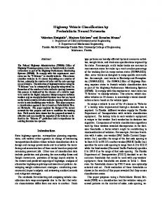
Fig. 1. Component parameters θmn in chess-board arrangement corresponding to the typical variants of samples (|Mω | = 50). The parameters θnm are displayed by greylevels inversely (0 = white, 1 = black). The different ”style” of patterns of both classes is well apparent.

the mixture model, (|Mω | = 1, 2, 5, 10, 20, 50, 100, 200, 500) and the size of the training set (|Sω | = 103 , 104 , 105 ). For the sake of independent testing we have used one pair of sufficiently large sets (2 × 105 patterns for each class). Obviously this approach is not very realistic since in practical situation a large test set is usually not available. However, in this way the test set performance in our experiments is verified with a high level of reliability and we avoid an additional source of noise. In all computations the initial mixture parameters θnm have been chosen randomly with the uniform weights f (m) = 1/|Mω |. Certainly, there is some random influence of the starting point (especially in case of the small sample size) but in repeated computations with different starting points we have obtained comparable results. The EM-iterations have been stopped

38

J. Grim and J. Hora

Table 1. Results of numerical experiments with full multivariate Bernoulli mixtures M K 1 000 2 512 34.70 % 4 1024 13.10 % 10 2560 1.65 % 20 5120 0.95 % 40 10240 0.15 % 100 25600 0.00 % 200 51200 0.00 % 400 102400 0.00 % 1000 256000 0.00 %

200 000 41.56 % 15.83 % 7.72 % 9.21 % 8.76 % 9.35 % 11.02 % 15.40 % 17.77 %

10 000 39.59 % 16.54 % 6.60 % 5.40 % 3.91 % 2.01 % 1.22 % 0.69 % 0.20 %

200 000 40.38 % 16.65 % 7.00 % 5.90 % 4.90 % 4.54 % 5.57 % 8.35 % 14.66 %

100 000 39.90 % 16.42 % 6.49 % 4.04 % 2.73 % 1.37 % 0.84 % 0.45 % 0.14 %

200 000 40.02 % 16.48 % 6.60 % 4.34 % 2.89 % 1.90 % 1.68 % 1.92 % 3.76 %

when the relative increment of the likelihood function (Q − Q)/Q was less then 0.0001. In all experiments the convergence of EM algorithm has been achieved in less than 40 iterations. The resulting estimates of the conditional distributions P (x|ω1 ), P (x|ω2 ) have been used to perform the Bayesian classification both of the training- and independent test patterns according to maximum a posteriori probability (cf. (1), (15)). Figure 1 graphically displays the parameters of the estimated full mixture components (|Mω | = 50) both for the class “knight” and “rook”. The parameters θnm are arranged to correspond to the underlying chess board, the parameter values are displayed by grey-levels inversely (0 = white, 1 = black). Note that the style of the component patterns suggests the nature of random moves.

4

Example - Full Mixture Model

In the first part of the numerical experiment we have used full mixture model including 256 parameters for each component. We estimated the class-conditional mixtures for the number of components increasing from M=1 to M=500 in each class. The total number of components (2M) for the respective solution is given in the first column of Table 1, the second column contains the corresponding total number of parameters increasing form K=512 to a relatively high value K=256000. For simplicity, we do not count component weights as parameters. The class-conditional mixtures have been estimated for three differently large training sets (|Sω | = 103 , 104 , 105 ). The corresponding recognition error computed on the training set is given in the columns 3, 5 and 7 respectively, the corresponding error estimated on the independent test set (|Sω | = 2 × 105 ) is given in the columns 4,6 and 8 respectively. It can be seen that even small training data set (|Sω | = 103 ) is sufficient to estimate the underlying 256 parameters reasonably. The classification error on the test set is about 40% and it is comparable with the respective training-set error. Thus, in the second row, the effect of overfitting is rather small because of the underlying model simplicity. In the last row the complex mixtures of 500 components (1000 totally) strongly overfit by showing the training set error near zero. The related independent test set


39

Table 2. Results of numerical experiments with the structural mixture model M K 1 000 4 830 13.80 % 8 1650 6.45 % 20 3770 5.70 % 40 7010 8.65 % 80 13500 4.20 % 200 32700 0.25 % 400 65000 0.00 % 800 128100 0.00 % 2000 317200 0.00 %

200 000 16.48 % 9.97 % 10.97 % 13.63 % 12.91 % 11.46 % 18.11 % 18.50 % 18.75 %

10 000 25.53 % 10.96 % 5.14 % 4.20 % 6.12 % 3.36 % 3.54 % 3.88 % 2.84 %

200 000 26.53 % 11.32 % 5.77 % 4.73 % 6.88 % 4.76 % 4.70 % 4.82 % 6.39 %

100 000 16.91 % 7.28 % 4.70 % 3.29 % 1.91 % 1.83 % 3.10 % 5.42 % 2.71 %

200 000 16.92 % 7.29 % 4.72 % 3.32 % 1.92 % 1.85 % 3.20 % 5.45 % 2.73 %

error (|Sω | = 2 × 105) decreases from about 17.77% to 3.76% in the last column. Obviously the class-conditional mixtures including 128 thousand of parameters need more data to be reasonably estimated, otherwise the effect of overfitting is rather strong. Because of overfitting the recognition of training patterns is generally more accurate than that of independent test patterns. Expectedly, the training-set error decreases with the increasing complexity of class conditional mixtures because of increasingly tight adaptation to training data. However, because of overfitting, the training-set error would be a wrong criterion to choose model complexity. It can be seen that, in Table 1, the optimal number of components is different for different size of training set. In view of the independent test-set error we should use 5 components for each class-conditional mixture in case of training set |Sω | = 103 , (M=10, row 4), 50 components for the training set |Sω | = 104 , (M=100, row 7) and 100 components for |Sω | = 105 , (M=200, row 8).

5

Example - Structural Mixture Model

In the second part of the numerical experiments we recomputed the results of Table 1 by means of structural mixture model. By using a low threshold coefficient C0 = 0.1 (cf. Eq. (16)) we exclude only parameters which are nearly superfluous in evaluation of mixture components. In order to compensate for the omitted parameters we have used twice more mixture components. In this way we have obtained a similar model complexity in the second column of Table 2. At the first view the recognition accuracy in the second row is much better than in the Table 1. The differences illustrate the trivial advantage of the twocomponent mixtures in comparison with the single product components in Table 1. Expectedly, the structural mixture model is much less overfitting and therefore the differences between the respective training-set- and test-set errors are smaller (possibly except for the small training set |Sω | = 103 , column 3 and 4). In case of the two large training sets (|Sω | = 104 , 105 ) the overfitting effect is almost negligible. In the last rows the training set errors are greater than in Table 1 because the information criterion (14) reduces the fitting of components to

40

J. Grim and J. Hora

highly specific types of patterns. As it can be seen, the training-set error could be used to select the structural model complexity almost optimally. Thus we would choose M=200 components both for the training sets |Sω | = 104 and 105 .

6

Concluding Remark

The complex multivariate Bernoulli mixtures with many components tend to overfit mainly by fitting the components to highly specific types of patterns or even to outliers. We assume that the ”less informative” parameters are responsible for overfitting of the ”full” multivariate Bernoulli mixture in Table 1. This mechanism of overfitting may be reduced by using structural mixture model since the fitting of components to outliers is disabled by means of informativity threshold. As it can be seen in Table 2 the resulting training set error of structural mixtures would enable almost correct choice of the model complexity. ˇ No. 102/07/1594 of Czech Acknowledgement. Supported by the project GACR ˇ Grant Agency and by the projects 2C06019 ZIMOLEZ and MSMT 1M0572 DAR.

References 1. Dempster, A.P., Laird, N.M., Rubin, D.B.: Maximum likelihood from incomplete data via the EM algorithm. J. of the Royal Stat. Soc. B 39, 1–38 (1977) 2. Dietterich, T.: Overfitting and undercomputing in machine learning. ACM Computing Surveys 27(3), 326–327 (1995) 3. Grim, J.: Multivariate statistical pattern recognition with nonreduced dimensionality. Kybernetika 22, 142–157 (1986) 4. Grim, J.: Information approach to structural optimization of probabilistic neural networks. In: Ferrer, L., et al. (eds.) Proceedings of 4th System Science European Congress, pp. 527–540. Soc. Espanola de Sistemas Generales, Valencia (1999) 5. Grim, J., Just, P., Pudil, P.: Strictly modular probabilistic neural networks for pattern recognition. Neural Network World 13, 599–615 (2003) 6. Grim, J.: Neuromorphic features of probabilistic neural networks. Kybernetika 43(6), 697–712 (2007) 7. Grim, J., Hora, J.: Iterative principles of recognition in probabilistic neural networks. Neural Networks 21(6), 838–846 (2008) 8. McLachlan, G.J., Peel, D.: Finite Mixture Models. John Wiley and Sons, New York (2000) 9. Sarle, W.S.: Stopped training and other remedies for overfitting. In: Proceedings of the 27th Symposium on the Interface (1995), ftp://ftp.sas.com/pub/neural/inter95.ps.Z 10. Schaffer, C.: Overfitting avoidance as Bias. Machine Learning 10(2), 153–178 (1993) 11. Schlesinger, M.I.: Relation between learning and self-learning in pattern recognition. Kibernetika (Kiev) (2), 81–88 (1968) (in Russian) 12. Specht, D.F.: Probabilistic neural networks for classification, mapping or associative memory. In: Proc. IEEE Int. Conf. on Neural Networks, vol. I, pp. 525–532 (1988) 13. Vajda, I.: Theory of Statistical Inference and Information. Kluwer, Boston (1992) 14. Yinyin, L., Starzyk, J.A., Zhu, Z.: Optimized Approximation Algorithm in Neural Networks Without Overfitting. IEEE Tran. Neural Networks 19, 983–995 (2008)