Computational Visual Attention Simone Frintrop
Visual attention is one of the key mechanisms of perception that enables humans to efficiently select the visual data of most potential interest. Machines face similar challenges as humans: they have to deal with a large amount of input data and have to select the most promising parts. In this chapter, we explain the underlying biological and psychophysical grounding of visual attention, show how these mechanisms can be implemented computationally, and discuss why and under what conditions machines, especially robots, profit from such a concept.
1 What Is Attention? And Do We Need Attentive Machines? Attention is one of the key mechanisms of human perception that enables us to act efficiently in a complex world. Imagine you visit Cologne for the first time, you stroll through the streets and look around curiously. You look at the large Cologne Cathedral and at some street performers. After a while, you remember that you have to catch your train back home soon and you start actively to look for signs to the station. You have no eye for the street performers any more. But when you enter the station, you hear a fire alarm and see that people are running out of the station. Immediately you forget your waiting train and join them on their way out. This scenario shows the complexity of human perception. Plenty of information is perceived at each instant, much more than can be processed in detail by the human brain. The ability to extract the relevant pieces of the sensory input at an early processing stage is crucial for efficient acting. Thereby, it depends on the context which part of the sensory input is relevant. When having a goal like catching a train, the signs are relevant, without an explicit goal, salient things like the street performers attract the attention. Some things or events are so salient that they even override Simone Frintrop Rheinische Friedrich-Wilhelms Universit¨at Bonn, Institute of Computer Science III, R¨omerstrasse 164, 53117 Bonn; e-mail:
[email protected]
1
2
Simone Frintrop
your goals, such as the fire alarm. The mechanism to direct the processing resources to the potentially most relevant part of the sensory input is called selective attention. One of the most famous definitions of selective attention is from William James, a pioneering psychologist, who stated in 1890: “Everyone knows what attention is. It is the taking possession by the mind, in clear and vivid form, of one out of what seem several simultaneously possible objects or trains of thought” [11]. While the concept of attention exists for all senses, here we will concentrate on visual attention and thus on the processing of images and videos. While it is obvious that attention is a useful concept for humans, why is it of interest for machines and which kinds of machines profit most from such a concept? To answer these questions, let us tackle two goals of attention separately. The first goal is to handle the complexity of the perceptual input. Since many visual processing tasks concerned with the recognition of arbitrary objects are NP-hard [23], an efficient solution is often not achievable. Problems arise for example if arbitrary objects of arbitrary sizes and extends shall be recognized, i.e. everything from the fly on the wall to the building in the background. The typical approach to detect objects in images is the sliding-window paradigm in which a classifier is trained to detect an object in a subregion of the image and is repeatedly applied to differently sized test windows. A mechanism to prioritize the image regions for further processing is of large interest, especially if large image databases shall be investigated or if real-time processing is desired, e.g. on autonomous mobile robots. The second goal of attention is to support action decisions. This task is especially important for autonomous robots that act in a complex, possibly unknown environment. Even if equipped with unlimited computational power, robots still underlie similar physical constraints as humans: at one point in time, they can only navigate to one location, zoom in on one or a few regions, and grasp one or a few objects. Thus, a mechanism that selects the relevant parts of the sensory input and decides what to do next is essential. Since robots usually operate in the same environments as humans, it is reasonable to imitate the human attention system to fulfill these tasks. Furthermore, in domains as human-robot interaction, it is helpful to generate a joint focus of attention between man and machine to make sure that both communicate about the same object1 . Having similar mechanisms for both human and robot facilitates this task. As a conclusion, we can state that the more general a system shall be and the more complex and undefined the input data are, the more urgent the need for a prioritizing attention system that preselects the data of most potential interest. This chapter aims to provide you with everything you must know to build a computational attention system2 . It starts with an introduction to human perception (sec. 2). This section gives you an insight to the important mechanisms in the brain that are involved in visual attention and thus provides the background knowledge that is required when working in the field of computational attention. If you are mainly interested in how to build a computational system, you might skip this 1 2
The social aspect of human attention is described in chapter 8, section 5.4.1 Parts of this chapter have been published before in [4].
Computational Visual Attention
3
Fig. 1 Left: The human visual system (Fig. adapted from http://www.brain-maps.com/visualfields.html). Right: The receptive field of a ganglion cell with center and surround and its simulation with Difference-of-Gaussian filters (Fig. adapted from [15]).
section and directly jump to sec. 3. This section explains how to build a bottomup system of visual attention and how to extend such a system to perform visual search for objects. After that, we discuss different ways to evaluate attention systems (sec. 4) and mention two applications of such systems in robotic contexts (sec. 5). At the end of the chapter you find some useful links to Open Source code, freely accessible databases, and further readings on the topic.
2 Human Visual Attention In this section, we will introduce some of the cognitive foundations of human visual attention. We start with the involved brain mechanisms, continue with several psychological concepts and evaluation methods, and finally present two influential psychological models.
2.1 The Human Visual System Let us first regard some of the basic concepts of the human visual system. While being far from an exhaustive explanation, we focus on describing parts that are necessary to understand the visual processing involved in selective attention. The most important visual areas are illustrated in Fig. 1, left.
2.1.1 Eye, Retina, and Ganglion Cells The light that enters the eye through the pupil passes through the lens, and reaches the retina at the back of the eye. The retina is a light-sensitive surface and is densely covered with over 100 million photoreceptor cells, rods and cones. The rods are more numerous and more sensitive to light than the cones but they are not sensitive
4
Simone Frintrop
to color. The cones provide the eye’s color sensitivity: among the cones, there are three different types of color reception: long-wavelength cones (L-cones) which are sensitive primarily to the red portion of the visible spectrum, middle-wavelength cones (M-cones) sensitive to green, and short-wavelength cones (S-cones) sensitive to blue. In the center of the retina is the fovea, a rod-free area with very thin, densely packed cones. It is the center of the eye’s sharpest vision. Because of this arrangement of cells, we perceive the small region currently fixated in a high resolution and the whole surrounding only diffuse and coarse. This mechanism makes eye movements an essential part of perception, since they enable high resolution vision subsequently for different regions of a scene. The photoreceptors transmit information to the so called ganglion cells, which combine the trichromatic input by subtraction and addition to determine color and luminance opponency. The receptive field of a ganglion cell, i.e. the region the cell obtains input from, is circular and separated into two areas: a center and a surround (cf. Fig. 1, right). There are two types of cells: on-center cells which are stimulated by light at the center and inhibited by light at the surround, and off-center cells with the opposite characteristic. Thus, on-center cells are well suited to detect bright regions on a dark background and off-center cells vice versa. Additional to the luminance contrast, there are also cells that are sensitive to red-green and to blue-yellow contrasts. The center-surround concept of visual cells can be modeled computationally with Difference-of-Gaussian filters (cf. Fig. 1, right) and is the basic mechanism for contrast detection in computational attention systems.
2.1.2 From the Optic Chiasm to V1 The visual information leaves the eye via the optic nerve and runs to the optic chiasm. From here, two pathways go to each brain hemisphere: the smaller one goes to the superior colliculus (SC), which is e.g. involved in the control of eye movements. The more important pathway goes to the Lateral Geniculate Nucleus (LGN) and from there to higher brain areas. The LGN consists of six main layers composed of cells that have center-surround receptive fields similar to those of retinal ganglion cells but larger and with a stronger surround. From the LGN, the visual information is transmitted to the primary visual cortex (V1) at the back of the brain. V1 is the largest and among the best-investigated cortical areas in primates. It has the same spatial layout as the retina itself. But although spatial relationships are preserved, the densest part of the retina, the fovea, takes up a much smaller percentage of the visual field (1%) than its representation in the primary visual cortex (25%). The cells in V1 can be classified into three types: simple cells, complex cells, and hypercomplex cells. As the ganglion cells, the simple cells have an excitatory and an inhibitory region. Most of the simple cells have an elongated structure and, therefore, are orientation sensitive. Complex cells take input from many simple cells. They have larger receptive fields than the simple cells and some are sensitive to moving lines or edges. Hypercomplex cells, in turn, receive the signals from com-
Computational Visual Attention
5
plex cells as input. These neurons are capable of detecting lines of a certain length or lines that end in a particular area.
2.1.3 Beyond V1: the Extrastriate Cortex and the Visual Pathways From the primary visual cortex, a large collection of neurons sends information to higher brain areas. These areas are collectively called extrastriate cortex, in opposite to the striped architecture of V1. The areas belonging to the extrastriate cortex are V2, V3, V4, the infero-temporal cortex (IT), the middle temporal area (MT or V5) and the posterior-parietal cortex (PP).3 On the extrastriate areas, much less is known than on V1. One of the most important findings of the last decades was that the processing of the visual information is not serial but highly parallel. While not completely segregated, each area has a prevalence of processing certain features such as color, form (shape), or motion. Several pathways lead to different areas in the extrastriate cortex. The statements on the number of existing pathways differ: the most common belief is that there are three main pathways, one color, one form, and one motion pathway which is also responsible for depth processing [12]. The color and form pathways go through V1, V2, and V4 and end finally in IT, the area where the recognition of objects takes place. In other words, IT is concerned with the question of “what” is in a scene. Therefore, the color and form pathway together are called the what pathway. It is also called ventral stream because of its location on the ventral part of the body. The motion-depth pathway goes through V1, V2, V3, MT, and the parieto occipale area (PO) and ends finally in PP, responsible for the processing of motion and depth. Since this area is mainly concerned with the question of “where” something is in a scene, this pathway is also called where pathway. Another name is dorsal stream because it is considered to lie dorsally. Finally, it is worth to mention that although the processing of the visual information was described above in a feed-forward manner, it is usually bi-directional. Topdown connections from higher brain areas influence the processing and go down as far as LGN. Also lateral connections combine the different areas, for example, there are connections between V4 and MT, showing that the “what” and “where” pathway are not completely separated.
2.1.4 Neurobiological Correlates of Visual Attention The mechanisms of selective attention in the human brain still belong to the open problems in the field of research on perception. Perhaps the most prominent outcome of neuro-physiological findings on visual attention is that there is no single brain area guiding the attention, but neural correlates of visual selection appear to be reflected in nearly all brain areas associated with visual processing. Attentional 3
The notation V1 to V5 comes from the former belief that the visual processing would be serial.
6
Simone Frintrop
mechanisms are carried out by a network of anatomical areas. Important areas of this network are the posterior parietal cortex (PP), the superior colliculus (SC), the Lateral IntraParietal area (LIP), the Frontal Eye Field (FEF) and the pulvinar. Brain areas involved in guiding eye movements are the FEF and the SC. There is also evidence that a kind of saliency map exists in the brain, but the opinions where it is located diverge. Some researchers locate it in the FEF, others at the LIP, the SC, at V1 or V4 (see [4] for references). Further research will be necessary to determine the tasks and interplay of the brain areas involved in the process of visual attention.
2.2 Psychological Concepts of Attention Certain concepts and expressions are frequently used when investigating human visual attention and shall be introduced here. Usually, directing the focus of attention to a region of interest is associated with eye movements (overt attention). However, it is also possible to attend to peripheral locations of interest without moving the eyes, a phenomenon which is called covert attention. The allocation of attention is guided by two principles: bottom-up and top-down factors. Bottom-up attention (or saliency) is derived solely from the perceptual data. Main indicators for visual bottom-up saliency are a strong contrast of a region to its surround and the uniqueness of this region. Thus, a clown in the parliament is salient, whereas it is not particularly salient among other clowns (however, a whole group of clowns in the parliament is certainly salient!). The bottom-up influence is not voluntary suppressible: a highly salient region captures your attention regardless of the task, an effect called attentional capture. This effect might save your life, e.g. if an emergency bell or a fire captures your attention. On the other hand, top-down attention is driven by cognitive factors such as preknowledge, context, expectations, and current goals. In human viewing behaviour, top-down cues always play a major role. Not only looking for the train station signs in the introductory example is an example of top-down attention, also more subtle influences like looking at food when being hungry. In psychophysics, top-down influences are often investigated by so called cueing experiments, in which a cue directs the attention to a target. A cue might be an arrow that points into the direction of the target, a picture of the target, or a sentence (“search for the red circle”). One of the best investigated aspect of top-down attention is visual search. The task is exactly what the name implies: given a target and an image, find an instance of the target in the image. Visual search is omnipresent in every-day life: finding a friend in a crowd or your keys in the livingroom are examples. In psychophysical experiments, the efficiency of visual search is measured by the reaction time (RT) that a subject needs to detect a target among a certain number of distractors (the elements that differ from the target) or by the search accuracy. To measure the RT, a subject has to report a detail of the target or has to press one button if the target was detected and another if it is not present in the scene. The RT is represented as a function of set size (the number of elements in the display).
Computational Visual Attention
(a) Feature search
7
(b) Conjunction search
(c) Continuum of search slopes
Fig. 2 (a) Feature search: the target (horizontal line) differs from the distractors (vertical lines) by a unique visual feature (pop-out effect). (b) Conjunction search: the target (red, horizontal line) differs from the distractors (red, vertical and black, horizontal lines) by a conjunction of features. (c) The reaction time (RT) of a visual search task is a function of set size. The efficiency is measured by the intercept and slopes of the functions (Fig. redrawn from [27]).
The search efficiency is determined by the slopes and the intercepts of these RT × set size functions (cf. Fig. 2 (c)). The searches vary in their efficiency: the smaller the slope of the function and the lower the value on the y-axis, the more efficient the search. Two extremes are serial and parallel search. In serial search, the reaction time increases with the number of distractors, whereas in parallel search, the slope is near zero. But note that the space of search slope functions is a continuum. Feature searches take place in settings in which the target is distinguished from the distractors by a single basic feature (such as color or orientation)(cf. Fig. 2, (a)). In conjunction searches on the other hand, the target differs by more than one feature (see Fig. 2 (b)). While feature searches are usually fast and conjunction searches slower, this is not generally the case. Also a feature search might be slow if the difference between target and distractors is small (e.g. a small deviation in orientation). Generally, it can be said that search becomes harder as the target-distractor similarity increases and easier as distractor-distractor similarity increases. The most efficient search takes place for so called “pop-out” experiments that denote settings in which a single element immediately captures the attention of the observer. You understand easily what this means by looking at Fig. 2 (a). Other methods to investigate visual search is by measuring accuracy or eye movements. References for further readings on this topic can be found in [6]. One purpose of such experiments is to study the basic features of human perception, that means the features that are early and pre-attentively processed in the human brain and guide visual search. Undoubted basic features are color, motion, orientation and size (including length and spatial frequency) [28]. Some other features are guessed to be basic but there is limited data or dissenting opinions. An interesting effect in visual search tasks are search asymmetries, that means the effect that a search for stimulus ’A’ among distractors ’B’ produces different results than a search for ’B’ among ’A’s. An example is that finding a tilted line among vertical distractors is easier than vice versa. An explanation is proposed by [22]: the authors claim that it is easier to find deviations among canonical stimuli than vice versa. Given that vertical is a canonical stimulus, the tilted line is a deviation and may be detected quickly.
8
Simone Frintrop
(a) Feature integration theory
(b) Guided search model
Fig. 3 Left: Model of the Feature Integration Theory (FIT) (Fig. redrawn from [20]) Right: The c Guided Search model of Wolfe (Fig. adapted from [26] ⃝1994 Psychonomic Society).
2.3 Important Psychological Attention Models In the field of psychology, there exists a wide variety of theories and models on visual attention. Their objective is to explain and better understand human perception. Here, we introduce two approaches which have been most influential for computational attention systems. The Feature Integration Theory (FIT) of Treisman claims that “different features are registered early, automatically and in parallel across the visual field, while objects are identified separately and only at a later stage, which requires focused attention” [21]. Information from the resulting feature maps — topographical maps that highlight conspicuities according to the respective feature — is collected in a master map of location. Scanning serially through this map focuses the attention on the selected scene regions and provides this data for higher perception tasks (cf. Fig. 3 (a)). The theory was first introduced in 1980 but it was steadily modified and adapted to current research findings. Beside FIT, the Guided Search Model of Wolfe is among the most influential work for computational visual attention systems [26]. The basic goal of the model is to explain and predict the results of visual search experiments. Mimicking the convention of numbered software upgrades, Wolfe has denoted successive versions of his model as Guided Search 1.0 to Guided Search 4.0. The best elaborated description of the model is available for Guided Search 2.0 [26]. The architecture of the model is depicted in Figure 3 (b). It shares many concepts with the FIT, but is more detailed in several aspects which are necessary for computer implementations. An interesting point is that in addition to bottom-up saliency, the model also considers the influence of top-down information by selecting the feature type which distinguishes the target best from its distractors.
Computational Visual Attention
9
3 Computational Attention Systems Computational attention systems model the principles of human selective attention and aim to select the part of the sensory input data that is most promising for further investigation. Here, we concentrate on visual attention systems that are inspired by concepts of the human visual system but are designed with an engineering objective, that means their purpose is to improve vision systems in technical applications.4
3.1 General structure Most computational attention systems have a similar structure, which is depicted in Fig. 4. This structure is originally adapted from psychological theories like the Feature Integration Theory and the Guided Search model (cf. Sec. 2.3). The main idea is to compute several features in parallel and to fuse their conspicuities in a saliency map. If top-down information is available, this can be used to influence the processing at various levels of the models. A saliency map is usually a gray-level image in which the brightness of a pixel is proportional to its saliency. The maxima in the saliency map denote the regions that are investigated by the focus of attention (FOA) in the order of decreasing saliency. This trajectory of FOAs shall resemble human eye movements. Output of a computational attention system is either the saliency map or a trajectory of focused regions. While most attention systems share this general structure, there are different ways to implement the details. One of the best known computational attention systems is the iNVT from Itti and colleagues [10]. The VOCUS model [4] has adopted and extended several of their ideas. It is real-time capable and has a top-down mode to search for objects (visual search). Itti and Baldi presented an approach that is able to detect temporally salient regions, called surprise theory [8]. Bruce and Tsotsos compute saliency by determining the self-information of image regions with respect to their surround [1]. The types of top-down information that can influence an attention model are numerous and only a few have been realized in computational system. For example, the VOCUS model uses pre-knowledge about a target to weight the feature maps and perform visual search. Torralba et al. use context information about the scene to guide the gaze, e.g., to search for people on the street level of an image rather than on the sky area [19]. More abstract types of top-down cues, such as emotions and motivations, have to our knowledge not yet been integrated into computational attention systems. In this chapter, we follow the description of the VOCUS model as representative of one of the classic approaches to compute saliency.5 We start with introducing the 4
In this chapter, we assume that the reader has basic knowledge on image processing, otherwise you find a short explanation of the basic concepts in the appendix of [4]. 5 While the description here is essentially the same as in [4], some improvements have been made in the meantime that are included here. Differences of VOCUS to the iNVT can be found in [4].
10
Simone Frintrop
Fig. 4 General structure of most visual attention systems. Several features are computed in parallel and fused to a single saliency map. The maxima in the saliency map are the foci of attention (FOAs). Output is a trajectory of FOAs, ordered by decreasing saliency. Top-down cues may influence the processing on different levels.
bottom-up part (Sec. 3.2), followed by a description of the top-down visual search part (Sec. 3.3).
3.2 Bottom-up saliency Bottom-up saliency is usually a combination from different feature channels. The most frequently used features in visual attention systems are intensity, color, and orientation. When image sequences are processed, also motion and flicker are important. The main concept to compute saliency are contrast computations that determine the difference between a center region and a surrounding region with respect to a certain feature. These contrasts are usually computed by center-surround filters. Such filters are inspired by cells in the human visual system, as the ganglion cells and the simple and complex cells introduced in Sec. 2.1. Cells with circular receptive fields are best modeled by Difference-of-Gaussian filters (cf. Fig. 1, right) while cells with elongated receptive fields are best modeled by Gabor functions. In practice, the circular regions are usually approximated by rectangles. To enable the detection of regions of different extends, the center as well as the surround vary in size. Instead of directly adapting the filter sizes, the computations are usually performed on the layers of an image pyramid. The structure of the bottom-up part of the attention system VOCUS is shown in Fig. 5. Let us regard the computation of the intensity feature in more detail now to understand the concept and then extend the ideas to the other feature channels.
3.2.1 Intensity Channel Given a color input image I, this image is first converted to an image ILab in the Lab (or CIELAB) color space. This space has the dimension ’L’ for lightness and ’a’ and ’b’ for the color-opponent dimensions (cf. Fig. 5, bottom right); it is perceptually
Computational Visual Attention
Fig. 5 The bottom-up saliency computation of the attention system VOCUS.
11
12
Simone Frintrop
(a) Input image
(b) Gaussian pyramid, s0 to s4
Fig. 6 The image which serves as demonstration example throughout this chapter (a) and the derived Gaussian image pyramid (b).
uniform, which means that a change of a certain amount in a color value is perceived as a change of about the same amount in human visual perception. From ILab , a Gaussian pyramid is determined by successively smoothing the image with a Gaussian filter and subsampling it with a factor of 2 along each coordinate direction (see Fig. 6). In VOCUS, we use a 5 × 5 Gaussian kernel. The level of the pyramid determines the area that the center-surround filter covers: on high levels of the pyramid (fine resolution), small salient regions are detected while on low levels (coarse resolution), large regions obtain the highest response. In VOCUS, 5 pyramid s , s ∈ {0, .., 4}. Level I 1 is only an intermediate levels (scales) are computed: ILab Lab step used for noise reduction, all computations take place on levels 2 – 4.6 The intensity computations can be performed directly on the images ILs that originate from the ’L’ channel of the LAB image. According to the human system, we determine two feature types for intensity: the on-center difference responding strongly to bright regions on a dark background, and the off-center difference vice versa. Note that it is important to treat both types separately and to not fuse them in a single map since otherwise it is not possible to detect bright′′ dark pop-outs, such as in Fig. 12. This yields 12 intensity scale maps Ii,s, σ with i ∈ {(on), (off)}, s ∈ {2, 3, 4}, σ ∈ {3, 7}. A pixel (x,y) in one of the on-center scale maps is thus computed as: ′′ s s Ion,s, σ (x, y) = center(IL , x, y) − surroundσ (IL , x, y) ( ) σ σ 1 s s s = IL (x, y) − ∑ ∑ IL (x + i, y + j) − IL (x, y) (2 σ + 1)2 − 1 i=− σ j=−σ
(1) ′′ The off-center maps Ioff ,s,σ (x, y) are computed equivalently by surround − center. The straight-forward computation of the surround value is quite costly, especially for large surrounds. To compute the surround value efficiently, it is convenient to use integral images [24]. 6
The number of levels that is reasonable depends on the image size as well as on the size of the objects you want to detect. Larger images and a wide variety of possible object sizes require deeper pyramids. The presented approach usually works well for images of up to 400 pixels in width and height in which the objects are comparatively small as in the example images of this chapter.
Computational Visual Attention
13
Fig. 7 Left: The integral image contains at II(x, y) the sum of the pixel values in the shaded region. Right: the computation of the average value in the shaded region is based on four operations on the four depicted rectangles according to eq. 5.
The advantage of an integral image (or summed area table) is that when it is once created, the sum and mean of the pixel values of a rectangle of arbitrary size can be computed in constant time. An integral image II is an intermediate representation for the image and contains for a pixel position (x,y) the sum of all gray scale pixel values of image I above and left of (x,y), inclusive: x
II(x, y) =
y
I(x′ , y′ ). ∑ ∑ ′ ′
(2)
x =0 y =0
The process is visualized in Fig. 7, left. The integral image can be computed recursively in one pass over the image with help of the cumulative sum s: s(x, y) = s(x, y − 1) + I(x, y) II(x, y) = II(x − 1, y) + s(x, y)
(3) (4)
with s(x, −1) = 0 and II(−1, y) = 0. This intermediate representation allows to compute the sum of the pixel values in a rectangle F using four references (see Fig. 7 (right)): F(x, y, h, w) = II(x + w − 1, y + h − 1) − II(x − 1, y + h − 1) −II(x + w − 1, y − 1) + II(x − 1, y − 1).
(5)
The ’-1’ elements in the equation are required to obtain a rectangle that includes (x,y). By replacing the computation of the surround in (1) with the integral computation in (5) we obtain: ′′ s Ion,s, σ (x, y) = IL (x, y) −
F(x − σ , y − σ , 2σ + 1, 2σ + 1) − ILs (x, y) (2 σ + 1)2 − 1
(6)
14
Simone Frintrop
′′ . First row: the on-maps. Second row: the off-maps. Fig. 8 Left: the 12 intensity scale maps Ii,s, σ ′ ′ Right: the two intensity feature maps I(on) and I(off) resulting from the sum of the corresponding six scale maps on the left.
To enable this computation, one integral image has to be computed for each of the three pyramid levels ILs , s ∈ {2, 3, 4}. This pays off since then each surround can be determined by three simple operations. The intensity scale maps I ′′ are depicted in Fig. 8, left. The six maps for each center-surround variation are summed up by across-scale addition: first, all maps are resized to scale 2 whereby resizing scale i to scale i − 1 is done by bilinear interpolation. After resizing, the maps are added up pixel by pixel. This yields the intensity feature maps I ′ : Ii′ =
⊕ s,σ
′′ Ii,s, σ,
(7) ⊕
with i ∈ {(on), (off)}, s ∈ {2, 3, 4}, σ ∈ {3, 7}, and denoting the across-scale addition. The two intensity feature maps are shown in Fig. 8, right.
3.2.2 Color Channel The color computations are performed on the two-dimensional color layer Iab of the Lab image that is spanned by the axes ’a’ and ’b’. Besides its resemblance to human visual perception, the Lab color space fits particularly well as basis for an attentional color channel since the four main colors red, green, blue and yellow are at the end of the axes ’a’ and ’b’. Each of the 6 ends of the axes that confine the color space serves as one prototype color, resulting in two intensity prototypes for white and black and four color prototypes for red, green, blue, and yellow. For each color prototype, a color prototype image is computed on each of the pyramid levels 2 – 4. In these maps, each pixel represents the Euclidean distance to the prototype: s Cγs (x, y) = Vmax − ||Iab (x, y) − Pγ ||,
γ ∈ {R,G,B,Y},
(8)
Computational Visual Attention
15
Fig. 9 Top: the color prototype images of scale s2 for red, green, blue, yellow. Bottom: the corresponding color feature Cγ′ maps which result after applying center-surround filters.
where Vmax is the maximal pixel value and the prototypes Pγ are the ends of the ’a’ and ’b’ axes (thus, in an 8-bit image, we have Vmax = 255 and PR = (255, 127), PG = (0, 127), PB = (127, 0), PY = (127, 255)). The color prototype maps show to which degree a color is represented in an image, i.e., the maps in the pyramid PR show the “redness” of the image regions: the brightest values are at red regions and the darkest values at green regions (since green has the largest distance to red in the color space). Analogical to the intensity channel, it is also important here to separate red-green and blue-yellow in different maps to enable red-green and blue-yellow pop-outs. The four color prototype images Iγ2 are displayed in Fig. 9, top. On these pyramids, the color contrast is computed by on-center differences yielding 4 ∗ 3 ∗ 2 = 24 color scale maps: Cγ′′,s,σ = center(Cγs , x, y) − surroundσ (Cγs , x, y),
(9)
with γ ∈ {R,G,B,Y}, s ∈ {2, 3, 4}, and σ ∈ {3, 7}. According to the intensity channel, the center is a pixel in the corresponding color prototype map, and the surround is computed according to eq. 6. The off-center-on-surround difference is not needed, because these values are represented in the opponent color pyramid. The maps of each color are rescaled to the scale 2 and summed up into 4 color feature maps Cγ′ : Cγ′ =
⊕ s,σ
Cγ′′,s,σ .
(10)
Fig. 9, bottom shows the color feature maps for the example image.
3.2.3 Orientation Channel The orientation maps are computed from oriented pyramids. An oriented pyramid contains one pyramid for each represented orientation (cf. Fig.10, left). Each of these pyramids highlights edges with this specific orientation. To obtain the oriented pyramid, first a Laplacian Pyramid is obtained from the Gaussian pyramid ILs by subtracting adjacent levels of the pyramid. The orientations are computed by Gabor filters which respond most to bar-like features according to a specified orien-
16
Simone Frintrop
Fig. 10 Left: to obtain an oriented pyramid, a Gaussian pyramid is computed from the input image, then a Laplacian pyramid is obtained from the Gaussian pyramid by subtracting two adjacent levels and, finally, Gabor filters of 4 orientations are applied to each level of the Laplacian pyramid. Right: The four orientation feature maps O′0 ◦ , O′45 ◦ , O′90 ◦ , O′135 ◦ for the example image.
tation. Gabor filters, which are the product of a symmetric Gaussian with an oriented sinusoid, simulate the receptive field structure of orientation-selective cells in the primary visual cortex (cf. 2.1). Thus, the Gabor filters replace the center-surround filters of the other channels. Four different orientations are computed yielding 4 × 3 = 12 orientation scale maps O′′θ ,s , with the orientations θ ∈ {0 ◦ , 45 ◦ , 90 ◦ , 135 ◦ } and scales s ∈ {2, 3, 4}. The orientation scale maps O′′θ ,s are summed up by across-scale addition for each orientation, yielding four orientation feature maps O′θ , one for each orientation: Oθ′ =
⊕
O′′θ ,s ,
(11)
s
The orientation feature maps for the example image are depicted in Fig. 10, right.
3.2.4 Motion Channel If image sequences are used as input for the attention system, motion is an important additional feature. It can be computed easily by determining the optical flow field. Here, we use a method based on total variation regularization that determines a dense optical flow field and is capable to operate in real-time [29]. If the horizontal u and the vertical v component of the optical flow are visualized as images, the center-surround filters can be applied to these images directly. By applying on- as well as off-center filters to both images, we achieve four motion maps for each scale s which we call Mϑ′′ ,s , with ϑ = {right, left, up, down}. After accross-scale addition we obtain four motion feature maps
Computational Visual Attention
17
Fig. 11 The motion feature maps M ′ for a scene in which a ball rolls from right to left through the ′ ′ , M′ , M′ image. From left to right: example frame, motion maps Mright , Mleft up down .
Mϑ′ =
⊕
Mϑ′′ ,s .
(12)
s
An example for a sequence in which a ball rolls from right to left through the image is displayed in Fig. 11. In videos, motion itself is not necessarily salient, but the contrast of the motion in the current frame to the motion (or absence of motion) in previous frames. Itti and Baldi describe in their surprise theory how such temporal saliency can be integrated into a computational attention system [8].
3.2.5 The Uniqueness Weight Up to now, we have computed local contrasts for each of the feature channels. While contrast is an important aspect of salient regions, they additionally have an important property: they are rare in the image, in the best case unique. A red ball on grass is very salient, while it is much less salient among other red balls. That means, we need a measure for the uniqueness of a feature in the image. Then, we can strengthen maps with rare features and diminish the influence of maps with omnipresent features. A simple method to determine the uniqueness of a feature is to count the number of local maxima m in a feature map X. Then, X is divided by the square root of m: √ W (X) = X/ m,
(13)
In practice, it is useful to only consider maxima in a pre-specified range from the global maximum (in VOCUS, the threshold is 50% of the global maximum of the map). Fig. 12 shows how the uniqueness weight enables the detection of pop-outs. Other solutions to determine the uniqueness are described in [10, 9].
3.2.6 Normalization Before the feature maps can be fused, they have to be normalized. This is necessary since some channels have more maps than others. Let us first understand why this step is not trivial. The easiest solution would be to normalize all maps to a fixed range. This method goes along with a problem: normalizing maps to a fixed range removes important information about the magnitude of the maps. Assume that one
18
Simone Frintrop
(a) Input image
′ (b) I(on)
′ (c) I(off)
(d) I = ∑ W (I ′ )
Fig. 12 The effect of the uniqueness weight function W (eq. 13). The off-center intensity feature ′ ′ map I(off) has a higher weight than the on-center intensity feature map I(on) , because it contains only one strong peak. So this map has a higher influence and the region of the black dot pops out in the conspicuity map I.
intensity and one orientation map belonging to an image with high intensity but low orientation contrasts are to be fused into one saliency map. The intensity map will contain very bright regions, but the orientation map will show only some moderately bright regions. Normalizing both maps to a fixed range forces the values of the orientation maps to the same range as the intensity values, ignoring that orientation is not an important feature in this case. A similar problem occurs when dividing each map by the number of maps in this channel: imagine an image with equally strong intensity and color blobs. A color map would be divided by 4, an intensity map only by 2. Thus, although all blobs have the same strength, the intensity blobs would obtain a higher saliency value. Instead, we propose the following normalization technique: To fuse the maps X = {X1 , .., Xk }, determine the maximum value M of all Xi ∈ X and normalize each map to the range [0..M]. Normalization of map Xi to the range [0..M] will be denoted as N[0..M] (Xi ) in the following.
3.2.7 The Conspicuity Maps The next step in the saliency computation is the generation of the conspicuity maps. The term conspicuity is usually used to denote feature specific saliency. To obtain the maps, all feature maps of one feature dimension are weighted by the uniqueness weight W , normalized, and combined into one conspicuity map, yielding map I for intensity, and C for color, O for orientation, and M for motion: I = ∑ N[0..Mi ] (W (Ii′ )), i
C = O = M=
∑ N[0..Mγ ] (W (Cγ′ )), γ ∑ N[0..Mθ ] (W (O′θ )), θ ∑ N[0..Mϑ ] (W (Mϑ′ )), ϑ
Mi = maxvaluei (Ii′ ),
i ∈ {on,off},
Mγ = maxvalueγ (Cγ′ ),
γ ∈ {R,G,B,Y},
Mθ = maxvalueθ (Oθ′ ),
θ ∈ {0 ◦ , 45 ◦ , 90 ◦ , 135 ◦ },
Mϑ = maxvalueϑ (Cϑ′ ), ϑ ∈ {right, left, up, down}, (14)
Computational Visual Attention
19
where W is the uniqueness weight, N the normalization and maxvalue the function that determines the maximal value from several feature maps. The conspicuity maps I,C, and O are illustrated in Fig. 13 (a) - (c).7
(a) Consp. map I
(b) Consp. map C
(c) Consp. map O
(d) Saliency map S
Fig. 13 The three conspicuity maps for intensity, color, and orientation, and the saliency map.
3.2.8 The Saliency Map and Focus Selection Finally, the conspicuity maps are weighted and normalized again, and summed up to the bottom-up saliency map S: Sbu = ∑ N[0..MC ] (W (Xi )),
MC = maxvalue(I,C, O, M),
Xi ∈ {I,C, O, M}. (15)
Xi
The saliency map for our (static) example is illustrated in Fig. 13 (d). While it is sometimes sufficient to compute the saliency map and provide it as output, if is often required to determine a trajectory of image locations which resembles eye movements. To obtain such a trajectory from the saliency map, it is common practice to determine the local maxima in the saliency map, ordered by decreasing saliency. These maxima are usually called Focus of Attention (FOA). Here, we first discuss the standard, biologically motivated approach to find FOAs, then we introduce a simple, computationally convenient solution. The standard approach to detect FOAs in the saliency map is via a Winner-TakeAll Network (WTA) (cf. Fig. 14) [13]. A WTA is a neural network that localizes the most salient point xi in the saliency map. Thus, it represents a neural maximum finder. Each pixel in the saliency map gives input to a node in the input layer. Local competitions take place between neighboring units and the more active unit transmits the activity to the next layer. Thus, the activity of the maximum will reach the top of the network after k = logm (n) time steps if there are n input units and local comparisons take place between m units. However, since it is not the value of the maximum that is of interest but the location of the maximum, a second pyramid out of auxiliary units is attached to the network. It has a reversed flow of information 7
Since input is a static image, the motion channel is empty and omitted here.
20
Simone Frintrop
Fig. 14 A Winner-Take-All network (WTA) is a neural maximum finder that detects the most salient point xi in the saliency map. Fig. redrawn from [13].
and “marks” the path of the most active unit. An auxiliary unit is activated if it receives excitation from its main unit as well as from the auxiliary unit at the next higher layer. The auxiliary unit yi , corresponding to the most salient point xi , will be activated after at most 2logm (n) time steps. On a parallel architecture with locally connected units, such as the brain, this is a fast method to determine the maximum. It is also a useful approach on a parallel computer architecture, such as a graphics processing unit (GPU). However, if implemented on a serial machine, it is more convenient to simply scan the saliency map sequentially and determine the most salient value. This is the solution chosen for VOCUS. When the most salient point has been found, the surrounding salient region is determined by seeded region growing. This method starts with a seed, here the most salient point, and recursively finds all neighbors with similar values within a certain range. In VOCUS, we accept all values that differ at most 25% from the value of the seed. We call the selected region most salient region (MSR). Some MSRs are shown in Fig. 18. For visualization, the MSR is often approximated by an ellipse (cf. Fig. 22). To allow the FOA to switch to the next salient region with a WTA, a mechanism called inhibition of return (IOR) is used. It inhibits all units corresponding to the MSR by setting their value to 0. Then, the WTA activates the next salient region. If it is desired that the FOA may return to a location after a while, as it is the case in human perception, the inhibition is only active for a predefined time and diminishes after that. If no WTA is used, it is more convenient to directly determine all local maxima in the saliency map that exceed a certain threshold (in VOCUS, 50% of the global maximum), sort them by saliency value, and then switch the focus from one to the next. This also prevents border effects that result from inhibition when the focus returns to the borders of an inhibited region.
3.3 Visual Search with Top-down Cues While bottom-up saliency is an important part of visual attention, top-down cues are even more important in many applications. Bottom-up saliency is useful if no preknowledge is available, but the exploitation of available pre-knowledge naturally increases the performance of every system, both biological and technical. One of the best investigated aspects of top-down knowledge is visual search. In visual search,
Computational Visual Attention
21
a target shall be located in the image, e.g. a cup, a key-fob, or a book. Here, we describe the visual search mode of the VOCUS model. Learning the appearance of the target from a training image and searching for the target in a test image are both directly integrated into the previously described model. Top-down and bottom-up cues interact to achieve a joint focus of attention. An overview of the complete algorithm for visual search is shown in Fig. 15. Learning mode (input: training image and region of interest (ROI)): compute bottom-up saliency map Sbu determine most salient region (MSR) in ROI of Sbu for each feature and conspicuity map Xi compute target descriptor value vi Search mode (input: test image and target descriptor v): compute bottom-up saliency map Sbu compute top-down saliency map Std : ∀i : vi > 1 compute excitation map E = ∑i (vi ∗ Xi ) compute inhibition map I = ∑i ((1/vi ) ∗ Xi ) ∀i : vi < 1 compute top-down saliency map Std = E − I compute saliency map S = t ∗ Std + (1 − t) ∗ Sbu with t ∈ [0..1] determine most salient region(s) in S Fig. 15 The algorithm for visual search
3.3.1 Learning Mode “Learning” in our application means to determine the object properties of a specified target from one or several training images. In learning mode, the system is provided with a region of interest (ROI) containing the target object and learns which features distinguish the target best from the remainder of the image. For each feature, a value is determined that specifies to what amount the feature distinguishes the target from its background. This yields a target descriptor v which is used in search mode to weight the feature maps according to the search task (cf. Fig. 16). The input to the system in learning mode is a training image and a region of interest (ROI). The ROI is a rectangle which is usually determined manually by the user but might also be the output of a classifier that specifies the target. Inside the ROI, the most salient region (MSR) is determined by first computing the bottomup saliency map and, second, determining the most salient region within the ROI. This method enables the system to determine automatically what is important in a specified region and to ignore the background. Additionally, it makes the system stable since usually the same MSR is computed, regardless of the exact coordinates of the rectangle. So the system is independent of variations the user makes when determining the rectangle manually and it is not necessary to mark the target exactly.
22
Simone Frintrop
Fig. 16 In learning mode, VOCUS determines the most salient region (MSR) within the region of interest (ROI) (yellow rectangle). A target descriptor v is determined by the ratio of MSR vs. background for each feature and conspicuity map. Values vi > 1 (green) are target relevant and used in search mode for excitation, values vi < 1 (red) are used for inhibition.
Next, a target descriptor v is computed. It has one entry for each feature and each conspicuity map Xi . The values vi indicate how important a map is for detecting the target and are computed as the ratio of the mean target saliency and the mean background saliency: vi = mi,(MSR) /mi,(Xi −MSR) ,
i ∈ {1, ..., 13},
(16)
where mi,(MSR) denotes the mean intensity value of the pixels in the MSR in map Xi , showing how strong this map contributes to the saliency of the region of interest, and mi,(Xi −MSR) is the mean of the remainder of the image in map Xi , showing how strong the feature is present in the surroundings. Fig. 16 shows the target descriptor for a simple example. Values larger than 1 (green) are features that are relevant for the target while features smaller than 1 (red) are more present in the background and are used for inhibition. Learning features of the target is important for visual search but if these features also occur in the environment they might be of not much use. For example, if a red target is placed among red distractors it is not reasonable to consider color for visual search, although red might be the strongest feature of the target. In VOCUS, not only the target’s features but also the features of the background are considered and used for inhibition. This method is supported by psychophysical experiments, showing that both excitation and inhibition of features are important in visual search. Fig. 17 shows the effect of background information on the target descriptor. Note that it is important that target objects are learned in their typical environment since otherwise their appearance with respect to the background cannot be represented adequately. Fig. 18 shows some typical training images and the regions that the system determined to represent the target.
Computational Visual Attention
23 Feature target vector v (top) target vector v (bottom) intensity on/off 0.01 0.01 intensity off/on 9.13 13.17 orientation 0 ◦ 20.64 29.84 orientation 45 ◦ 1.65 1.96 orientation 90 ◦ 0.31 0.31 orientation 135 ◦ 1.65 1.96 color green 0.00 0.00 color blue 0.00 0.01 color red 47.60 10.29 color yellow 36.25 9.43 conspicuity I 4.83 6.12 conspicuity O 7.90 11.31 conspicuity C 17.06 2.44
Fig. 17 Effect of background information on the target vector. Left: the same target (red horizontal bar, 2nd in 2nd row) in different environments: all vertical bars are black (top) resp. red (bottom). Right: the target vectors (most important values printed in bold face). In the upper image, red is the most important feature. In the lower image, surrounded by red distractors, red is no longer the prime feature to detect the bar but orientation is (image from [4]).
Fig. 18 Top: some training images with targets (name plate, fire extinguisher, key fob). Bottom: The part of the image that was marked for learning (region of interest (ROI)) and the contour of the region that was extracted for learning (most salient region (MSR)) (images from [4]).
3.3.2 Several Training Images Learning weights from one single training image yields good results if the target object occurs in all test images in a similar way, i.e., the background color is similar and the object always occurs in a similar orientation. These conditions often occur if the objects are fixed elements of the environment. For example, name plates or fire extinguishers are within the same building usually placed on the same kind of wall, so the background has always a similar color and intensity. Furthermore, since the object is fixed, its orientation does not vary and thus it makes sense to learn that fire extinguishers usually have a vertical orientation.
24
Simone Frintrop
Feature int on/off int off/on ori 0 ◦ ori 45 ◦ ori 90 ◦ ori 135 ◦ col green col blue col red col yellow consp I consp O consp C
v,b 0.00 14.08 1.53 2.66 6.62 2.66 0.00 0.00 18.87 16.95 7.45 4.34 4.58
weights for red bar h,b v,d h,d average 0.01 8.34 9.71 0.14 10.56 0.01 0.04 0.42 21.43 0.49 10.52 3.61 1.89 1.99 2.10 2.14 0.36 5.82 0.32 1.45 1.89 1.99 2.10 2.14 0.00 0.00 0.00 0.00 0.00 0.01 0.01 0.00 17.01 24.13 24.56 20.88 14.87 21.21 21.66 18.45 5.56 3.93 4.59 5.23 7.99 2.87 5.25 4.78 4.08 5.74 5.84 5.00
Fig. 19 Influence of averaging the target descriptor from several training images. Left: four training examples to learn red bars of horizontal and vertical orientation and on different backgrounds. The target is marked by the yellow rectangle. Right: The learned target descriptors. Column 2– 5: the weights for a single training image (v=vertical,h=horizontal,b=bright background,d=dark background). The highest values are highlighted in bold face. Column 6: average vector. Color is the only stable feature (example from [4]).
To automatically determine which object properties are general and to make the system robust against illumination and viewpoint changes, the target descriptor v can be computed from several training images by computing the average descriptor from n training images with the geometric mean: √ n
vi =
n
∏ vi j ,
i ∈ {1, .., 13}
(17)
j=1
where vi j is the i-th feature in the j-th training image. If one feature is present in the target region of some training images but absent in others, the average values will be close to 1 leading to only a low activation in the top-down map. Fig. 19 shows the effect of averaging target descriptors on the example of searching for red bars in different environments. In practice, best results are usually obtained by only two training images. In complicated image sets, up to 4 training images can be useful (see experiments in [4]). Since not each training image is equally useful, it can be preferable to select the training images automatically from a set of training images. An algorithm for this issue is described in [4].
3.3.3 Search Mode In search mode, we search for a target by means of the previously learned target descriptor. The values are used to excite or inhibit the feature and conspicuity maps
Computational Visual Attention
25
Fig. 20 Computation of the top-down saliency map Std that results from an excitation map E and an inhibition map I. These maps result from the weighted sum of the feature and conspicuity maps, using the learned target descriptor.
according to the search task. The weighted maps contribute to a top-down saliency map highlighting regions that are salient with respect to the target and inhibiting others. Fig. 20 illustrates this procedure. The excitation map E is the weighted sum of all feature and conspicuity maps Xi that are important for the target, namely the maps with weights greater than 1: E=
∑
(vi ∗ Xi ).
(18)
i: vi >1
The inhibition map I collects the maps in which the corresponding feature is less present in the target region than in the remainder of the image, namely the maps with weights smaller than 1:8 I=
∑
((1/vi ) ∗ Xi ).
(19)
i: vi