Computationally Efficient Adaptive Rate Sampling ...

15th European Signal Processing Conference (EUSIPCO 2007), Poznan, Poland, September 3-7, 2007, copyright by EURASIP

Computationally Efficient Adaptive Rate Sampling and Filtering Saeed Mian Qaisar, Laurent Fesquet, Marc Renaudin TIMA, CNRS UMR 5159, 46 avenue Felix-Viallet, 38031 Grenoble Cedex {saeed.mian-qaisar, Laurent.fesquet, marc.renaudin}@imag.fr

ABSTRACT

2. LCSS (LEVEL CROSSING SAMPLING SCHEME)

This paper is a contribution to enhance the signal processing chain required in mobile systems. The system must be low power as it is powered by batteries. Thus a signal driven sampling scheme based on level crossing is employed, adapting the sampling rate and so the system activity by following the input signal variations. In order to efficiently filter the non-uniformly sampled signal obtained at the output of this sampling scheme a new adaptive rate FIR filtering technique is devised. The idea is to combine the features of both uniform and non-uniform signal processing tools to achieve a smart online filtering process. The computational complexity of the proposed filtering technique is deduced and compared to the classical FIR filtering technique. It promises a significant gain of the computational efficiency and hence of the processing power.

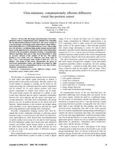
The LCSS has already been studied by Jon W. Mark [1]. In [4], authors have shown that ADC based upon LCSS has a reduced activity and thus allows power saving and noise reduction compared to Nyquist ADCs. An M-bit resolution AADC has 2M - 1 quantization levels which are disposed according to the input signal amplitude dynamics. In the studied case the quantization levels are regularly spaced. A sample is captured only when the input analog signal (x(t)) crosses one of these predefined levels. The samples are not uniformly spaced in time because they depend on the signal variations as it is clear from Figure 1. X(t) Xn-1

Xn

q

1. CONTEXT OF THE STUDY

tn-1

tn

dtn

©2007 EURASIP

Figure 1: Level-crossing sampling scheme A condition for proper reconstruction of non-uniformly sampled signals has been discussed in [5].In [5], Beutler showed that the reconstruction of an original continuous signal is possible, if the average sampling frequency F of the non-uniformly sampled signal is greater than twice of the input signal bandwidth (fmax). This condition can be expressed mathematically by F > 2 f max . According to [2], in the case of LCSS, the number of samples is directly influenced by the resolution of AADC. For an M-bit resolution AADC, the average sampling frequency of a signal can be calculated by exploiting its statistical characteristics. Then an appropriate value of M can be chosen in order to respect the Beutler’s criterion. 3. PROPOSED FILTERING TECHNIQUE Block diagram of the proposed filtering technique is shown in Figure 2. This technique is splitted into two filtering cases explained in Sections 3.3.1 and 3.3.2 respectively. Reference Filtrer

Reference FIR Filtrer

Decimater Of Reference Filter Impluse Response

Filtering Case Selector

Filter Coefficients Scalar

Reference Filter Sampling Frequency (Fref)

D ecim ated & S caled R eference Filtrer

The motivation of this work is to contribute in the development of smart mobile systems. The goal is to reduce their size, cost, power consumption, processing noise and electromagnetic emission. This can be done by smartly reorganizing their associated signal processing theory and architecture. The idea is to combine the signal event driven processing with the clock less circuit design in order to reduce the system dynamic activity. Mostly the systems are processing signals with interesting statistical properties, but the Nyquist signal processing architectures do not take full advantage of such properties. These systems are highly constrained due to the Shannon theory especially in the case of signals such as electro-cardiograms, speech, seismic signals etc. which are almost always constant and vary sporadically only during brief moments. This condition causes a large number of samples without any relevant information, a useless increase of system activity and so a useless increase of system power consumption. This problem can be resolved by employing a smart sampling scheme, captures only the relevant information from the incoming signal. The idea is to realize a signal event driven sampling scheme, based on signal amplitude variations. This sampling scheme drastically reduces the activity of the post processing, analysis or communication chain because it only captures the relevant information. It is based on “level-crossing” that provides a non-uniform time repartition of the samples. In this context an AADC (Asynchronous Analog to Digital Converter) [2] based on LCSS (Level Crossing Sampling Scheme) [1] has been designed. Algorithms for processing [3 & 6] and analysis [7 & 8] of the non-uniformly spaced out in time sampled data obtained with AADC have also been developed. The focus of this work is to develop an efficient FIR filtering technique. The idea is to adapt the sampling rate and the filter order by following the variations of the incoming signal. An efficient solution is proposed by combining the features of both non-uniform and uniform signal processing tools.

Di Band Pass Filtered Analog Signal AADC x(t)

Non-Uniformly Sampled Signal (xn,tn)

ASA

Selected Signal (xs,ts) Resampling Frequency (Frsi)

Resampler

Uniformly Sampled Signal (xrn)

FIR Filter for the

itth Selected widow

Filtered Signal (xfn)

Figure 2: Block Diagram of the proposed filtering technique,‘____’ represents the common blocks and signal flow used in both filtering cases,‘……..’ represents the signal flow used only in case 1 and ‘----’ represents the blocks and signal flow used only in case 2

2139


3.1. AADC + ASA For a non-uniformly sampled signal obtained at the output of an AADC, the sampling instants (according to [1]) are defined by Equation 1. (1) t n = t n −1 + dt n . In Equation 1, tn is the current sampling instant, tn-1 is the previous one and dtn is the time delay between the current and the previous sampling instant, as shown in Figure 1. Let δ be the processing delay of AADC for one sample point. For proper signal acquisition the x(t) must satisfy the “tracking condition” [2] given by Expression 2. In Expression 2, q is the quantum of AADC and is defined by Equation 3. dx (t ) q . ∆ x (t ) . (2) (3) ≤ q = dt δ 2 M − 1 In Equation 3, ∆x(t) represents the amplitude dynamics of x(t) and M represents the resolution of AADC. AADC has a finite bandwidth so in order to respect the Beutler’s criteria [5] and the tracking condition [2], a band pass filter with pass-band [fmin ; fmax] is employed at the input of AADC. The relevant (active) parts of the non-uniformly sampled signal are selected and windowed by ASA (Activity Selection Algorithm). This algorithm has been implemented by employing the values of dtn (Equation 1). The complete procedure of activity selection has been explained in [8]. ASA displays interesting features with LCSS which are not available in the classical case. It correlates length of the selected window with the signal activity. In addition, it also provides an efficient reduction of the phenomenon of spectral leakage in case of transient signals. This is done by minimizing the signal truncation problem with a simple and efficient algorithm instead of a smoothening window function (used in the classical scheme) [8]. 3.2. Adaptive Rate Sampling In case of AADC the sampling is triggered when the input signal crosses one of the pre-specified threshold levels. As a result, the temporal density of the sampling operation is correlated to the input signal variations. The relevant signal parts are locally over-sampled in time [3]. More the signal varies rapidly more it crosses thresholds in a given time period. This is the reason of local over-sampling in time of relevant signal parts. Contrary no sample is taken for the static signal parts. The approach is especially well suited for the low activity sporadic signals. Hence for such kind of signals the average sampling frequency remains less than the required sampling frequency for the classical scheme, performing the same operation. This smart sampling reduces the system activity and at the same time improves the accuracy of signal acquisition. ASA selects and windows relevant parts of the non-uniformly sampled signal obtained at the output of AADC. The selected data obtained at the output of ASA can be used directly for further digital processing. However in the studied case it is required to uniformly resample the selected data. So there will be an additional error due to this transformation. Nevertheless, prior to this transformation, one can take advantage of the inherent over-sampling of the relevant signal parts in the system. Hence it adds to the accuracy of postresampling process. The NNR (nearest neighbour resampling) interpolation is employed for data resampling. The reasons of inclination towards NNR interpolation are discussed in [8 & 11]. The resampling frequency (Frsi) of each selected window obtained at the output of ASA can be specific depending upon the window length (in seconds) and the signal slope lying within this window [8]. The value of Frsi for the ith selected window can be calculated by using the following equations. Ni . (4) (5) Tsi = t max i − t min i . Frs i = Ts i

©2007 EURASIP

In Equation 4, tmaxi and tmini are the final and the initial times of the ith selected window. These parameters describe the window length (Tsi) in seconds. In Equation 5, Ni is the number of samples lying in the ith selected window, depends upon the signal slope lying within this window [8]. 3.3. Adaptive Rate Filtering The proposed filtering technique is a smart alternative of the multirate filtering [9 & 10]. It achieves computational efficiency which is not attainable with the classical FIR filtering. It is known that for fixed design parameters (cut-off frequency, transition-band width, pass-band and stop-band ripples) the FIR filter order varies as a function of the operational sampling frequency. For high sampling frequency the order is high and vice versa. Thus computational gain can be achieved by adapting the sampling frequency and the filter order by following the input signal variations. In the classical signal processing the input signal is sampled at a fixed sampling frequency, regardless of its activity. A unique (fixed order) FIR filter is employed to filter this sampled signal. Contrary in case of the proposed filtering technique the sampling frequency and the filter order both are adapted by following the incoming signal variations. The computational gain over the classical filtering is achieved by realising the adaptive rate sampling (only relevant samples to process) along with the adaptive filter order (only relevant number of operations per output sample). The idea is to offline design a reference FIR filter by taking into account the incoming signal statistical characteristics and the application requirements. In the studied case the reference filter is designed by taking into account the bandwidth (fmax) of x(t). The reference filter is designed for a reference sampling frequency (Fref), satisfying the Nyquist criteria for x(t). It can be expressed mathematically by Expression 6. (6) F ref ≥ 2 × f max . The reference filter impulse response (hk) is sampled at Fref during offline processing. Here k represents the index of the reference filter coefficients. Fref and the resampling frequency of the ith selected window (Frsi) should match in order to perform a proper filtering operation. During online processing Fref and Frsi remain the same if they are already equal. Otherwise, the difference between Fref and Frsi leads to two different filtering cases, explained below. The combine flowchart of both filtering cases is shown in Figure 3. IF Yes

Frsi > Fref

Frsi = Fref

IF No

Di = Fref /Frsi IF No

Di is integer

Frsi = Frsi x (Di / floor(Di))

IF Yes

Frsi

Figure 3: Combine flowchart of both filtering cases, ‘____’ represents the common block used in both cases, ‘……..’ represents the block and signal flow only used in case 1 and ‘-----’ represents the blocks and signal flow only used in case 2 3.3.1. Filtering case 1 This case is true if Frsi is greater than Fref. In this case Fref remains the same and Frsi is decreased to match it to Fref. For case 1, Frsi (calculated by Equation 5) is higher than the overall Nyquist frequency of x(t). The upper limit on the Frsi is employed by the Bernstein’s inequality [2], given by Expression 7. In Expression 7, ∆x(t)

2140


is the amplitude dynamics of x(t). Here ∆x(t) is adapted to match to the amplitude range of AADC. The term on left hand side is the slope of x(t) and fmax is the bandwidth of x(t). Thus for an M-bit resolution AADC the highest sampling frequency (Fsmax) occurs for a pure sinusoid of frequency fmax and amplitude ∆x(t) and can be calculated by employing Equation 8. M dx ( t ) ≤ 2 .π .∆ x ( t ). f max . (7) Fs max = 2. f max .(2 − 1) . (8) dt Fsmax applies the upper limit on Frsi. Once the data is sampled by AADC and windowed by ASA, Frsi can be reduced by simply assigning Frsi = Fref. This is done in order to resample the selected data lying in the ith selected window closer to the Nyquist frequency. It avoids the unnecessary interpolations during the data resampling process of the ith selected window. It also avoids the processing of unnecessarily samples from the system. Therefore improves the computational gain of the proposed filtering process. 3.3.2. Filtering case 2 This case is valid if Fref is greater than Frsi. In this case it appears that the data lying in the ith selected window may be resampled at a frequency which is less than the overall Nyquist frequency of x(t).Therefore it can cause aliasing. The sampling rate of AADC varies according to the slope of x(t). A high frequency signal part has a high slope and AADC samples it at a higher rate. Hence a signal part with only low frequency components can be sampled by AADC at an overall sub-Nyquist frequency of x(t). But still this signal part is locally over-sampled in time with respect to its local bandwidth. This statement is valid as far as the amplitude dynamics of this signal part are adapted to match the amplitude range of AADC. It makes the relevant signal part to usually cross all thresholds (more than one) of AADC so it is locally over-sampled in time. This statement is further illustrated with the results summarised in Table 3. Hence there is no danger of aliasing when the low frequency relevant signal parts are locally over-sampled at overall subNyquist frequencies. In case 2, hk is decimated in order to keep the sampling frequency of the decimated filter coherent with Frsi. The decimation factor Di can be specific for each selected window depending upon Frsi. Various methods can be adapted to deal with the fractional Di and to keep the sampling frequency of the decimated filter coherent with Frsi. The employed method is depicted in Figure 3. From Figure 3 it is clear that Di and Frsi are correlated. First Di is calculated by using Frsi. Then a decision is made on the basis of Di, weather an adjustment of Frsi is required or not. If Di is an integer keep the same Frsi. If Di is not an integer, make an increment in Frsi depending upon the fractional part of Di and then the Di is recalculated for this new Frsi. This fulfils both above stated goals of keeping Di as an integer and the sampling frequency of the decimated filter coherent with Frsi. A simple decimation leads to a reduction of filter’s energy which will lead to an attenuated version of the filtered signal. Di is a good approximate of ratio between energy of the original (reference) filter and of the decimated filter (decimated for the ith selected window). Hence this effect of decimation is compensated by scaling the coefficients of the decimated filter with Di. The process of obtaining the decimated and scaled filter for the ith selected window from the reference one is shown mathematically by Equations 9 and 10. (9) (10) hd i , j = h D k . hwi , j = hd i , j × Di .

then the length of hdi,j is Pi = A/Di. The process of scaling the hdi,j in order to obtain the decimated and scaled impulse response (hwi,j) for the ith selected window is clear from Equation 10. 4. ILLUSTRATIVE EXAMPLE In order to illustrate the proposed filtering technique an input signal shown on the left part of Figure 4 is employed. Its total duration is 20 seconds and consists of three active parts. The summery of signal active parts is given in Table 1.

©2007 EURASIP

Signal Components

Length (Sec)

First Second Third

0.5.sin(2.π.20.t) + 0.4.sin(2. π.1000.t) 0.45.sin(2. π.10.t) + 0.45.sin(2. π.150.t) 0.6.sin(2. π.5.t) + 0.3.sin(2. π.100.t)

0.5 1.0 1.0

Table 1: Summary of the input signal active parts Table 1 shows that the input signal is band limited up to 1 kHz. This signal is sampled by employing a 3-bit resolution AADC. As M = 3 so the highest possible sampling frequency (Fsmax), calculated by Equation 8 is 14 kHz. The non-uniformly sampled signal obtained with AADC is selected and windowed by ASA. For this example the reference (initial) window length is chosen equal to 1 second [8]. The three selected windows obtained with ASA, centred on each active part of the input signal are shown on the right part of Figure 4.

Figure 4: Input signal (left) and the selected signal (right) Table 1 shows that each active part of the signal has a low and high frequency component. In order to filter the high frequency component of each signal activity a low pass reference FIR filter is implemented by using the standard Parks-McClellan algorithm. The reference filter parameters are given in Table 2. Cut-off Freq (Hz) 30

Transition Band (Hz) 30~80

Pass Band Ripples -25 (dB)

Stop Band Ripples -80 (dB)

Fref ( Hz) 2500

A 127

Table 2: Summary of the reference filter parameters In Table 2, A represents the order of the designed reference filter. Fref is the reference sampling frequency for which the reference filter is designed. As x(t) is band limited to 1 kHz so the Fref is chosen equal to 2.5 kHz in order to satisfy the condition given by Expression 6. Parameters of each selected window, obtained with ASA are summarized in Table 3. Selected Window First Second Third

i

According to Equation 9 the decimated filter impulse response (hdi,j) for the ith selected window is obtained by picking every Dith coefficient from the reference filter impulse response (hk). Here k and j represents the indexes of the impulse responses of the reference filter and of the decimated filter respectively. If the length of hk is A

Active Part

Tsi (Sec) 0.4998 0.9995 0.9992

Ni (Samples) 3000 1083 460

Frsi (Hz) 6000 1083 460

Fref (Hz) 2500 2500 2500

Filtering case 1 2 2

Table 3: Summary of parameters of each selected window Table 3 exhibits the interesting features of the proposed filtering technique. Ni and Frsi represent the sampling frequency adaptation by following the slope of x(t). It is achieved due to the smart fea-

2141


tures of AADC and ASA. It is also clear from Ni that the relevant signal parts are over-sampled locally in time like any harmonic signal [3]. Tsi in Table 3 exhibits the dynamic feature of ASA which is to correlate the reference window length with the signal activity lying in it. Contrary in the classical case, the windowing process does not select only the active parts of the sampled signal. Moreover the reference window length remains static and is not able to adapt according to the signal activity lying within the window. For this studied example the reference window length is chosen equal to 1 second. Hence in the classical case, it will lead to twenty 1-second windows for the whole signal span (20 Sec). It follows that the system has to process more than the relevant information part. The decimation factor (Di), the filter order (Pi) and the adjusted resampling frequency (Frsi), for each selected window is summarized in Table 4. Selected Window First Second Third

Filtering case 1 2 2

Frsi (Hz) 6000 1083 460

Adjusted Frsi (Hz) 2500 1250 500

Di

Pi

x 2 5

127 64 26

Spectrum of 3rd Selected Window (Uniform case) 0.4

0.3 0.3

0.25 0.2

0.2

0.15

Amplitude Axis

0.1

0.1

0.05 0

0

100

200

300

400

500

0

0

Zoom of the Spectrum (Filtering case 2) 0.3

Relative Error = 0.4%

500

1000

1500

2000

2500

Zoom of the Spectrum(Uniform case) 0.3

0.28 0.28

0.26 0.24

0.26

0.22 0.2

0.24

0.18 5

10

15

20

25

0.22 30 Frequency Axis

5

10

15

20

25

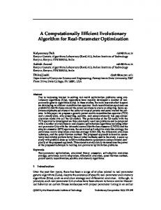
Figure 5: Spectrum of the filtered signal and its zoom obtained with the proposed filtering technique (top and bottom left respectively) and obtained with the classical filtering technique (top and bottom right respectively)

Table 4: Di ,Pi and adjusted Frsi, for the ith selected window For the 1st selected window filtering case 1 is valid. So Frs1 is reduced by assigning Frs1 = Fref. This reduction of Frs1 has two following benefits. First it avoids the needless interpolations during the data resampling process of the 1st selected window. Secondly it avoids the processing of excessive samples from the system. Hence it adds to the computational efficiency of the proposed filtering technique. In case 1, hk remains unaltered so there is no need to calculate D1. For the 2nd and the 3rd selected windows the filtering case 2 is valid. So hk is decimated with D2 and D3 for the 2nd and the 3rd selected windows respectively. P2 and P3 in Table 4 represent the adaptation of reference filter order for the 2nd and the 3rd selected windows. D2 and D3 are used later on to scale the impulse responses of decimated filters hd2,j and hd3,j respectively. This scaling is applied to keep the energy of decimated filters at the same level to that of the original (reference) filter. The adaptation of hk for the 2nd and the 3rd selected windows is another advantage of the proposed technique. It is achieved due to the appealing feature of ASA. Contrary, in the classical case the filter remains time invariant and has to be designed for the worst situation. In this example the input signal is band limited to 1 kHz. Therefore if the sampling frequency is chosen equal to 2.5 kHz in order to respect the Shannon theorem then for the same filter parameters (Table 2), Parks-McClellan algorithm design gives a 127th order FIR filter. In the classical case the signal is sampled at a fixed sampling frequency (2.5 kHz), regardless of its activity. Hence a fixed order filter (H = 127) is employed for the whole signal span. That causes a useless system activity. The activity lying in the 3rd selected window is filtered by applying the proposed filtering technique and the classical one. In order to make a comparison of filtering quality the spectra of filtered signals obtained with the proposed and the classical filtering techniques are calculated. Spectra of the filtered signals and their zooms obtained with the proposed and the classical filtering techniques are shown in the left and the right parts of Figure 5 respectively. Figure 5 shows that a relative error of 0.4% occurs between the results obtained with the proposed and the classical filtering techniques. It shows that for the 3rd selected window decimation of the reference filter leads to a loss of quality. The measure of this quality loss can be used to decide the upper bound on the decimation factor (Di). By performing offline calculations the maximum value of Di can be decided for which the decimated and scaled filter provides filtering with an acceptable level of accuracy. The level of accuracy is application dependent.

©2007 EURASIP

Spectrum of 3rd Selected Window (Filtering case 2)

5. COMPUTATIONAL COMPLEXITY This section compares the computational complexity of the proposed filtering technique with the classical one. The complexity evaluation is made by considering the number of online operations executed to perform the algorithm. It is known that in the classical case the incoming signal is sampled at a fixed sampling frequency. In this case a time invariant, fixed order filter is employed to filter the sampled data. As for an H order FIR filter, H multiplications and H additions are computed for each output sample. The total computational complexity C1 for Nu (number of uniform) samples can be calculated by employing Equation 11. In the proposed filtering technique, the sampling frequency and the filter order both are not fixed and are adapted for each selected window according to the slope of x(t). In comparison to the classical case this approach locally requires some extra operations in each selected window. Filtering case selection is the first online operation performed by the proposed filtering technique. It requires one comparison between Fref and Frsi. If case 1 is true then the reference filter impulse response (hk) remains the same. Contrary in case 2, hk is decimated. The data resampling operation is required in both cases before filtering. In case 1, resampling is performed at a reduced Frsi. On the other hand in case 2, it is performed at the same or an increased Frsi (recall Figure 3). The NNR interpolator is employed to resample the non-uniform selected data. This interpolator requires only a comparison operation for each resampled observation. Therefore the interpolator performs Ni comparisons, where Ni represents the total number of samples lying in the ith selected window. In addition to this, filtering case 2 requires some additional operations. In case 2, it is required to decimate hk. Therefore Di is calculated for the ith selected window. The calculation of Di requires seven operations for the worst situation, three divisions, one multiplication, two comparisons and one floor operation as shown in Figure 3. In order to make a complexity comparison the operation count for the worst situation is taken into account. Decimation process of the reference filter for the ith selected window has a negligible complexity as compare to operations like addition or multiplication. This is the reason that the complexity of the decimator is not taken into consideration. Moreover, it is required to scale the impulse response of the decimated filter by Di. The filter coefficients scalar performs Pi multiplications; here Pi represents the order of the deci-

2142


mated filter for the ith selected window. The combined computational complexity C2 of the proposed filtering technique for both filtering cases is given by Equation 12. . (11) C = H .N + H .N 1

123u Additions

C 2=

123u

Multiplica tions

L

+ 1{ + ∑ ( N i + 3) + Pi .N i + (Pi .N i + β .Pi ) . (12) 1 424 3 123 14 4244 3 Floor i =1 Divisions 3{

Comparisons

Additions

Multiplications

In Equations 12, β is a multiplying factor and its value is 0 for case 1 and 1 for case 2. The parameter i = {1, 2, 3,…., L} represents the index of the selected window. The computational gain of the proposed filtering technique over the classical one can be calculated by employing Equation 13.

G=

C1 = C2

H . N u + H .N u

.

(13)

L

3 + 1 + ∑ ( N i + 3) + Pi .N i + ( Pi .N i + β .Pi ) i =1

From Equations 11 and 12 it is clear that addition and multiplication are the common operations between the classical and the proposed filtering techniques. The operations like comparison, division and floor are uncommon between them and are required only in the proposed filtering technique. Because of these uncommon operations the computation comparison between the proposed and the classical filtering techniques is not straightforward. In order to make them approximately comparable the following assumptions are made. *Comparison has same processing cost as that of an addition. *Division and floor operations are very small in number as compare to the addition, multiplication and comparison operations, so can be ignored during computation evaluation. By following these assumptions, comparisons are merged into additions and divisions and floor are neglected during the complexity evaluation process. The computational gain of the proposed filtering technique over the classical one is calculated for the results of illustrative example, for different time spans of x(t). The results are summarized in Table 5. Time Span (Sec) Ts1 Ts2 Ts3 Total signal span (20)

Gain in Additions 1.98 3.90 23.5 24.9

Gain in Multiplications 2 3.97 24.42 25.2

Table 5: Summary of processing gain of the proposed filtering technique over the classical one The adjusted value of Frs1 is equal to the sampling frequency in the classical case (Table 4). Yet 1.9 & 2 times gains are achieved in additions and multiplications respectively, for the 1st selected window. This is due to the dynamic feature of ASA which is to correlate the window length with the signal activity lying in it (0.5 Sec). Contrary, in the classical case the window length remains static (1 Sec) and system has to process extra samples. Table 5 shows 24.9 & 25.2 times gains in additions and multiplications respectively for the whole signal span (20 sec). This gain is achieved by employing the joint benefits of AADC, ASA and resampling. As they allow to adapt the sampling frequency and the filter order by following the incoming signal variations. 6. CONCLUSIONS A new adaptive rate filtering technique is proposed. This technique is well suited for low activity sporadic signals like electrocardiograms, speech, seismic signals, etc. A reference filter is designed offline by taking into account the input signal bandwidth and the application requirements. The proposed technique is splitted into

©2007 EURASIP

two filtering cases. A complete methodology of firstly choosing the appropriate filtering case for the ith selected window and then adjusting Frsi or hk depending upon the validity of case 1 or case 2 respectively has been demonstrated. It shows how the data resampling rate or the reference filter order is smartly adapted for each selected window by following the input signal variations. The computational complexity of the proposed adaptive rate filtering technique is deduced collectively for both filtering cases. A method to make an approximate computation comparison between the proposed and the classical filtering techniques is described. The comparison is made by using the results of an illustrative example. The results show 24.9 times gain in additions and 25.2 times gain in multiplications of the proposed filtering technique over the classical one. It shows that the proposed filtering technique leads to a significant reduction of the total number of operations. This reduction in operations is achieved by combining the adaptive rate sampling (reduce the number of samples to process) along with adaptive rate filtering (reduce the number of operations per output sample). The decimation of reference filter is required in filtering case 2. The complete procedure of decimating and scaling the pre-calculated reference filter during online computation is demonstrated. The decimation of reference filter reduces the quality of the decimated filter as compared to the reference one. The upper bound on decimation factor can be determined by offline calculations, for which the decimated and scaled filter gives response with an acceptable level of accuracy. Moreover for applications where high quality filtering is required, an appropriate filter can be calculated directly online for each selected window at the cost of an increased computational load. REFERENCES [1] J.W. Mark and T.D. Todd, “A nonuniform sampling approach to data compression” IEEE Transactions on Communications, vol. COM-29, pp. 24-32, January 1981. [2] E. Allier, G. Sicard, L. Fesquet and M. Renaudin, “A new class of asynchronous A/D converters based on time quantization”, ASYNC'03, pp.197-205, Vancouver, B.C, Canada, May 2003. [3] F. Aeschlimann, E. Allier, L. Fesquet and M. Renaudin, “Asynchronus FIR filters, towards a new digital processing chain”, ASYNC'04, pp. 198-206, Crete, Greece, April 2004. [4] N. Sayiner, H.V. Sorensen and T.R. Viswanathan, “A LevelCrossing Sampling Scheme for A/D Conversion”, IEEE Transactions on Circuits and Systems II, vol. 43, pp. 335-339, April 1996. [5] F.J. Beutler, “Error free recovery from irregularly spaced samples”, SIAM Review, vol. 8, pp. 328-335, 1996. [6] S. M. Qaisar, L. Fesquet, M. Renaudin “Adaptive rate filtering for a signal driven sampling scheme”, ICASSP’07, April 15-20, 2007, Honolulu, Hawaii, USA. [7] F. Aeschlimann, E. Allier, L. Fesquet and M. Renaudin “Spectral analysis of Level Crossing Sampling Scheme”, International Workshop on Sampling theory and application SAMPTA, Samsun, Turkey, 10-15 July 2005. [8] S. M. Qaisar, L. Fesquet, M. Renaudin “Spectral analysis of a signal driven sampling scheme”, EUSIPCO 2006, September 4-8, 2006, Florance Italy. [9] Shuni Chu, Burrus, C. “Multiate filter designs using comb filters”, IEEE transaction on Circuits and Systems, vol. 31, PP. 913924, November 1984. [10] M. Vetterli, M. “A theory of multirate filter banks”, IEEE transaction on Acoustic, Speeh and Signal Processing, vol. 35, March 1987. [11] S. de Waele and P.M.T.Broersen “Time domain error measures for resampled irregular data”, IEEE Transactions on Instrumentation and Measurements, pp.751-756, Venice, Italy, May 1999.

2143