1.2 Space Vehicle Navigation. 3. 1.3 Estimation Algorithms and Non-linearity ...... [150] NASA, âSpaceX CRS-5 Fifth Commercial Resupply Services Flight to the ...
Computationally Efficient Non-linear Kalman Filters for On-board Space Vehicle Navigation by Sanat Kumar Biswas
A Thesis submitted in fulfillment of the requirements for the Degree of Doctor of Philosophy
School of Electrical Engineering and Telecommunications Faculty of Engineering July 2017
iii
PLEASE TYPE THE UNIVERSITY OF NEW SOUTH WALES Thesis/Dissertation Sheet Surname or Family name: Biswas First name: Sanat
Other name/s: Kumar
Abbreviation for degree as given in the University calendar: PhD School: Electrical Engineering and Telecommunications
Faculty: Engineering
Title: Computationally Efficient Non-linear Kalman Filters for On-board Space Vehicle Navigation
Abstract 350 words maximum: (PLEASE TYPE) The Extended Kalman Filter (EKF) is the most popular non-linear estimation algorithm due to its computational efficiency. It is frequently used in on-board space vehicle navigation. However, for highly non-linear applications, due to the degraded performance of the EKF, the Unscented Kalman Filter (UKF) was proposed to deliver better accuracy. The UKF requires more computational time than the EKF. This dissertation proposes two computationally efficient UKFs called the Single Propagation Unscented Kalman Filter (SPUKF) and the Extrapolated Single Propagation Unscented Kalman Filter (ESPUKF), which predict the state vector by propagating only one sample state vector. These new algorithms are accurate to the first and second order Taylor series terms. Using theoretical analysis and several example space applications with radar and Global Navigation Satellite System (GNSS) observations, it is demonstrated that these new techniques can reduce the processing time of the UKF by up to 90%. The Unscented-type Kalman Filters have advantages when the problem is “highly” non-linear. However, the relationship between non-linearity and the UKF performance improvement over the EKF had not been thoroughly investigated. A mathematical relation between a quantitative measure of non-linearity and the UKF performance relative to the EKF is presented in this dissertation. The performance improvement the UKF can attain is shown to depend on the non-linearity of the system and the measurements. Several non-linear problems are examined to verify the relation. This analysis provides a quantitative approach to selecting between the UKF and the EKF. The effect of the Position Dilution of Precision (PDOP) of GNSS observations on the EKF and UKF performance in space vehicle navigation was also studied. Using the least square method, the position standard deviation has a linear relation with the PDOP. It is shown that, in the Kalman Filter framework, the position standard deviation has a hyperbolic relation with the PDOP. The new algorithms will facilitate accurate on-board implementation of estimation algorithms for highly non-linear space vehicle navigation problems. The analytical results relating the Kalman Filter performance, non-linearity and PDOP enable structured selection between the EKF and UKF. Declaration relating to disposition of project thesis/dissertation I hereby grant to the University of New South Wales or its agents the right to archive and to make available my thesis or dissertation in whole or in part in the University libraries in all forms of media, now or here after known, subject to the provisions of the Copyright Act 1968. I retain all property rights, such as patent rights. I also retain the right to use in future works (such as articles or books) all or part of this thesis or dissertation. I also authorise University Microfilms to use the 350 word abstract of my thesis in Dissertation Abstracts International (this is applicable to doctoral theses only).
…………………………………………………………… Signature
……………………………………..……………… Witness Signature
……….……………………...…….… Date
The University recognises that there may be exceptional circumstances requiring restrictions on copying or conditions on use. Requests for restriction for a period of up to 2 years must be made in writing. Requests for a longer period of restriction may be considered in exceptional circumstances and require the approval of the Dean of Graduate Research. FOR OFFICE USE ONLY
Date of completion of requirements for Award:
Originality Statement I hereby declare that this submission is my own work and to the best of my knowledge it contains no materials previously published or written by another person, or substantial proportions of material which have been accepted for the award of any other degree or diploma at UNSW or any other educational institution, except where due acknowledgement is made in the thesis. Any contribution made to the research by others, with whom I have worked at UNSW or elsewhere, is explicitly acknowledged in the thesis. I also declare that the intellectual content of this thesis is the product of my own work, except to the extent that assistance from others in the project’s design and conception or in style, presentation and linguistic expression is acknowledged.
Signed
Date
v
Copyright Statement I hereby grant the University of New South Wales or its agents the right to archive and to make available my thesis or dissertation in whole or part in the University libraries in all forms of media, now or here after known, subject to the provisions of the Copyright Act 1968. I retain all proprietary rights, such as patent rights. I also retain the right to use in future works (such as articles or books) all or part of this thesis or dissertation. I also authorize University Microfilms to use the 350 word abstract of my thesis in Dissertation Abstract International (this is applicable to doctoral theses only). I have either used no substantial portions of copyright material in my thesis or I have obtained permission to use copyright material; where permission has not been granted I have applied/will apply for a partial restriction of the digital copy of my thesis or dissertation.
Signed
Date
vii
Authenticity Statement I certify that the Library deposit digital copy is a direct equivalent of the final officially approved version of my thesis. No emendation of content has occurred and if there are any minor variations in formatting, they are the result of the conversion to digital format.
Signed
Date
ix
To my parents and beloved wife
xi
Abstract The Extended Kalman Filter (EKF) is the most popular non-linear estimation algorithm due to its computational efficiency. It is frequently used in on-board space vehicle navigation. However, for highly non-linear applications, due to the degraded performance of the EKF, the Unscented Kalman Filter (UKF) was proposed to deliver better accuracy. The UKF requires more computational time than the EKF. This dissertation proposes two computationally efficient UKFs called the Single Propagation Unscented Kalman Filter (SPUKF) and the Extrapolated Single Propagation Unscented Kalman Filter (ESPUKF), which predict the state vector by propagating only one sample state vector. These new algorithms are accurate to the first and second order Taylor series terms. Using theoretical analysis and several example space applications with radar and Global Navigation Satellite System (GNSS) observations, it is demonstrated that these new techniques can reduce the processing time of the UKF by up to 90%. The Unscentedtype Kalman Filters have advantages when the problem is “highly” non-linear. However, the relationship between non-linearity and the UKF performance improvement over the EKF had not been thoroughly investigated. A mathematical relation between a quantitative measure of non-linearity and the UKF performance relative to the EKF is presented in this dissertation. The performance improvement the UKF can attain is shown to depend on the non-linearity of the system and the measurements. Several non-linear problems are examined to verify the relation. This analysis provides a quantitative approach to selecting between the UKF and the EKF. The effect of the Position Dilution of Precision (PDOP) of GNSS observations on the EKF and UKF performance in space vehicle navigation was also studied. Using
xiii
xiv the least square method, the position standard deviation has a linear relation with the PDOP. It is shown that, in the Kalman Filter framework, the position standard deviation has a hyperbolic relation with the PDOP. The new algorithms will facilitate accurate on-board implementation of estimation algorithms for highly non-linear space vehicle navigation problems. The analytical results relating the Kalman Filter performance, non-linearity and PDOP enable structured selection between the EKF and UKF.
Acknowledgment It is a pleasure to thank the many individuals whose support and guidance have made this thesis possible. First and foremost, I would like to express my profound gratitude to my supervisor, Professor Andrew Graham Dempster for providing me an opportunity to research under his supervision. He always encouraged me to think independently rather than directing me to what to do next. His supervision transformed the PhD research into a fascinating journey to finding answers to some fundamental problems. I will always remain thankful to Professor Dempster for providing me research assistantship and providing me opportunities to attend several conferences. My research would have been impossible without his guidance, support and encouragement. My equally sincere thanks to my co-supervisor Dr. Li Qiao for her support and advice. Her guidance helped me to stay focused on a particular research topic and her accurate feedback has improved my research. I am grateful to both of my supervisors for all the trust they have put in my work over the past years. Heartfelt thanks go to Dr. Mazher Choudhury, Dr. Eamonn Glennon and Dr. Joon Wayn Cheong at the Australian Centre for Space Engineering Research (ACSER) for sharing their expertise which helped me to design and execute Namuru and Kea receiver related experiments using SPIRENT. I would also like to thank Cheryl Brown, Administrative Officer of ACSER for all administrative supports. My sincere thanks to the Annual Progress Review Panel members: Dr. Elias Aboutanios and Dr. Julien Epps for their advice and feedback which enriched my research work. I am thankful to my friend Dr. Muhammad Ali Nawaz for all the scientific and
xv
xvi technological discussions we used to have during leisure. From many of these informal discussions, I received some insight which helped me to look at my research problems from different perspectives. I would like to thank all my friends and colleagues of Signal Processing Group in the School of Electrical Engineering and Telecommunications for their various supports which helped me to overcome many difficulties in last four years. I am also grateful to my M.Tech supervisor Professor Hari B. Hablani. I learned many important attributes of academic research under his supervision which accelerated my progress during PhD. During my PhD, I enjoyed the luxury of getting married. My wife, Shyamashree Biswas has been immensely patient with me and she has been by my side, experienced all the ups and downs I had gone through. I would like to thank her for her unwavering love, support and encouragement. I am profoundly grateful to my parents who have sacrificed a lot so that I can pursue my dreams. My father, Swapan Biswas has influenced and inspired me to choose a research career. His ideals have always guided me towards the right path. My mother, Suprova Biswas was my first teacher and she single-handedly tutored me till 10th standard. Her teaching had laid the foundation of my education. There are no proper words to convey my deepest gratitude to my parents. This thesis would not have been possible without their constant support and encouragement.
Contents Abstract
xiii
Acknowledgment
xv
List of figures
xxiii
List of tables
xxv
Acronyms and Symbols
xxvii
Chapter 1 Introduction
1
1.1
Space Vehicle Classification
2
1.2
Space Vehicle Navigation
3
1.3
Estimation Algorithms and Non-linearity
3
1.4
Motivation and Objectives
4
1.5
Contributions
6
1.6
Structure of the Thesis
7
1.7
List of Publications
9
Chapter 2 On-board Space Vehicle Navigation and Related Works
11
2.1
Introduction
12
2.2
Reference Frames
12
2.3
Space Vehicle Dynamics
14
2.3.1
Launch Vehicle Dynamics
14
2.3.2
Low Earth Orbit Satellite Dynamics
16
2.3.3
Re-entry Vehicle Dynamics
18
2.4
2.5
Observations
20
2.4.1
Radar Observations
21
2.4.2
GNSS Observations
22
Estimation Algorithms
26
2.5.1
Generic non-linear system and measurement
32
2.5.2
Extended Kalman Filter
33
xvii
xviii
CONTENTS 2.5.3
Unscented Kalman Filter
34
2.6
Non-linearity and the Kalman Filter
38
2.7
Summary
40
Chapter 3 Methodology and Experimental Set-ups
41
3.1
Introduction
41
3.2
Simulation Scenarios
42
3.2.1
Launch Vehicle
42
3.2.2
LEO Satellite
46
3.2.3
Re-entry Vehicle
47
3.3
Simulation of Radar Observations
52
3.4
Simulation of GNSS Observation
54
3.4.1
SPIRENT GNSS Simulator and SimGEN
54
3.4.2
UNSW Namuru V3.3 Receiver
55
3.4.3
Kea GPS Receiver
55
3.4.4
Methodology for the Launch Vehicle Simulation
56
3.4.5
Methodology for the LEO Satellite Simulation
57
3.5
Summary
Chapter 4 Fast Unscented Kalman Filters
58 59
4.1
Introduction
59
4.2
Single Propagation Unscented Kalman Filter
60
4.2.1
Error in the Mean and the Covariance
61
4.2.2
Error in State Estimation
63
4.3
Extrapolated Single Propagation Unscented Kalman Filter
66
4.4
Results
68
4.5
4.4.1
Position Estimation of Re-entry Vehicles
68
4.4.2
Position Estimation of a LEO Satellite
74
4.4.3
Launch Vehicle Trajectory Estimation
75
Summary
Chapter 5 Computation Time Analysis
85 89
5.1
Introduction
89
5.2
Computation Time of the SPUKF
92
5.3
Computation Time Reduction by the SPUKF
93
5.4
Computation Time of the ESPUKF
95
5.5
Computation Time Reduction by the ESPUKF
96
5.6
Summary
98
xix Chapter 6 Non-linearity Analysis 6.1 Introduction 6.2 Non-linearity Index 6.3 Non-linearity Index and Kalman Filter Performance 6.3.1 Hypothesis 6.3.2 Proof 6.4 Probabilistic Analysis 6.5 Verification 6.5.1 Analytical Results 6.5.2 Experimental Results 6.6 Summary
99 99 101 103 103 104 108 111 112 112 118
Chapter 7 Dilution of Precision Analysis 7.1 Introduction 7.2 Problem Formulation 7.2.1 System and Measurement Description 7.2.2 Kalman Filter Update Equations 7.3 DOP and EKF Performance 7.4 DOP and UKF Performance 7.5 Verification 7.6 Summary
119 119 120 121 122 122 124 126 132
Chapter 8 Conclusion 8.1 A Review of Thesis Contributions 8.2 Future Work 8.2.1 Outline of Potential Research in Related Fields
135 135 137 137
Bibliography
161
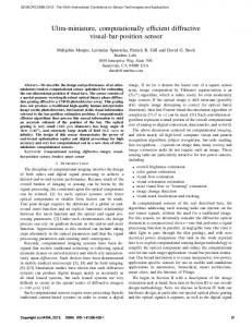
List of Figures 1.1
Major types of space vehicles
2
1.2
Flow diagram of the thesis structure
8
2.1
Reference frames
13
2.2
Launch vehicle trajectory
15
2.3
Re-entry vehicle trajectory
18
2.4
Errors in GNSS observation
23
2.5
Propagation of sigma points using conventional UT
36
3.1
Falcon 9 V1.1 trajectory for CRS-5 mission
43
3.2
Falcon 9 V1.1 velocity profile for CRS-5 mission
45
3.3
Falcon 9 V1.1 flight path angle for CRS-5 mission
45
3.4
Falcon 9 V1.1 aerodynamic coefficient for CRS-5 mission
46
3.5
Reference LEO orbit
47
3.6
Altitude profile for a vertical re-entry
48
3.7
Velocity profile for a vertical re-entry
48
3.8
Aerodynamic co-efficient profile for a vertical re-entry
49
3.9
Re-entry vehicle trajectory
50
3.10 Velocity profile of a re-entry vehicle
50
3.11 Flightpath angle profile of a re-entry vehicle
51
3.12 Aerodynamic co-efficient profile of a re-entry vehicle
51
3.13 Range observation for a vertical re-entry
52
3.14 Radar tracking geometry for a re-entry vehicle in a curved trajectory
53
3.15 Estimation using radar observations
54
3.16 Namuru V3.3 multi-GNSS receiver
55
3.17 Kea GPS receiver
55
3.18 Using external trajectory data in SPIRENT simulator
56
3.19 Simulation without GPS receiver
56
3.20 Simulation with GPS receiver
57
3.21 Simulation experiment with the LEO satellite
57
xxi
xxii
LIST OF FIGURES
4.1
Approximate sigma point propagation
60
4.2
Performance comparison of the SPUKF and ESPUKF with other estimation algorithms
69
4.3
Processing time vs. estimation error for different algorithms
70
4.4
Estimation errors for different KFs
72
4.5
Estimation errors for UKFs
73
4.6
Processing time vs. estimation error
73
4.7
Comparison of the estimated position error
74
4.8
Estimation errors of different Kalman Filters
77
4.9
Estimation error using different algorithms
78
4.10 Average error for different filters using 4 channels
79
4.11 Average error for different filters using 6 channels
80
4.12 Average error for different filters using 8 channels
81
4.13 Average error for different filters using 10 channels
81
4.14 Position error ratio for different number of GPS satellites used
82
4.15 Processing time vs. estimation error
82
4.16 Estimation errors for different UKFs with Kea GPS receiver
84
5.1
Computation efficiency improvement of the SPUKF
94
5.2
Limit of No. of state elements for which the SPUKF is more efficient than the UKF
94
5.3
Computation efficiency improvement of the ESPUKF
97
5.4
Limit of No. of state elements for which the ESPUKF is more efficient than the UKF
97
Different trajectories of the state vectors due to worst case initial conditions in 2-dimensional space
101
6.2
Variation of probability bounds
110
6.3
Relationship between the Non-linearity Indices and the UKF performance improvement
111
Non-linearity Index and normalised difference in filter errors for the reentry vehicle
113
Non-linearity Index and normalised difference in filter errors for the LEO satellite
114
6.1
6.4 6.5 6.6
Non-linearity Index of the LEO satellite dynamics in two orbital periods 114
6.7
Non-linearity Index of the GNSS observation dynamics for LEO satellite in two orbital periods
115
Non-linearity Index and normalised difference in filter errors for the launch vehicle
116
6.8
xxiii 6.9
Combined Non-linearity Index vs. relative UKF efficiency
116
7.1 7.2 7.3 7.4
Average � � PDOP variation with no. of satellites � 2 vs. P DOP σR Position error ratio for different number of satellites Average � PDOP variation with no. of satellites �
127 128 129 130
7.5 7.6 7.7
� σR
2
vs. P DOP 130 Average � � PDOP variation with no. of satellites for LEO Satellite navigation131 � σR
2
vs. P DOP for LEO Satellite navigation
131
List of Tables 2.1
Review of non-linear estimation algorithms
28
3.1 3.2
Mission and Launch Vehicle specific parameters Orbit parameters
44 46
4.1 4.2 4.3 4.4 4.5
Processing time and average altitude error for different algorithms Processing Time and average position error for different algorithms Processing time and average position error for different algorithms Performance of different filters with different number of GPS signals Processing time reduction by the new algorithms
70 75 76 83 86
6.1 6.2
Variation of bounds with Non-linearity Indices Range of γ for P > 0.8
110 112
8.1
Decision table for algorithm selection
140
xxv
Acronyms and Symbols Acronyms CKF CRLB CRS
Cubature Kalman Filter. Cramer-Rao Lower Bound. Commercial Resupply Service.
DOP DORIS
Dilution of Precision. Doppler Orbitography and Radio Positioning integrated by Satellite. Deep Space Network.
DSN ECEF ECI EKF ESPT ESPUKF
Earth Centered Earth Fixed frame. Earth Centered Inertial frame. Extended Kalman Filter. Extrapolated Single Propagation Technique. Extrapolated Single Propagation Unscented Kalman Filter.
FPE
Fokker-Planck Equation.
GDOP GEO GHF GHQ GLONASS
Geometric Dilution of Precision. Geosynchronous Orbit. Gauss-Hermite Filter. Gauss-Hermite Quadrature. Globalnaya Navigatsionnaya Sputnikovaya Sistema. Global Navigation Satellite System. Global Positioning System. Group and Phase Ionospheric Correction.
GNSS GPS GRAPHIC
xxvii
xxviii
Symbols HEO HS norm
High Earth Orbit. Hilbert-Schmidt norm.
IGS INS
International GPS Services. Inertial Navigation System.
LEO LSE
Low Earth Orbit. Least Square Estimation.
MEKF MEO
Multiplicative Extended Kalman Filter. Medium Earth Orbit.
NASA
National Aeronautics and Space Administration.
PDOP PRARE
Position Dilution of Precision. Precise Range and Range Rate Equipment.
SGHF SLR SPUKF SSUKF SSUT
Sparse-grid Gauss-Hermite Filter. Satellite Laser Ranging. Single Propagation Unscented Kalman Filter. Spherical Simplex Unscented Kalman Filter. Spherical Simplex Unscented Transform.
TDRSS
Tracking and Data Relay Satellite System.
UKF UT
Unscented Kalman Filter. Unscented Transform.
Symbols β
Elevation angle.
C c
Aerodynamic Co-efficient. Speed of light.
D
Aerodynamic drag.
xxix �E �U �Φ �ρ
HS norm of EKF error. HS norm of UKF error. Random noise in carrier-range measurement. Random noise in pseudo-range measurement.
f
Non-linear system function.
g γf
Gravitational acceleration. Flight path angle.
H ha h h
Jacobian of h. Altitude. Non-linear measurement function. Number of integration steps.
I
Ionospheric error.
Jn J
Zonal hermonics. Jacobian of f .
K k
Kalman gain. Discrete time index.
m ˙e m µe
Exhaust mass flow rate. Mass. Gravitational parameter of the Earth.
n Nm Ns ν
number of state variables in the state vector. Non-linearity Index of measurement model. Non-linearity Index of system model. Process noise vector.
ω
Measurement noise vector.
Φ P Φi
State transition matrix. Error covariance matrix. Carrier-range from the user vehicle to the navigation satellite i.
xxx
Symbols Q
Process noise covariance matrix.
R ρi r r RE
Measurement noise covariance matrix. Pseudo-range from the user vehicle to the navigation satellite i. range. Position vector. Local radius of the Earth.
σ
Standard deviation.
T θ t
Tropospheric error. Azimuth angle. time.
v v
speed. Velocity vector.
x
Down-range.
Y
State vector.
Z
Measurement vector.
Chapter 1 Introduction Contents 1.1
Space Vehicle Classification
2
1.2
Space Vehicle Navigation
3
1.3
Estimation Algorithms and Non-linearity
3
1.4
Motivation and Objectives
4
1.5
Contributions
6
1.6
Structure of the Thesis
7
1.7
List of Publications
9
Launching of Sputnik by the former Union of Soviet Socialist Republics (USSR) marked the dawn of the Space age in 1957. Apart from achieving science goals and technology demonstration, the Sputnik mission created scientific strides which resulted in lunar missions, earth observation satellites, the Global Navigation Satellite System (GNSS) and numerous interplanetary missions. With time, the fleet of satellites deployed by various nations has become essential for day to day life. Numerous space missions are conceived and executed every year for navigation [1], communication [2], remote sensing [3], weather forecasting [4], resource management [5], astronomical observation [6,7] and solar system exploration [8–11]. With these vital applications, space technology has proven to be essential infrastructure of human civilization [12]. It is anticipated that future space missions will open endless possibilities of technological advancements and shape the society of the coming age.
1
2
1.1
CHAPTER 1. INTRODUCTION
Space Vehicle Classification
Numerous types of space vehicle are constructed and designed based on mission requirements. Space vehicles can be broadly categorized in three types: • Launch Vehicle: Launch vehicles are essential for all space missions. These vehicles are used to carry payloads from ground into space. The most common type of launch vehicles are expendable Launch Vehicles. These vehicles are comprised of multiple expendable stages with solid and liquid propelled rocket engines [13]. A SpaceX Falcon 9 launch vehicle is shown in figure 1.1a.
(a) Falcon 9 Launch Vehicle [14]
(b) GPM Core Observatory satellite [15]
(c) Orion Re-entry Vehicle [16]
Figure 1.1: Major types of space vehicles
• On-orbit Vehicle: An on-orbit vehicle is inserted into a orbit around a celestial object. This type of vehicle is launched into space using a launch vehicle. Onorbit vehicles may change orbit or trajectory depending on the mission. These spacecraft can be Earth-bound or interplanetary. the majority of the on-orbit vehicles are artificial satellites of Earth and generally classified in terms of orbit altitude from sea level assuming circular orbit. Satellites which orbit Earth within the altitude range of 160 km to 2000 km are called Low Earth Orbit (LEO) satellites. Satellites residing within the altitude of 2000 km and 35786 km are called Medium Earth Orbit (MEO) satellites. Geosynchronous Orbit (GEO) satellites orbit the Earth at an altitude of 35786 km. Satellites above 35786 km altitude are called High Earth Orbit (HEO) satellites [17]. A LEO satellite is shown in figure 1.1b.
3 • Re-entry Vehicle: Re-entry vehicles are specially designed for atmospheric re-entry from outer space. These vehicles are constructed to withstand extreme aerodynamic heating and drag. These vehicles are used to transport human crews and payloads from space to Earth. These are also used as landers for robotic missions on surface of other planetary objects. The Orion re-entry vehicle is shown in figure 1.1c.
1.2
Space Vehicle Navigation
The operation of a space vehicle relies on a collection of interdependent functions: structure, power, navigation, attitude determination, guidance, control, thermal, telemetry and command, propulsion and data handling [12]. Among these vital functional segments, accurate navigation i.e. determination of the position and velocity is often crucial for the success of a space mission. Precise position and velocity information of a launch vehicle is required for insertion of a spacecraft into its orbit and for range safety [18–20]. In orbit position determination is important for station keeping, guidance and maneuvering of earth-orbiting artificial satellites and deep space-faring spacecraft [21]. For re-entry missions, position and velocity information are even more vital for proper re-entry procedures and vehicle recovery [22, 23]. Navigation of all types of space vehicles requires some input observations that are functions of position and velocity of space vehicles. Dead-reckoning, range, range rate, pointing angles and angular measurements to known celestial objects are widely used as measurements for space vehicle navigation. Position and velocity of space vehicles are estimated from these measurements using a suitable estimator.
1.3
Estimation Algorithms and Non-linearity
Estimation is the process of determining an approximation of desired quantities from incomplete or uncertain data. Estimation processes can be of two types: batch estimation and sequential estimation. In batch estimation, all the observations are processed
4
CHAPTER 1. INTRODUCTION
to estimate the desired state vector. This technique requires storage of all the observations and processing time increases as the number of observations increases [24]. Hence this method is not suitable for a real-time estimation solution. On the other hand, a sequential estimator uses observations collected at an epoch to estimate a state vector at that epoch. Of several types of sequential estimators, the Kalman Filter is designed for the state estimation of stochastic dynamic systems [25]. It is a very popular estimation technique due to the computational efficiency and it is frequently used in space vehicle navigation and attitude estimation. The Kalman Filter is a statistical approach to optimal state estimation for linear systems and measurements with random noise [26]. The Extended Kalman Filter (EKF) was developed to apply the Kalman Filter framework in non-linear systems [27,28]. The application of the EKF spans almost all engineering disciplines. However, this algorithm provides sub-optimal estimation for mildly non-linear problems [29, 30] due to the first-order Taylor series approximation of the mean and conditional error covariance [31]. It has long been established that the degree of non-linearity of a dynamic system is one of the decisive factors for the accuracy of the EKF. To address non-linearity, several techniques involving analytical and numerical computation of the Jacobian and Hessian were developed [30, 32]. Julier et al. suggested a deterministic sampling approach to compute the a priori mean state vector and the error covariance to capture the non-linearity of the dynamic system [33–37]. This approach is known as the Unscented Kalman Filter and is a popular estimation technique for so-called highly non-linear dynamic systems. There are several other less popular sequential estimation techniques available which use more rigorous but computationally expensive methods to address the non-linearity in the system.
1.4
Motivation and Objectives
The cost of launching a spacecraft is high and depends on the type of mission. For example, the cost of sending an artificial satellite into a LEO is about $5000 per kg [38]. Hence, it is always desirable to minimize the mass of the space vehicle which results
5 in limited availability of computational resources on-board. Hence computationally expensive estimation algorithms often cannot be used for on-board navigation. A designer of a space vehicle navigation system must consider this major design constraint while choosing an estimation algorithm. An estimation algorithm with high accuracy but fewer numerical operations is the prudent choice. The EKF is utilized in precise position estimation by post-processing on the ground [39–41] as well as for real-time on-board satellite position estimation [39, 42, 43] and formation flying of satellites using GNSS measurements [44, 45]. Possible application of the UKF has been explored in satellite navigation, attitude determination and control [46–48], GPS/INS integration for Unmanned Areal Vehicles [49], indoor positioning [50], target tracking [51, 52] and in various other estimation problems. Although the UKF provides a more accurate estimation solution than the EKF, it is often not the preferred technique for real-time estimation due to its computationally expensive nature. Having discussed the necessity of an accurate yet less computationally expensive estimation algorithm, it is of interest to examine the possibility of developing a new method of computing the a priori state and error covariance within the UKF framework which requires fewer operations. This will lead to new UKF variants which require significantly less computation time and preserve the accuracy of the UKF. The general qualitative notion of so called “highly nonlinear” and “mildly nonlinear” systems is not sufficient for designers to forecast the accuracy improvement by the UKF over the EKF for a given set of system and measurement models. In [33] it was demonstrated that for a re-entry vehicle tracking problem using range measurements, the UKF performance is superior to the EKF. In [48] the UKF was applied in LEO satellite navigation using Global Positioning System (GPS) measurements. Despite being a non-linear system with non-linear measurements, it was observed that the performance improvement by the UKF compared to the EKF was not significant. It can be inferred that, the degree of non-linearity of satellite dynamics is much less than that of re-entry vehicle dynamics, which results in similar filter performance. However, the relation between the non-linearity and the performance of these two important non-
6
CHAPTER 1. INTRODUCTION
linear estimators EKF and UKF has not been established theoretically. An explicit relation between the non- linearity of a system and the utilized measurements and the state estimation accuracy of the UKF relative to the EKF is necessary to facilitate the choice of estimation algorithms.
1.5
Contributions
The contributions of this thesis are listed below: 1. Development of two new UKF based estimation algorithms called the Single Propagation Unscented Kalman Filter (SPUKF) and the Extrapolated Single Propagation Unscented Kalman Filter (ESPUKF) which require only single sigma point propagation for the computation of the sigma points at the next epoch. These sigma points are used to calculate the a priori state and error covariance. 2. Theoretical analysis of computation time for the UKF, SPUKF and the ESPUKF is performed. It is shown that the SPUKF and ESPUKF are capable of reducing the processing time of the UKF by up to 90%. The accuracy of the SPUKF is higher than the EKF and the ESPUKF can provide accuracy similar to the UKF. The computational advantage of the new filters depends on the complexity of the system, integration step size and number of state elements. 3. Establishment of a relation between the degree of non-linearity of system and measurement models and UKF performance. It is observed that there is an upper limit of estimation accuracy improvement by the UKF over the EKF which depends on the sum of the degree of non-linearity of the system and the measurement model. A probabilistic analysis is also performed to show that, for highly non-linear problem, there is a higher probability that the UKF estimation accuracy will be significantly better than the EKF estimation accuracy. 4. Characterization of the effect of GNSS Dilution of Precision (DOP) on non-linear Kalman Filter performance for GNSS-based space vehicle navigation.
7
1.6
Structure of the Thesis
Chapter 2 provides a detailed overview of space vehicle navigation. The mathematical models of the launch vehicle, LEO satellite and re-entry vehicle is described. Standard measurement techniques for space vehicle navigation are provided and the state of the art Kalman Filter based estimation algorithms are presented, their advantages and drawbacks are elaborately discussed. Finally several techniques of measuring the degree of non-linearity are introduced. Chapter 3 discusses the experimental setup and GNSS receivers used to compare the performance of different estimation algorithms in various space mission scenarios. Chapter 4 discusses newly developed estimation algorithms: the SPUKF and the ESPUKF. The computation time and the estimation accuracies of the EKF, UKF, SPUKF and the ESPUKF are compared for the launch vehicle trajectory estimation, LEO satellite position estimation and the re-entry vehicle position estimation scenarios. Chapter 5 provides the theoretical analysis of the computation times of the UKF, SPUKF and the ESPUKF. The theoretical limitations of the new filters in terms of computation time reduction are discussed. The relation between the quantitative measure of non-linearity and the UKF performance is derived in chapter 6. The relation is verified using three space mission scenarios. Chapter 7 discusses the estimation performance variation of various Kalman Filters with change in DOP conditions for GNSS-based space vehicle navigation. Chapter 8 concludes the thesis with a summary of the contributions and their significance and outlines some future work. The structure of the thesis is shown in figure 1.2.
8
CHAPTER 1. INTRODUCTION
Chapter 1: Introduction
Chapter 2: On-board Space Vehicle Navigation and related works
Chapter 3: Methodology and Experimental Set-ups
Chapter 4: Fast Unscented Kalman Filters
Chapter 5: Computation Time Analysis
Chapter 6: Non-linearity Analysis
Chapter 7: Dilution of Precision Analysis
Chapter 8: Conclusion
Figure 1.2: Flow diagram of the thesis structure
9
1.7
List of Publications
The research for this thesis was conducted between September 2013 and September 2016. The list of publications on which the thesis chapters are derived provided below: Publication
Chapter/section
1.
S. K. Biswas, L. Qiao, and A. G. Dempster, “A Novel a priori State Computation Strategy for the Unscented Kalman Filter to Improve Computational Efficiency”,IEEE Transactions on Automatic Control (early access), 2016.
Chapter 4 and 5
2.
S. K. Biswas, L. Qiao, and A. G. Dempster, “A quantitative Relationship between Non-linearity and Unscented Kalman Filter Accuracy,” Submitted to IEEE Transactions on Aerospace and Electronic Systems, 2017.
Chapter 6
3.
S. K. Biswas, L. Qiao, and A. G. Dempster, “Effect of DOP on Performance of Kalman Filters for GNSS based Position Estimation of Space Vehicles,” (in press) GPS Solutions, 2016.
Chapter 7
4.
S. K. Biswas, L. Qiao, and A. Dempster, “Space-borne GNSS based orbit determination using a SPIRENT GNSS simulator,” in 15th Australian Space Research Conference, Adelaide, Australia, 2014.
Chapter 3
5.
S. K. Biswas, L. Qiao, and A. Dempster, “Application of a Fast Unscented Kalman Filtering Method to Satellite Position Estimation using a Space-borne Multi-GNSS Receiver,” in ION GNSS+, 2015.
Chapter 4, results
6.
S. K. Biswas, L. Qiao, and A. G. Dempster, “Computationally Efficient Unscented Kalman Filtering Techniques for Launch Vehicle Navigation using a Space-borne GPS Receiver,” in ION GNSS+, 2016.
Chapter 4, results
7.
S. K. Biswas, L. Qiao, and A. Dempster, “Position and Velocity estimation of Re-entry Vehicles using Fast Unscented Kalman Filters”, in 16th Australian Space Research Conference, Melbourne, Australia, 2016.
Chapter 3
8.
S. K. Biswas, L. Qiao, and A. Dempster,“Simulation of GPSbased Launch Vehicle Trajectory Estimation using UNSW Kea GPS Receiver”,in IGNSS 2016, Sydney, Australia, 2016.
Chapter 3
9.
S. K. Biswas, L. Qiao, and A. Dempster,“Real-Time onBoard Satellite Navigation Using Gps and Galileo Measurements,” in 65th International Astronautical Congress, Toronto, Canada, 2014, pp. 2–6.
Chapter 4, results
Chapter 2 On-board Space Vehicle Navigation and Related Works
Contents 2.1
Introduction
12
2.2
Reference Frames
12
2.3
Space Vehicle Dynamics
14
2.3.1
Launch Vehicle Dynamics
14
2.3.2
Low Earth Orbit Satellite Dynamics
16
2.3.3
Re-entry Vehicle Dynamics
18
2.4
2.5
Observations
20
2.4.1
Radar Observations
21
2.4.2
GNSS Observations
22
Estimation Algorithms
26
2.5.1
Generic non-linear system and measurement
32
2.5.2
Extended Kalman Filter
33
2.5.3
Unscented Kalman Filter
34
2.6
Non-linearity and the Kalman Filter
38
2.7
Summary
40
11
12
2.1
CHAPTER 2. SPACE VEHICLE NAVIGATION
Introduction
Research on navigation and tracking of space vehicles was started at the beginning of the space age. A ground-based monitoring station ‘Minitrack’ was established in the late 1950s in the USA to track Vanguard satellites [21]. This system measured a single set of angle observations. With expeditious advancement in electronics and integrated circuits the cost and size of processors reduced and eventually an on-board navigation computer was used in the Apollo 11 mission. At present, most of the space vehicles are equipped with navigation computers which estimate position and velocity from the observations using sophisticated algorithms. Scalar observations related to the position and velocity of a space vehicle are used in navigation. This chapter discusses standard space vehicle navigation methods which are the basis of this thesis. In a broad sense, navigation process requires the vehicle dynamics, observation and an estimation algorithm. All these aspects are covered in this chapter to build the background of this thesis. The rest of the chapter is organized as follows: various reference frames used to describe the dynamics of space vehicles are introduced in section 2.2. Mathematical models of various space vehicles are described in section 2.3. Section 2.4 discusses the mathematical models of various observations used for navigation. State of the art estimation algorithms are decribed in section 2.5. Techniques for measuring the nonlinearity are introduced in section 2.6. Section 2.7 concludes the chapter with a brief summary.
2.2
Reference Frames
Since the motion of a dynamic system is relative, a mathematical model of the motion must be expressed in a rigorously defined reference frame. A multitude of historical concepts in various reference frames are available. However, fundamentally there are two types of reference frames: inertial and non-inertial. Defining an absolute inertial frame is a demanding task and not necessary most of the time. In practice, the con-
13
ZECI , ZECEF Topocentric Frame North East Zenith
XECI YECEF
XECEF YECI
Figure 2.1: Reference frames ventional inertial frames are quasi-inertial in nature. Furthermore, non-inertial frames are crucial because of the necessity of the knowledge of the position and velocity of a space vehicle relative to a particular position on the Earth which is moving in the three-dimensional space as the Earth rotates and follows a heliocentric orbit. Various reference frames are shown in figure 2.1 and are described below: • Earth Centered Inertial Frame: The Earth Centered Inertial frame (ECI) frame is a quasi-inertial frame. The origin of the ECI frame is the center of the Earth. The X-axis direction is aligned with Vernal Equinox, the Z-axis is to the north pole and the Y-axis is decided by the right-hand rule [21]. • Earth Centered Earth Fixed Frame: The origin of the Earth Centered Earth Fixed frame (ECEF) is also the center of the Earth. The X-axis is aligned with the intersection of the equatorial plane and the prime meridian, the Z-axis is to the north pole, i.e., parallel to the Z-axis of the ECI frame and the Y-axis completes the right-hand rule [53]. The ECEF frame is a non-inertial frame and continuously changes its orientation with respect to the ECI frame with the Earth’s rotation. The GNSS reference frames are defined on the basis of the ECEF concept.
14
CHAPTER 2. SPACE VEHICLE NAVIGATION
• Topocentric Frame: The topocentric frame is another non-inertial reference frame and useful for ground-based measurements. For a given point on the Earth, the topocentric frame is aligned with the local horizontal plane. Generally, three orthogonal unit vectors point in the east, north and zenith direction, respectively to define the reference axes [54].
2.3
Space Vehicle Dynamics
Three distinct types of dynamics can be observed for space vehicles: 1. Launch dynamics 2. In-orbit dynamics 3. Re-entry dynamics Among these three types of dynamics, the in-orbit dynamics can be segregated into the dynamics in the Earth orbits and the dynamics in interplanetary trajectories. Spacecraft dynamics during orbital maneuvers differ from orbit dynamics due to the impact of external forces from the propulsion system. In this thesis a launch vehicle trajectory estimation, position estimation of an LEO satellite and a re-entry vehicle trajectory estimation are selected as example applications to cover the wide range of spacecraft dynamics. Mathematical models of these three types of dynamics are provided in the subsequent sections. The models presented in this chapter are simplified to demonstrate the estimation concept. More detailed models should be used for precised navigation. In all the continuous-time models time is denoted as t.
2.3.1
Launch Vehicle Dynamics
Primarily, launch vehicle dynamics are similar to projectile dynamics under the influence of the Earth’s gravitation except that the rocket motor of the launch vehicle provides a continuous thrust in the direction of the motion. While in the atmosphere, the launch vehicle experiences an atmospheric drag in the opposite direction of the motion. Hence, in the force model, all the three forces must be accounted for. For a
15
Figure 2.2: Launch vehicle trajectory multi-stage launch vehicle, the forward thrust goes to zero at the burnout of a lower stage and changes to a different value when the upper stage motor starts. In a typical launch vehicle trajectory estimation problem, the state variables to be estimated are the down-range distance x, altitude ha , speed v, the flight path angle of the launch vehicle γf , aerodynamic coefficient C and mass m. The trajectory of a launch vehicle is shown in figure 2.2. The system model can be expressed as [55, 56]
x˙ h˙ a v˙ = γ˙ f m ˙ C˙
RE v RE +ha
cos γf
v sin γf T D − − g sin γ f m m + ν(t) � � 1 v2 − v g − RE +ha cos γf −m ˙e 0
(2.1)
where T is the engine thrust, D is the aerodynamic drag, g is the gravitational acceleration, RE is the local radius of the Earth and m ˙ e is the exhaust mass flow rate. ν(t)
16
CHAPTER 2. SPACE VEHICLE NAVIGATION
is an 6 × 1 process noise vector. These parameters depend on the launch vehicle construction and the mission requirement. The drag force is modeled using an exponential atmospheric density model [57]. The drag force equation is [17] ha 1 D = ACρ0 e− H v 2 2
(2.2)
where A is the frontal area of the launch vehicle, ρ0 is the atmospheric density at the sea level and H = 7.1628 km [57] is the scale height.
2.3.2
Low Earth Orbit Satellite Dynamics
An Earth orbit with an altitude in the range of 160 km to 2000 km from sea-level is referred to as an LEO orbit. Newton’s law of gravitation is the basis of the inorbit dynamics of an artificial satellite. However, due to the non-uniform density and irregular shape of the Earth, the actual motion of the satellite deviates from the motion modeled considering a spherical Earth with a uniform density. To address this issue, the gravitational potential of the Earth is expanded using a Legendre polynomial with latitude and longitude as parameters [58]. This expansion contains the zonal terms which are the Legendre functions of the sine of the latitude of the satellite and the tesseral terms which are the functions of both the latitude and the longitude [59]. The coefficients of the zonal terms are called zonal harmonics and denoted by Jn [60]. The acceleration is computed from this Legendre polynomial and converted into a Cartesian co-ordinate system. For precise positioning, a high fidelity force model is utilized using Legendre polynomials of higher degree and order [61–63]. However, the simulator platform (described in chapter 3) used for verification of estimation algorithms does not use a complex model of satellite motion to generate the true orbit. Hence, only J2 , J3 and J4 zonal harmonics are considered in the force model. The state vector for the satellite motion is: Xsat
" #T r = = x y z vx vy vz v
(2.3)
17 where r= [x y
z]T and v= [vx
vy
vz ]T are the position and the velocity vector
of the satellite in the ECI frame. Neglecting the effect of the Sun and the Moon, the acceleration vector r¨ can be expressed as [64, 65]:
− µre3x (1
+ J2 C1x + J3 C2x + J4 C3x ) µ y e r¨ = − (1 + J C + J C + J C ) 2 1y 3 2y 4 3y 3 r µe z mue − r3 (1 + J2 C1z + J3 C2z + r2 J3 C3z + J4 C4z )
(2.4)
where
C1x C2x C3x C1y C2y C3y C1z C2z C3z C4z
r=
�2 � � z2 1−5 2 r � �3 � � z2 z 5 Re 3−7 2 = 2 r r r � �4 � � 5 Re z4 z2 =− 3 − 42 2 + 63 4 8 r r r � �2 � � z2 3 Re 1−5 2 = 2 r r � �3 � � 5 Re z2 z = 3−7 2 2 r r r � �4 � � z2 z4 5 Re 3 − 42 2 + 63 4 =− 8 r r r � �2 � � 3 Re z2 = 3−5 2 2 r r � �3 � � 5 Re z2 z = 6−7 2 2 r r r � �2 3 Re = 2 r � � �4 � 5 Re z2 z4 =− 15 − 70 2 + 63 4 8 r r r 3 = 2
�
Re r
p x2 + y 2 + z 2 , Re and µe are the mean radius of the Earth and the gravitational
parameter of the Earth respectively. The differential equation for the state vector is:
18
CHAPTER 2. SPACE VEHICLE NAVIGATION
r˙ v X˙ sat = + νsat (t) = + νsat (t) v˙ r¨
(2.5)
where νsat is the process noise vector.
2.3.3
Re-entry Vehicle Dynamics
Re-entry vehicle position estimation was used in [30, 32, 33, 66] to demonstrate the performance of the respective estimation schemes and as such is a benchmark for this type of work. Hence, it is of particular interest to use the same model of a reentry vehicle for comparing the performance of new algorithms to already established techniques. In the problem, a body is considered with a high velocity, which is reentering the atmosphere vertically at a very high altitude. The altitude ha , speed v and the constant ballistic coefficient C of the body are to be estimated. The continuoustime dynamics of the system are:
Figure 2.3: Re-entry vehicle trajectory
19
h˙ a −v v˙ = −e−λha v 2 C 0 C˙
+ ν(t)
(2.6)
where ν(t) is a zero-mean, uncorrelated process noise vector and λ is a constant (5 × 10⁻⁵ ) that relates the air density and the altitude [33]. It should be noted that the aforementioned dynamic model restricts the motion of the re-entry vehicle towards the vertical direction. However, in practice the reentry vehicle follows a curved path during atmospheric re-entry. In more detailed re-entry dynamics the downrange x, altitude h, velocity v, flightpath angle γf and the aerodynamic co-efficient C must be considered as state variables. A planar re-entry vehicle trajectory is provided in figure 2.3. The re-entry dynamics can be expressed as [67]:
x˙ h˙ a = v˙ γ˙ f C˙
RE v RE +ha
cos γf
v sin γf + ν(t) D −m − g sin γf � � 1 v2 − v g − RE +ha cos γf 0
(2.7)
where m is the mass of the re-entry vehicle, RE is the mean radius of the Earth, g is gravitational acceleration, D is the aerodynamic drag and ν(t) is the process noise vector. Similar to the launch vehicle model, D is modeled using equation 2.2.
20
2.4
CHAPTER 2. SPACE VEHICLE NAVIGATION
Observations
Generally, observations for space vehicle navigation are scalar quantities related to the position and velocity vector of the vehicle and observation techniques are specific to the type of space vehicles. Navigation during the launch phase involves extensive real-time ground-based radar tracking and communications [18]. A variety of observation systems are established for the purpose of navigation of the satellites in LEO. The National Aeronautics and Space Administration (NASA) uses a constellation of six geosynchronous satellites and a ground system called the Tracking and Data Relay Satellite System (TDRSS) to track and communicate with the LEO space vehicles [68]. For high precision orbit determination Satellite Laser Ranging (SLR) [69], Precise Range and Range Rate Equipment (PRARE) [70] and Doppler Orbitography and Radio Positioning integrated by Satellite (DORIS) [71] are used. Observations from the Deep Space Network (DSN), a global network of large antennas established by NASA is utilized for navigation of interplanetary spacecraft [72]. The availability of multiple GNSS provides a remarkable opportunity to improve the robustness and reliability of the GNSS-based navigation solution. Multi-GNSS receivers based on GPS and Russian Globalnaya Navigatsionnaya Sputnikovaya Sistema (GLONASS) are available for ground applications and the possibility of multi-GNSS receiver applications in space missions is being assessed [73]. GPS was conceived in 1973 for tracking military assets. Lowrie suggested the use of this system for space-borne activities [74]. Landsat-4 was the first satellite to carry a space-borne GPS receiver [75]. At that time, GPS was not fully functional and the navigation system was not autonomous. Landsat-4 relied on processing GPS measurement data on the ground. For precise positioning by post-processing, the GPS flight data has been a well-accepted technique since then. Upadhyay et al. validated the concept of integrating GPS and an Inertial Navigation System (INS) for on-board autonomous navigation of satellites [76]. The Success of the TOPEX/Poseidon, GRACE and CHAMP missions has proven the use of GPS in LEO missions to be a low cost
21 and simple solution [77, 78]. Using differential GPS measurements in space, mm level relative positioning accuracy can be achieved [45, 79]. In recent years, availability of new GNSS like GLONASS and Galileo developed by the European Space Agency, have opened a new possibility of developing an autonomous space vehicle navigation system using multi-GNSS measurements which are more reliable, highly accurate and require minimal ground support. Development of this type of system can be cost-effective due to the lower dependency on ground stations. Possible applications of GNSS observations to aid the navigation in MEO, HEO and lunar missions have been proposed recently [80–82]. With advancements in GNSS, integration of GNSS measurements with existing navigation techniques for launch vehicles has become conspicuous. GPS measurements are combined with the traditional dead-reckoning navigation measurements and groundbased radar measurements to obtain accurate navigation data in real time [83–86]. However, due to the highly non-linear nature of launch vehicle dynamics, it is a challenging problem to estimate position and velocity with minimal uncertainty using GNSS measurements. The above-mentioned observations are corrupted by various error sources. To recover navigation information from the observations, these errors must be addressed carefully in the mathematical models. Mathematical interpretation of radar and GNSS observations is presented in the subsequent parts of this section.
2.4.1
Radar Observations
Ground-based radar provides range and antenna pointing angles i.e. azimuth and elevation as observations. The relation of the radar observations with the space vehicle position can be conveniently expressed in the topocentric frame [87]. In the topocentric frame with the origin at the radar site, the position vector rT of the space vehicle is
22
CHAPTER 2. SPACE VEHICLE NAVIGATION
defined as
cosβcosθ rT = r cosβsinθ sinβ
(2.8)
where r is the true range of the space vehicle and θ and β are the azimuth and elevation respectively. The one-way range is measured from the difference between the transmission and reception time of the signal. The observed range differs from the ideal or true geometric range of the space vehicle due to the clock biases of the transmitter and receiver and the transmission delay due to the atmosphere. Also, the measurement is corrupted by random noise. Mathematical realization of the range observation r˜ is [21]
r˜ = r + δrb + δratm + �
(2.9)
where δrb is the error due to the clock bias, δratm is the error due to the atmospheric delay and � is the random noise.
2.4.2
GNSS Observations
GNSS satellites broadcast the transmission time and their corresponding position. A GNSS receiver acquires the signal and using the internal clock calculates the time of reception. The time difference between transmission and reception is utilized to calculate the range. But this range does not reflect the true range between the satellite and the receiver due to the errors. The sources of various errors are shown in figure 2.4. Code and carrier phase measurements are the two available observations from GNSS [88]. The carrier phase measurement is more accurate than code phase but suffers from integer ambiguity [89]. For a space-borne receiver, both the observations are affected by [88]: 1. Satellite clock error: This error occurs due to the bias and drift of the GNSS satellite clock. The satellite clock bias and drift error are broadcast through the GNSS signal and utilized for the range correction. For precise positioning, the
23
Figure 2.4: Errors in GNSS observation International GPS Services (IGS) provides highly accurate satellite clock bias and drift estimation [90, 91]. However, this support is not available in real-time. 2. Receiver clock error: Receiver clock error is the result of the receiver clock drift and bias. These parameters are estimated by including them in the state vector. 3. Ephemerides prediction error: The position information of a transmitting GNSS satellite is obtained by propagating the GNSS broadcast ephemerides. The ephemerides are not updated frequently and this results in a position error when propagated for a longer time. For precise positioning, the IGS ephemeris product must be used to correct the error. This error can be reduced in real-time by using an empirical propagation model [92]. 4. Atmospheric delay: The atmosphere influences the electromagnetic wave propagation and causes a delay in the signal reception. This delay can be further
24
CHAPTER 2. SPACE VEHICLE NAVIGATION segregated to the tropospheric and the ionospheric delay. The tropospheric delay is calculated using the Saastamoinen model [89]. Ionospheric delay can also be calculated using a worldwide ionospheric model [93].
5. Receiver noise: This is the result of thermal noise in the receiver and considered as random noise in the measurement model.
In a general sense GNSS range observations are one-way range observations. Range observations from code phase measurements are called pseudo-ranges and that from carrier phase measurements are called carrier-ranges. Pseudo-range and carrier range measurements of the GPS are modeled as [88, 89]:
ρi (t) = ri (t) + c[δtu (t) − δti (t − τ )] + I(t) + T(t) + �ρ (t)
(2.10)
Φi (t) = ri (t) + c[δtu (t) − δti (t − τ )] + Iφ (t) + Tφ (t) + λN + �Φ (t)
(2.11)
where i
is the GNSS satellite index
ρi
is the pseudo-range from the user vehicle to the navigation satellite i
Φi
is the carrier-range from the user vehicle to the navigation satellite i
ri
is the geometric distance from the user vehicle to the navigation satellite i
δtu
is the receiver clock bias
δti
is the clock bias of the navigation satellite
τ
is the signal transmission time
c
is velocity of light
I(t)
is the ionospheric error for pseudo-range
T (t)
is the tropospheric error for pseudo-range
IΦ (t)
is the ionospheric error for carrier range
TΦ (t)
is the tropospheric error for carrier range
λ
is the wavelength of the carrier signal
N
is integer ambiguity
25
�ρ (t)
is the random noise in pseudo-range measurement
�Φ (t)
is the random noise in carrier-range measurement
Receiver clock error is estimated by including this bias error in the state vectors [88]. For a 10m level of accuracy in position, Ephemeris prediction error is neglected [48] in on-board operation. But Montenbruck has shown that if a real-time precise ephemeris of GPS satellites is broadcast using the TDRSS, it is possible to estimate the position of a satellite carrying GPS receiver much more precisely [43]. This proposition requires a dependency on the TDRSS system and also, the level of dependency on ground support will increase. A dual frequency GPS receiver can be used to eliminate ionospheric error [89]. Lightsey et al. have demonstrated the space application of a dual frequency GNSS receiver in [94]. Yunck suggested the Group and Phase Ionospheric Correction (GRAPHIC) technique, which uses code and carrier phase measurement to calculate ionospheric delay free measurements [95]. This technique does not require a dual frequency receiver and has been practiced in the navigational community for a long time [61]. However, the integer ambiguity must be resolved before using this method. For multi-GNSS application, inter-system clock bias of multiple navigation constellations must be considered in the measurement model and must be estimated [96]. For example, if the GPS and Galileo constellations are used, then the receiver clock bias for Galileo is modeled as δtGAL = δtGP S + δtISB
(2.12)
where δtGAL , δtGP S and δtISB are the receiver clock bias for Galileo, the receiver clock bias for GPS and the Inter System Bias (ISB). The receiver clock bias is modeled as a first order Markov process. The dynamics of the receiver clock bias vector can be represented as [89]:
˙ δt d w GP S GP S = + ˙ ISB δt 0 wISB
(2.13)
where d is the receiver clock drift, wGP S and wISB are random noises. In this model, ˙ GP S is assumed. Receiver noise is addressed by eia constant receiver clock drift δt
26
CHAPTER 2. SPACE VEHICLE NAVIGATION
ther introducing a weighting matrix in the Least Square Estimation (LSE) or using a sequential estimation algorithm.
2.5
Estimation Algorithms
The Weighted LSE and the Kalman Filter are the most popular estimation algorithms for recovering position and velocity information of a space vehicle from noisy measurements. The weighted Least Square method has been known since the 18th century. It was developed by Gauss for planetary orbit corrections. Compared to that the sequential counterpart of the LSE, the Kalman Filter, is a very new algorithm, developed roughly forty years ago. Nevertheless, this algorithm is almost ubiquitous due to its efficient and fast performance, which is particularly suitable for real-time on-board space vehicle navigation. In a general sense, the Kalman Filter is a Bayesian estimator and a special case of a general non-linear filter developed by Stratonovich [97]. Many variants of the Kalman Filter are widely used in numerous engineering applications; for example object tracking, navigation, computer vision, economics and many more. The classical Kalman Filter was designed to address the estimation problem for linear systems [26]. The NASA Ames Research Centre applied this optimal estimation formula for estimating the position and the velocity of a space vehicle. As the dynamics of a space vehicle are non-linear, the system was linearized using a first-order Taylor series approximation around an operating region to calculate the conditional error covariance and the Kalman gain [28,31]. This is known as the Extended Kalman Filter (EKF) and is now widely used for numerous non-linear estimation problems. However this approach leads to a suboptimal solution to the non-linear estimation problem [29, 30] and requires an additional process noise covariance matrix for convergence of the solution [33]. Athans et al. proposed a second-order approximation technique to improve the estimation performance [30]. This second-order filter requires calculation of both the Jacobian and Hessian of the non-linear system under consideration and proved to be computationally expensive. Then Nφrgaard et al. presented an approximate derivative
27 calculation procedure using Stirling’s interpolation formula to avoid analytical calculation of the Jacobian and Hessian for the second-order filter [32]. This method provides good estimation results for non-linear systems, yet the solution is not exact. A theoretical solution to the non-linear filtering problem requires solving the Fokker-Planck Equation (FPE) which expresses the evolution of the conditional probability density function of the state vector in the form of a partial differential equation [98]. Daum and Benes discussed the exact solution of non-linear estimation without directly solving the FPE in [99], [100] and [101]. However, these methods are difficult to implement for high dimensional systems due to computational complexity [33]. Notable works since 1990 on non-linear estimation algorithms and the corresponding application areas are summarized in table 2.1.
28
CHAPTER 2. SPACE VEHICLE NAVIGATION
Table 2.1: Review of non-linear estimation algorithms Concept
Application
Ref.
The conditional error covariance is computed directly by solving the FPE and applicable to special types of error distribution
Radar tracking
[102]
The Unscented Kalman Filter
Radar tracking
[34]
Approximate calculation of the a priori state using derivative-free method
Radar tracking
[32]
A posterior Cramer-Rao Lower Bound (CRLB) formulation for non-linear filters
Sinusoidal estimation
frequency
[103]
The EKF implemented by numerically computing the Jacobian matrix
Gas pressure estimation
[104]
Stability analysis of the EKF error
General non-linear system
[105]
Application of Gauss-Hermite Quadrature (GHQ) for state propagation
General non-linear system
[106]
Square root form of the UKF to ensure positive definiteness of the error covariance
Robotic arm
[107]
Application of Particle Filters for real-time estimation problems
General non-linear system
[108]
Application of the EKF for multi-target tracking
Multi-target tracking
[109]
The Multiplicative Extended Kalman Filter (MEKF) for four-dimensional attitude representation
Satellite attitude determination
[110]
Gaussian Particle Filter
Econometrics, bearing-only tracking
[111]
Application of the UKF in attitude estimation
Spacecraft attitude determination
[46]
Point-mass method based non-linear state estimator
General non-linear system
[112]
Implemented the EKF and UKF with the probability hypothesis density recursion
Multi-target tracking
[113]
Modified the UKF algorithm by adding a small positive definite matrix in the error covariance
General non-linear system
[114]
29
Concept
Application
Ref.
Two UKFs cascaded with an information filter
LEO satellite navigation
[115, 116]
Covariance analysis of derivative free estimation methods and relation with other types of filters
General non-linear system
[117]
Application of the cubature rule for Kalman Filter state propagation
General non-linear system
[118]
Application of the EKF for autonomous navigation
Navigation in lunar return trajectory
[119]
Adaptive error covariance upper bound computation for divided difference filtering
Induction motor
[120]
Comparison of the EKF and the Consider Kalman Filter
Asteroid scenario
rendezvous
[121]
A method is proposed to reduce the computation complexity of mean and covariance prediction for a defined class of problems
Linear systems with sensor non-linearity
[122]
Comparison of the EKF and the UKF performance using angle measurements
spacecraft position estimation
[123]
Analysis of relations between types of the EKF and the UKF
Bearing-only tracking
[124]
Adaptive scaling parameter computation for the UKF
Bearing-only tracking
[125]
Defined new set of sigma points to predict the a priori mean state vector and error covariance accurate to the eighth-order moments
Air Traffic Control
[126]
Stability analysis of the UKF
General non-linear system
[127]
Joseph Formulation for the UKF and Quadrature Filter covariance updates
General non-linear system
[128]
Sigma points computation by transforming the sigma points generated using the Unscented Transform to address non-local sampling problem
target tracking using sonar
[129]
Applied the UKF for relative attitude and position estimation
Spacecraft
[130]
Unscented Schmidt-Kalman Filter
Altitude estimation of a free falling object
[131]
30
CHAPTER 2. SPACE VEHICLE NAVIGATION
Julier and Uhlmann in their seminal work on non-linear filters, showed a new approach to predict the mean state vector and the error covariance using deterministic sampling [33–35, 37]. This approach is known as the Unscented Transform (UT) and the filter which uses the UT in the prediction step is widely referred as the Unscented Kalman Filter (UKF). The UKF ensures an accuracy of at least the second-order Taylor series approximation without Jacobian and Hessian calculation. Unlike the EKF, the UKF does not require an additional process noise matrix and subsequent tuning to compensate for the linearization. Instead, a UKF requires propagation of multiple sampled state vectors which are known as sigma points [33] to calculate the a priori state vector at every time step. For a system with n state variables, 2n + 1 sigma points must be propagated. If the exact difference equation is available for a non-linear system, this propagation of multiple state vectors is not computationally burdensome and the computational effort is comparable to the EKF. But most physical systems are described using non-linear continuous-time differential equations and the system description in the form of difference equations is an approximation of these differential equations. For accurate state propagation, performing a numerical integration is inevitable. From this point of view, multiple numerical integrations must be performed at each UKF prediction stage to calculate the a priori state vector, whereas, for the EKF, only one numerical integration operation is required at each step. Due to this reason, implementation of a UKF for a continuous-time system is more computationally expensive than for an EKF. The most obvious strategy for reducing the computation time of a UKF is reducing the number of sigma points. From this perspective, several contributions have discussed methods to improve the computational efficiency of the UKF. Julier and Uhlmann showed that at least n + 1 sigma points are required to capture the uncertainty associated with the system [132]. The Spherical Simplex Unscented Transform (SSUT) was introduced in their later work. The UKF with SSUT is referred to as the Spherical Simplex Unscented Kalman Filter (SSUKF). The SSUT requires n + 2 sigma points, n + 1 of which lie on a hypersphere [36]. However this reduction can lead to degraded estimation performance [133] and the reduction in the computational time is
31 intuitively less than 50% if the UT is used. Chang suggested the Marginal Unscented Transformation (MUT) to reduce the number of sigma points in [133]. The MUT can be applied to a special type of non-linear function containing linear substructures. It was suggested that, if na out of the n state elements are mapped non-linearly then the number of sigma points can be reduced to 2na + 1.
Other notable Bayesian non-linear estimation techniques are the Gauss-Hermite Filter (GHF) and Cubature Kalman Filter (CKF). The GHF exploits the GHQ rule to compute the a priori state vector and the error covariance [106]. The UKF can be viewed as a special case of the GHF. For a multi-dimensional estimation problem, the GHQ rule is applied to evaluate the integral over each dimension and then a tensor product is applied successively to obtain the multi-dimensional a priori state vector. This implies that, if a m point GHQ rule is applied, then a total of mn grid points must be constructed for a n-dimensional estimation problem, which is shown to be more computationally expensive than the UT [118, 134]. Jia et al. introduced the Sparsegrid Gauss-Hermite Filter (SGHF), where a sparse-grid technique is used to determine grid points for the GHQ [134]. Arasaratnam et al. proposed a different variant of the GHF called the CKF which uses the spherical-radial cubature rule to evaluate the multi-dimensional integral to get more prediction accuracy [118]. This method requires parameterization of the system function in spherical-radial form. However, all these methods cannot alleviate the curse of dimensionality to the extent that these can be used for high dimensional estimation problems when computation resources are limited.
From this discussion of state of the art non-linear filters, it is discernible that the UKF is the most tractable solution for highly non-linear estimation problems in realtime with computation resource constraints. Motivated by this rationale, chapter 4 of this thesis focuses on developing a method for computation time reduction of the UKF.
In the subsequent part of this section the widely accepted EKF and UKF algorithms will be presented and will be used in the subsequent chapters for performance comparison with the new filters.
32
2.5.1
CHAPTER 2. SPACE VEHICLE NAVIGATION
Generic non-linear system and measurement
Consider a continuous-time non-linear stochastic dynamical system Y˙ (t) = f (t, Y (t), ν(t))
(2.14)
Z(k) = h(Y (k)) + w(k)
(2.15)
where t denotes continuous time, k is the discrete equivalent of t, Y is a n-dimensional state vector to be estimated from the discrete measurement Z(k). f and h are nonlinear functions, ν(t) is the process noise and ω(k) is the measurement noise. The uncertainty of Y is modelled as a probability distribution. In a Kalman Filter framework, the dynamic model of the system is utilized to compute the a priori mean and the error covariance of the probability distribution of Y . To reduce the error in prediction due to model uncertainties, measurement Z is used to estimate the a posteriori mean state vector and the error covariance of Y . To apply a Kalman Filter to this estimation problem, the continuous-time system equation must be converted to a discrete-time difference equation. However, the rigorous mathematical models of most physical systems are expressed in the form of differential equations and the difference equation forms of such systems are predominantly first order Taylor series approximations. For example, consider the mathematical process of converting the differential equation (2.14) to a difference equation. (2.14) can be expressed as Y (t + δt) − Y (t) = f (t, Y (t), ν(t)) δt→0 δt lim
(2.16)
This can be approximated as
Y (t + δt) ≈ Y (t) + f (t, Y (t), ν(t))δt
(2.17)
If we consider the time interval δt in a manner that t/δt = k where, k is a positive integer, then the above approximate equation becomes a difference equation
33
Y (k + 1) = Y (k) + f (k, Y (k), ν(k))δt
(2.18)
which is fundamentally a first order Taylor series approximation of Y (t) around t. This simple approximation results in negligible error for linear systems. However it can lead to a huge prediction error for a highly non-linear system. To avoid this computation error, the differential equation must be integrated. So (2.14) can be rewritten as t+δt
Z Y (t + δt) = Y (t) +
f (τ, Y (τ ), ν(τ ))dτ t
= F (t, Y (t), ν(t))
(2.19)
Equation (2.19) can be interpreted as
Y (k + 1) = F (k, Y (k), ν(k))
(2.20)
This equation is the rigorous discrete form of the non-linear system and F is evaluated numerically in practical implementations. The 4th order Runge-Kuttta method is a widely accepted technique for the numerical integration.
2.5.2
Extended Kalman Filter
The EKF algorithm can be considered as a two step process: prediction and correction. In the prediction step, the a priori mean state vector Yb − (k+1) and the error covariance − b− P− Y Y (k+1) are calculated. Then Y (k+1) is calculated using equation 2.20. PY Y (k+1)
is computed using [25] PY−Y (k
+ 1) =
PY+Y (k)
∂F P + (k)T + Q(k) ∂Y Yb + (k) Y Y
(2.21)
here PY+Y is the a posteriori error covariance at the kth time step, Q is the process noise covariance matrix and
∂F ∂Y
is [54] ∂F ∂Y
= eJ δt
(2.22)
34
CHAPTER 2. SPACE VEHICLE NAVIGATION
where J is the Jacobian of f evaluated at Y = Yb + (k), which is the estimate of the b − (k + 1) is state vector at time t. The predicted measurement Z b − (k + 1) = h(Yb − (k + 1)) Z
(2.23)
In the correction step, the Kalman gain K, the a posteriori mean state vector Yb + and the error covariance PY+Y (k) at the k + 1th time step are computed using the following equations [25] K = PY−Y H T (HPY−Y H T + R)−1
(2.24)
PY+Y = PY−Y − K(HPY−Y H T + R)K T
(2.25)
b − (k + 1) ∆Z = Z(k + 1) − Z
(2.26)
Yb + (k + 1) = Yb − (k + 1) + K∆Z Here, H=
2.5.3
∂h b − (k+1) ∂Y Y
(2.27)
and R is the measurement noise covariance matrix.
Unscented Kalman Filter
In the UKF framework the UT is used to calculate the predicted mean state vector and the error covariance. In the UT, 2n + 1 weighted samples or sigma points are calculated at the kth time step from the estimated mean state vector Yb + (k) and the error covariance PY+Y (k) [33]. The ith sigma point Yi and the corresponding weight Wi are [33]
Yi (k) =
Wi =
Yb + (k)
, (i = 0) (2.28)
Yb + (k) + ∆Yi , (i = 1, 2, 3...2n) κ n+κ , (i = 0)
1 2(n+κ)
, (i = 1, 2, 3...2n)
(2.29)
35 and q ∆Yi = ( (n + κ)PY+Y (k))i f or i = 1, 2, 3....n q ∆Yi = −( (n + κ)PY+Y (k))i f or i = n + 1, 2, 3....2n
(2.30) (2.31)
p p where ( (n + κ)PY+Y (k))i is the ith column of the matrix (n + κ)PY+Y (k). κ is a parameter that can be used for ‘fine tuning’ and if the noise is considered Gaussian, then heuristically κ can be selected in such a way that n + κ = 3 [34]. The sigma points are propagated to the (k + 1)th time step using (2.20). The predicted mean Yb − at the (k + 1)th time step can be computed as [33]
Yb − (k + 1) =
2n X
Wi Yi (k + 1)
i=0
=
2n X
Wi F (k, Yi (k), ν(k))
(2.32)
i=0
and the predicted covariance [33]
PY−Y (k + 1) =
2n X
h i h iT b − (k + 1) Wi Yi (k + 1) − Yb − (k + 1) × Yi (k + 1) − Y
(2.33)
i=0
The predicted measurement is calculated from the computed measurements corresponding to the ith propagated sigma point and can be expressed as [33]
Zi (k + 1) = h(Yi (k + 1))
(2.34)
b − at (k + 1)th time step is [33] Then the predicted measurement Z b − (k + 1) = Z
2n X
Wi Zi (k + 1)
(2.35)
i=0
The innovation covariance of the predicted measurement, is [33]
S=
2n X i=0
h i h iT b − (k + 1) × Zi (k + 1) − Z b − (k + 1) + R Wi Zi (k + 1) − Z
(2.36)
36
CHAPTER 2. SPACE VEHICLE NAVIGATION
Figure 2.5: Propagation of sigma points using conventional UT
The cross covariance matrix is calculated by [33]
PY Z =
2n X
h i h iT b − (k + 1) Wi Yi (k + 1) − Yb − (k + 1) × Zi (k + 1) − Z
(2.37)
i=0
The correction step of the estimation can be performed by the standard Kalman Filter equations K = PY Z S −1
(2.38)
PY+Y = PY−Y − KSK T
(2.39)
b − (k + 1) ∆Z = Z(k + 1) − Z
(2.40)
Yb + (k + 1) = Yb − (k + 1) + K∆Z
(2.41)
To determine the a priori mean and error covariance using the UT, 2n + 1 sigma points must be propagated using (2.19). The UT approach is shown graphically in figure 2.5. Most of the time a numerical integration technique is adopted for the state propagation using a differential equation, and in this case the computation time for the UT will be much higher. Let us consider a case where 4th order Runge-Kutta numerical integration is adopted for the state propagation. Let Yb + (t) be the a posteriori estimate of the state and PY+Y be the estimated error covariance at time t. Using the RungeKutta technique at time t + δt the first propagated sigma point will be, Y0 (t + δt) = Yb + (t) +
δt (k1 + 2k2 + 2k3 + k4 ) 6
(2.42)
37 where k1 = f (t, Yb + (t), ν(t)) δt b + 1 δt , Y (t) + k1 δt, ν(t + )) 2 2 2 δt b + 1 δt k3 = f (t + , Y (t) + k2 δt, ν(t + )) 2 2 2 k4 = f (t + δt, Yb + (t) + k3 δt, ν(t + δt))
k2 = f (t +
The above-mentioned operations must be performed 2n + 1 times to propagate all the sigma points. As a result, in every prediction step the function f must be evaluated 4(2n + 1) times. However, for accuracy, if
δt h
(h ∈ N) step size is chosen to propagate
the state vector from time t to t + δt, then the function f must be evaluated 4h(2n + 1) times. To account for process noise in the UKF, the state vector is augmented with process noise terms [34],
Y (t) Ya (t) = ν(t)
(2.43)
and the sigma points for the UT are calculated from [34],
Yb + (t) b Ya (t) = 0q×1
(2.44)
and P (t) PY ν (t) Pa (t) = PY ν (t) Q(t)
(2.45)
where PY ν is the cross covariance matrix of Y (t) and ν(t), q is the number of elements in ν(t). The dimension of the augmented state vector is m = n + q. Then the number of sigma points to be propagated will increase to 2m + 1. This puts a substantial further computational burden on the processor. Computation time is one of the major constraints of any real-time system. Also, for many real-time applications,
38
CHAPTER 2. SPACE VEHICLE NAVIGATION
computation power is limited due to several constraints. This makes the UKF difficult to implement in many real-time applications and the EKF remains the first choice of engineers regardless of the fact that the UKF can provide a more accurate solution without artificially increasing the Q matrix. As discussed earlier in this section, prior work on improving the computational efficiency of the UKF involves reducing the number of sigma points, compromising the solution accuracy. Therefore, the underlying problem in implementation of the UKF for real-time application is the absence of a sigma point propagation method which is computationally efficient while maintaining estimation accuracy comparable to the original UKF.
2.6
Non-linearity and the Kalman Filter
In general, it is recommended to use the EKF for a mildly non-linear system and the UKF performs better for highly non-linear systems [33, 34, 37]. However, the quantitative relationship between the degree of non-linearity and the performance of the UKF relative to the EKF has not been established. Several methods for quantifying the non-linearity of dynamic systems have been developed. In [135] the degree of non-linearity of a non-linear function is defined as the infimum norm of the deviation due to the best linear approximation of the function. The purpose of this measure of non-linearity was to understand the linearizing effect of feedback control. Helbig et al. proposed a normalized version of this measure of non-linearity [136]. Normalization of the measure of non-linearity facilitated the comparison between different non-linear systems. However, this work was focused on control-related analysis at different operating points. In [137] and [138, 139] a gap metric between a linear approximation of the non-linear function and another suitably chosen linear function was defined as the measure of non-linearity. This gap metric was utilized to study the robustness of the feedback stability. Bate et al. suggested a geometric curvature-based non-linearity measure [140, 141]. In [142] this curvaturebased measure of non-linearity was utilized for the performance analysis of a Maximum Likelihood estimator for parameter estimation of a 2-dimensional curve. However,
39 this approach does not provide any generalized relation of non-linearity with filter performance. Junkins [143, 144] suggested a measure of non-linearity called the Nonlinearity Index, expressed as the supremum of the Hilbert-Schmidt norm (HS norm) of the change in the state transition matrix, normalized by the HS norm of the true state transition matrix. Necessarily this Non-linearity Index is the maximum possible normalized change in the second-order Taylor series term at a given time due to a deviation in initial conditions and was used to decide the suitable co-ordinate system for the satellite attitude estimation problem [144]. Recently, Liu et al. [145] proposed a measure of non-linearity based on the norm of the deviation of the non-linear function from the linear model. In this method, the minimum norm of the deviation considering a family of linear approximate functions is defined as the measure of non-linearity. Using this measure of non-linearity, it was demonstrated that, for a two-dimensional radar tracking problem, the performance of the UKF is better in the Cartesian co-ordinate system than in the polar co-ordinate system due to the higher degree of non-linearity in polar co-ordinates. It is noted that most of the research on measures of non-linearity discussed above is focused on the control system analysis and the methods do not provide any explicit or implicit quantitative information on how to choose the most suitable estimator of the EKF and the UKF based on that measure of non-linearity. This lack of a mathematical framework motivated the derivation of an explicit relation between the non-linearity of a system and the utilized measurements and the state estimation accuracy of the UKF relative to the EKF in chapter 6. Error analysis of the UKF and EKF shows that the major difference is due to the second order Taylor series terms. It is hypothesized that there exists a mathematical relation between the Junkins’ Non-linearity Index and the difference in the EKF and the UKF error for any given non-linear system and measurements.
40
2.7
CHAPTER 2. SPACE VEHICLE NAVIGATION
Summary
A detailed review of space vehicle navigation methods, non-linear estimation techniques and measurements of the degree of non-linearity are presented in this chapter. The reference frames used in this thesis are defined. Launch vehicle, LEO satellite and re-entry vehicle dynamics are described. Radar and GNSS observation models are also provided. Current research on estimation algorithms for space applications are discussed. Mathematical formulations of the EKF and UKF are described in this chapter. It is shown that for complex continuous-time dynamic systems the UKF requires more numerical operations than the EKF. Several measures of non-linearity are also presented and the use of these measures is discussed. The motivation for developing computationally efficient UKFs and relating the degree of non-linearity to UKF performance relative to the EKF has been delineated. The mathematical models of space vehicle dynamics and measurements introduced in this chapter will be utilized in the subsequent parts of the thesis to construct simulation experiments for the verification of the new concepts.
Chapter 3 Methodology and Experimental Set-ups
Contents 3.1
Introduction
41
3.2
Simulation Scenarios
42
3.2.1
Launch Vehicle
42
3.2.2
LEO Satellite
46
3.2.3
Re-entry Vehicle
47
3.3
Simulation of Radar Observations
52
3.4
Simulation of GNSS Observation
54
3.4.1
SPIRENT GNSS Simulator and SimGEN
54
3.4.2
UNSW Namuru V3.3 Receiver
55
3.4.3
Kea GPS Receiver
55
3.4.4
Methodology for the Launch Vehicle Simulation
56
3.4.5
Methodology for the LEO Satellite Simulation
57
3.5
3.1
Summary
58
Introduction
Numerical experiments must be performed to compare and evaluate the performance of Kalman Filter variants in various space vehicle navigation scenarios. These scenarios
41
42
CHAPTER 3. METHODOLOGY AND EXPERIMENTAL SET-UPS
are simulated by generating space vehicle motions using dynamic mathematical models. Observations corresponding to the position and velocity of a space vehicle are generated numerically or by using physical sensors in the simulation. The procedures and layouts of the simulation experiments to study the performance of various estimation algorithms for different types of space vehicles are described in this chapter. In particular, details of reference orbit and trajectory generation, simulation of measurements and other parameters used for the experiments will be provided. The simulation experiments discussed in this chapter will be used in the subsequent parts of the thesis for performance analysis of new filters and verification of the developed hypothesis. The simulation procedures described in this chapter have been published in [146–148]. The rest of the chapter is organized as follows: section 3.2 describes the three simulation scenarios. Procedure of simulating radar observation is described in section 3.3. GNSS observation simulation procedure is provided in section 3.4. Section 3.5 concludes the chapter with a summary of the methods discussed.
3.2
Simulation Scenarios
Three scenarios are selected for simulation experiments to span major types of space vehicle dynamics: launch vehicle, LEO satellite and re-entry vehicle. Radar and GNSS measurements are considered as observations. For one-way radar observation simulation no receiver is considered and it is assumed that the range and angle measurements are readily available. For experiments with GNSS observations, navigation simulations are performed by directly using the observations from the GNSS simulator and using observations from the GNSS receivers separately. The initial conditions and required parameters for reference trajectories and orbit generation are provided subsequently.
3.2.1
Launch Vehicle
The Commercial Resupply Service (CRS)-5 mission was selected for the launch vehicle simulation. In the CRS 5 mission a Falcon 9 V1.1 launch vehicle was used. The launch
43
450 400 350 Altitude (km)
300 250 200 150 100 50 0
0
200
400 600 800 1000 Down-range distance (km)
1200
1400
Figure 3.1: Falcon 9 V1.1 trajectory for CRS-5 mission vehicle delivered a Dragon cargo spacecraft in space to resupply the International Space Station (ISS) . The launch coordinate is 28.4889◦ N , 80.5778◦ W . The initial state vector is "
#T
X0 = 0 m 0 m 5.6443 m/s 1.5708 rad 520876 kg 0.5
(3.1)
The mission and launch vehicle specific parameters for the scenario is provided in Table 3.1 [149, 150]. Using the initial conditions and the vehicle specific parameters in equation 2.1 the reference trajectory is generated. The trajectory of the Falcon 9 V1.1 for the specified mission is shown in figure 3.1. Figure 3.2 shows the velocity profile of the launch vehicle. At 187s a jerk can be observed in the velocity profile due to the first stage separation. The flight path angle is plotted in figure 3.3. At 50s after launch, a small pitch over angle is provided to start the gravity turn trajectory. A random walk variation can be observed in the aerodynamic co-efficient evolution over time in figure 3.4.
44
CHAPTER 3. METHODOLOGY AND EXPERIMENTAL SET-UPS
Table 3.1: Mission and Launch Vehicle specific parameters Mission parameters Payload
2317 kg
Dragon spacecraft mass
4200 kg
Orbit perigee
410 km
Orbit apogee
418 km
Stage 1 Inert Mass
23,100 kg
Propellant Mass
395,700 kg
Engine
9× Merlin 1D
Thrust
5886 kN
Specific Impulse
282 s
Burnout Time
187 s
Stage 2 Inert Mass
3,900 kg
Propellant Mass
92,670 kg
Engine
1× Merlin 1D Vac
Thrust
801 kN
Specific Impulse
340 s
Burnout Time
386 s
45
9 8 7 Speed (km/s)
6 5 4 3 2 1 0
0
100
200
300 Time (s)
400
500
600
Figure 3.2: Falcon 9 V1.1 velocity profile for CRS-5 mission
90 80
Flight-path angle (deg)
70 60 50 40 30 20 10 0
0
100
200
300 Time (s)
400
500
600
Figure 3.3: Falcon 9 V1.1 flight path angle for CRS-5 mission
46
CHAPTER 3. METHODOLOGY AND EXPERIMENTAL SET-UPS
5.015
×10-4
Aerodynamic co-efficient
5.01
5.005
5
4.995
4.99
0
100
200
300 Time (s)
400
500
600
Figure 3.4: Falcon 9 V1.1 aerodynamic coefficient for CRS-5 mission
3.2.2
LEO Satellite
For the LEO satellite reference trajectory generation an orbit with the Keplerian parameters provided in table 3.2 is used. The position and velocity of a satellite in the
Table 3.2: Orbit parameters Semi major axis
6978.137 km
Inclination
97.7924◦
Right ascension
123.228◦
Eccentricity
0
Mean anomaly
0
Argument of perigee
0
specified orbit in the ECEF frame over a 12 hour time frame are generated using a SPIRENT SimGen simulator. The three-dimensional orbit is shown in figure 3.5.
47
Figure 3.5: Reference LEO orbit
3.2.3
Re-entry Vehicle
Both the vertical re-entry and re-entry in a curved path mentioned in chapter 2 are used in simulation experiments. The reference true state variable generation methods for these scenarios are described below.
Vertical Re-entry The reference altitude, velocity and aerodynamic co-efficient for the benchmark vertical re-entry vehicle state estimation problem are generated using the dynamics described by equation 2.6. For convenience of comparison with the work of Julier and Uhlman on the UKF, the same initial state variable values of [33] converted from imperial units to SI units are used for reference generation. The initial state vector is #T
" ha v C
" = 91.44 km 6.096 km/s 10−3
#T (3.2)
The altitude, velocity and aerodynamic co-efficient profiles are shown in figures 3.6, 3.7 and 3.8.
48
CHAPTER 3. METHODOLOGY AND EXPERIMENTAL SET-UPS
100 90 80
60 50 40 30 20 10 0
0
10
20
30 Time (s)
40
50
60
Figure 3.6: Altitude profile for a vertical re-entry
7 6 5 Velocity (km/s)
Altitude (km)
70
4 3 2 1 0
0
10
20
30 Time (s)
40
50
Figure 3.7: Velocity profile for a vertical re-entry
60
49
3.0480
×10-4
Aerodynamic co-efficient
3.0480 3.0480 3.0480 3.0480 3.048 3.0480 3.0480
0
10
20
30 Time (s)
40
50
60
Figure 3.8: Aerodynamic co-efficient profile for a vertical re-entry Re-entry in a curved path A more realistic reference re-entry trajectory is generated by numerically integrating equation 2.7. The initial true state vector is
ha 100 km d 0 km = v 6 km/s γ 10◦ f C 0.7
(3.3)
The reference trajectory, velocity, flightpath angle and aerodynamic co-efficient profile are shown in figures 3.9, 3.10, 3.11 and 3.12.
50
CHAPTER 3. METHODOLOGY AND EXPERIMENTAL SET-UPS
100 90 80
60 50 40 30 20 10 0
0
50
100
150 200 250 Down-range (km)
300
350
400
Figure 3.9: Re-entry vehicle trajectory
7 6 5 Velocity (km/s)
Altitude (km)
70
4 3 2 1 0
0
50
100 Time (s)
150
Figure 3.10: Velocity profile of a re-entry vehicle
200
51
-10
Flight path angle (deg)
-20 -30 -40 -50 -60 -70 -80 -90
0
50
100 Time (s)
150
200
Figure 3.11: Flightpath angle profile of a re-entry vehicle
0.7000
Aerodynamic Co-efficient
0.7000
0.7000
0.7
0.7000
0.7000
0.7000
0
50
100 Time (s)
150
200
Figure 3.12: Aerodynamic co-efficient profile of a re-entry vehicle
52
3.3
CHAPTER 3. METHODOLOGY AND EXPERIMENTAL SET-UPS
Simulation of Radar Observations
Radar observations are used in the launch vehicle and re-entry vehicle state estimation scenarios. It is assumed that the radar is situated in the trajectory plane of the the vehicle and hence the azimuth angle is fixed. For the vertical re-entry scenario only range observation are used [30, 32, 33, 66]. The altitude of the radar H is 30.48 km and the horizontal distance between the radar and the re-entry vehicle M is 30.48 km [33]. The range observation is generated using the following equation [33]
r(t) =
p M 2 + [ha (t) − H]2 + ω(t)
(3.4)
here ω(t) is zero mean white noise with standard deviation of 6.1m. The range observation interval is 1 second. The tracking geometry is shown in figure 3.13.
Figure 3.13: Range observation for a vertical re-entry
For the curved re-entry trajectory the range and elevation are considered as the observations. The effect of the Earth’s curvature is considered in the measurement simulation. The geometry of radar tracking for a re-entry vehicle in a curved path is shown in figure 3.14. In the figure, r is the geometric distance of the re-entry vehicle, M is the initial down-range distance of the radar from the re-entry point, h is the altitude and x is the downrange distance of the re-entry vehicle from the re-entry point. φ is the angular
53
Figure 3.14: Radar tracking geometry for a re-entry vehicle in a curved trajectory
distance between the radar and the re-entry vehicle and can be written as
φ=
M −x RE
(3.5)
δH and δD can be expressed as
δH(t) = (RE + ha (t)) sin φ − RE
(3.6)
δD(t) = (RE + ha (t)) sin φ
(3.7)
The range r and elevation E is modeled as
r(t) =
p
δH(t)2 + δD(t)2 + ωr (t)
E(t) = tan−1
δD(t) + ωE (t) δH(t)
(3.8) (3.9)
here, ωr (t) and ωE (t) are zero mean white noise with standard deviation of 20m and 17.5 milirad respectively. The range and elevation measurements are generated using equations 3.8 and 3.9. The range and elevation observations for the launch vehicle are also generated using equations 3.8 and 3.9 except the radar is considered to be situated at the launching point and hence in this case, for a downrange distance of x from the
54
CHAPTER 3. METHODOLOGY AND EXPERIMENTAL SET-UPS
launching point, the angle between the radar and the launch vehicle is
φ=
x RE
(3.10)
The block diagram for the launch vehicle and re-entry vehicle trajectory estimation experiments using radar observations is shown in figure 3.15.
Reference trajectory and other state variables
Radar Observation generation
+-
Errors
Estimation algorithm
Figure 3.15: Estimation using radar observations
3.4
Simulation of GNSS Observation
A SPIRENT GNSS simulator with the SimGEN software is used to perform estimation experiments using GNSS observations with the launch vehicle and the LEO satellite. Simulation experiments with and without GNSS receivers are performed. For the LEO satellite position estimation, a UNSW Namuru V3.3 multi-GNSS receiver is used. For the launch vehicle trajectory estimation, a UNSW Kea GPS receiver is used.
3.4.1
SPIRENT GNSS Simulator and SimGEN
The SPIRENT GSS8000 GNSS simulator is capable of simulating GPS, GLONASS and Galileo signals [151, 152]. This simulator takes vehicle motion as input from SimGEN application software and generates GNSS satellites’ positions from the ephemeris and simulates the signals to be received by the user GNSS-receiver from the visible satellites. The SimGEN is capable of simulating the tropospheric and ionospheric errors in measurements and also can incorporate receiver clock bias, if actual receiver is not available in the simulation.
55
3.4.2
UNSW Namuru V3.3 Receiver
The UNSW Namuru FPGA-based multi-GNSS receiver is a key research-product of the Australian Centre for Space Engineering Research. Namuru V3.3 is a 12 channel multiGNSS receiver capable of receiving signals from the GPS and Galileo constellations [153]. Namuru V3.3 was developed specifically for the space application [154,155]. This multi-GNSS receiver is used for performance analysis of various estimation algorithms in the LEO satellite navigation scenario.
Figure 3.16: Namuru V3.3 multi-GNSS receiver
3.4.3
Kea GPS Receiver
Kea GPS receiver is the successor to the UNSW Namuru GNSS receiver family. It is a credit card sized receiver equipped with 166MHz ARM Cortex M3 processor. The Kea receiver is specifically optimized for high dynamics [156]. The Kea receiver is chosen for the Launch vehicle trajectory estimation experiment because it is capable of maintaining good GPS signal lock under the high acceleration.
Figure 3.17: Kea GPS receiver
56
3.4.4
CHAPTER 3. METHODOLOGY AND EXPERIMENTAL SET-UPS
Methodology for the Launch Vehicle Simulation
For experiments with the launch vehicle, the reference trajectory is generated externally using MATLAB because the complex multi-stage dynamics of a launch vehicle cannot be generated in SimGEN. The externally generated trajectory information is converted to SimGEN compatible user motion command file. This user motion command file is used as the launch vehicle motion input to the SimGEN application. The procedure is shown in figure 3.18. Two experiments are designed for the launch vehicle
Generated vehicle motion
Simulated GNSS signal corresponding to the vehicle motion
Conversion to .umt format SimGEN
SPIRENT GSS8000
Figure 3.18: Using external trajectory data in SPIRENT simulator trajectory estimation scenario. The first experiment is performed without any GPS receiver. In this case, the SimGEN directly generated the corresponding pseudo-range and carrier-range observations with the atmospheric error and receiver clock bias. The observations are used in various estimation algorithms. The estimated states for all the algorithms are compared with the reference trajectory for performance comparison of various estimation techniques. The block diagram of this experiment is shown in figure 3.19. For the second experiment the Kea GPS receiver is used to obtain the SPIRENT simulator and SimGen environment
Reference trajectory generation
+
-
Estimation Error
MATLAB environment
SimGen
GPS measurements GPS sat. position
Estimation algorithm
Figure 3.19: Simulation without GPS receiver pseudo-range and carrier-range observations. Similar to the previous experiment, the
57 reference trajectory is provided in the SimGEN software and from this trajectory the SPIRENT GSS8000 generated the GPS signals to be received by the GPS receiver corresponding to the launch vehicle motion. The signal is acquired by the Kea GPS receiver and the range observations from the receiver are used in estimation algorithms for state estimation. The process is shown in figure 3.20. SPIRENT simulator and SimGen environment
Reference trajectory generation
SPIRENT Simulator
+
-
Estimation Error
MATLAB environment
UNSW Kea GPS Receiver GPS measurements
GPS signal generation
Estimation algorithm
GPS sat. position
Figure 3.20: Simulation with GPS receiver
3.4.5
Methodology for the LEO Satellite Simulation
The LEO satellite orbit is generated using the SimGEN software and the corresponding GPS and Galileo signals are generated by the SPIRENT GSS8000. The signals are acquired using the Namuru V3.3 multi-GNSS receiver. In this simulation a full constellation of the Galileo system is assumed. The range observations from the Namuru receiver are used in the estimation algorithms for position and velocity estimation. The simulation process is shown in figure 3.21.
SimGen
SPIRENT simulator and SimGen environment
Reference LEO orbit simulation
SPIRENT Simulator GNSS signal generation
Reference position
+
-
Estimated position
UNSW Namuru V3.3 GNSS Receiver
GNSS measurements GNSS sat. position
Estimation algorithm
Figure 3.21: Simulation experiment with the LEO satellite
Estimation Error
MATLAB environment
58
3.5
CHAPTER 3. METHODOLOGY AND EXPERIMENTAL SET-UPS
Summary
In this chapter the methodology for the estimation experiments using various types of observations for the launch vehicle, the LEO satellite and the re-entry vehicle is described. Radar range and elevation observations are used for the launch vehicle and the re-entry vehicle scenario. The estimation experiments using the radar observations are executed in the MATLAB environment. GNSS observations are used in separate experiments with the launch vehicle and the LEO satellite navigation scenarios. Procedures using an externally generated launch vehicle trajectory in the SimGEN and simulation of a reference LEO orbit in the SimGEN is discussed. Finally the procedures for the estimation experiments using the GNSS observations are described. These experimental setups are used in chapters 4, 6 and 7 for performance analysis of different estimation algorithms and for verification of developed theories.
Chapter 4 Fast Unscented Kalman Filters
Contents 4.1
Introduction
59
4.2
Single Propagation Unscented Kalman Filter
60
4.2.1
Error in the Mean and the Covariance
61
4.2.2
Error in State Estimation
63
4.3
Extrapolated Single Propagation Unscented Kalman Filter
66
4.4
Results
68
4.5
4.1
4.4.1
Position Estimation of Re-entry Vehicles
68
4.4.2
Position Estimation of a LEO Satellite
74
4.4.3
Launch Vehicle Trajectory Estimation
75
Summary
85
Introduction
In this chapter a different approach is suggested to improve the computational efficiency of a generic UKF significantly without reducing the number of sigma points. To reduce the computation time, it is proposed to propagate the a posteriori state vector of the previous time step to the current time step using numerical integration as per the EKF and then approximate the other 2n (or 2m) sigma points at the current time step. figure 4.1 shows the hypothesised approach graphically. For approximate calculation of sigma points at the current time step, the deviations of the corresponding sigma
59
60
CHAPTER 4. FAST UNSCENTED KALMAN FILTERS
Figure 4.1: Approximate sigma point propagation
points from the a posteriori state vector at previous time step are used in the Taylor series expansion. Based on this approach two new UKFs are proposed in this chapter. The algorithm formulation and experimental results of performance analysis of these new estimation algorithms has been published in [157–160]. The rest of the chapter is organized as follows: in section 4.2 mathematical formulation for the Single Propagation Unscented Kalman Filter (SPUKF) is presented. A second estimation algorithm called the Extrapolated Single Propagation Unscented Kalman Filter (ESPUKF) is proposed in section 4.3. In section 4.4 estimation performances of the EKF, SPUKF, ESPUKF, SSUKF and the UKF are compared. Section 4.5 concludes the chapter with a discussion on the experimental results.
4.2
Single Propagation Unscented Kalman Filter
The sigma points at time t are Yi (t) = Yb + (t) + ∆Yi , (i = 1, 2, 3, ...2n) The ith (i 6= 0) sigma point using the UT at time t + δt will be
Yi (t + δt) = F (t, Yi (t), ν(t)) 3 2 D∆Y F D∆Y F i i + + .... = F (t, Yb + (t), ν(t)) + D∆Yi F + 2! 3!
(4.1)
61 Here D∆Yi F =
∂F b + (t) ∂Y Y
∆Yi is the total differential of F . If a first order approxima-
tion is considered for (4.1) then Yi (t + δt) ≈ F (t, Yb + (t), ν(t)) + D∆Yi F ∂F = Y0 (t + δt) + ∂Y b + Y
One can easily evaluate
∂F ∂Y
∆Yi
(4.2)
(t)
as [54] ∂F ∂Y
= eJ δt
(4.3)
where, J is the Jacobian of f evaluated at Y = Yb + (t). By evaluating the Jacobian of f once per step, all the sigma points can be propagated over time. Therefore, in this method, instead of evaluating the function f 4h(2n + 1) times (h is number of integration steps), all the sigma points at the current time step are computed by evaluating the function f 4h times and the Jacobian matrix and matrix exponential once in each step. Chapter 5 will verify that the processing time decreases significantly using this method because of the reduction in the number of evaluations of the function f . In the SPUKF, this prediction strategy is used. The steps for measurement prediction, Kalman gain computation, the mean state vector and the error covariance calculation are the same as for the UKF.
4.2.1
Error in the Mean and the Covariance
In this subsection, the error incurred due to the approximation mentioned in section 4.2 is assessed. Hereafter, the sigma points and mean calculated using the proposed approximation will be denoted as Yei and Ye respectively. Let Yi (t) be propagated using a 4th order Runge-Kutta numerical integration from (2.19). Then, from (4.1) and (4.2) the error due to approximation for each sigma point (neglecting the truncation and round off errors) is 2 3 D∆Y F D∆Y F i i Yi (t + δt) − Yei (t + δt) = + + .... 2! 3!
(4.4)
62
CHAPTER 4. FAST UNSCENTED KALMAN FILTERS
which is denoted as ei . The mean state vector using the original UT [33] " # 2n X 1 1 Yb − (t + δt) = κY0 (t + δt) + [Yi (t + δt)] n+κ 2 i=1 � 2n � 3 2 X D∆Y F D∆Y F 1 i i = Y0 (t + δt) + × + + .... D∆Yi F + 2(n + κ) i=1 2! 3!
(4.5)
Similarly the a priori mean state vector for the SPUKF is " # 2n h i X 1 1 Ye − (t + δt) = κY0 (t + δt) + Yei (t + δt) n+κ 2 i=1 2n
X 1 = Y0 (t + δt) + D∆Yi F 2(n + κ) i=1
(4.6)
The error in the prediction due to the approximation is Yb − (t + δt) − Ye − (t + δt) � 2n � 2 3 X F F D∆Y D 1 ∆Y i i + + .... = 2(n + κ) i=1 2! 3!
(4.7)
This mean prediction error is denoted as e¯. Let us define the predicted covariance using the original UT as [33] h ih iT 1 κ Y0 − Yb − Y0 − Yb − n+κ 2n h ih iT X 1 + Yi − Yb − Yi − Yb − 2(n + κ) i=1
PY−Y (t + δt) =
(4.8)
and the predicted covariance using the new approximation is
PeY−Y (t + δt) =
2n X
h ih iT Wi Yei − Ye − Yei − Ye −
i=0
h ih iT 1 κ Y0 − Ye − Y0 − Ye − n+κ 2n h ih iT X 1 − − e e e e + Yi − Y Yi − Y 2(n + κ) i=1 =
(4.9)
63 Using (4.4), (4.7), (4.8) and (4.9), PY−Y (t
� h iT κ e¯e¯T − e¯ Y0 − Ye − n+κ 2n � h iT h i i X 1 − T e [ei − e¯] Yei − Ye − − Y0 − Y e¯ + 2(n + κ) i=1 i i h + Yei − Ye − [ei − e¯]T + [ei − e¯][ei − e¯]T
+ δt) = PeY−Y (t + δt) +
(4.10)
For ease of further calculation, the above equation is rewritten as, PY−Y (t + δt) = PeY−Y (t + δt) + PY Ye
(4.11)
Here, PY Ye is the error in the predicted error covariance calculation due to the approximation. From the above equations it can be inferred that the error in the prediction of the mean and the error covariance using the proposed method is of the order of the second-order Taylor series terms of the original the UT.
4.2.2
Error in State Estimation
ei = h(Yei ) as the computed measurement vector corresponding to the sigma Define Z e − as the predicted measurement vector at time t + δt for the SPUKF. point Yei and Z Then,
Z i = h(Yi ) = h(Yei + ei ) De2i h e = Zi + Dei h + + .... 2! Let, Dei h +
De2 h i 2!
(4.12)
+ .... = ezi . Note that, the error term ezi is of the order of the first
order Taylor series terms, but ei is of the order of the second-order Taylor series terms
64
CHAPTER 4. FAST UNSCENTED KALMAN FILTERS
of (4.2). The predicted measurement vector using the UT is
b− = Z =
2n X i=0 2n X
Wi Zi ei + Wi Z
Wi ezi
i=0
i=0
e− + =Z
2n X
2n X
Wi ezi
(4.13)
i=0
Then, the error in the mean measurement vector prediction using the SPUKF is e¯z = P2n i=0 Wi ezi . The innovation ∆Z computed using the UKF can be expressed as e + e¯z ) ∆Z = Z − (Z e − e¯z = ∆Z
(4.14)
e = Z −Z e is the innovation computed using the SPUKF. The cross covariance Here, ∆Z matrix at time t + δt using the UT is
PY Z = = +
2n X i=0 2n X i=0 2n X
h
Wi Yi − Yb − h
Wi Yei − Ye −
i� �T Zi − Z − 2n iT X h iT ih − − e e e e Zi − Z + Wi [ei − e¯] Zi − Z i=0
2n h i X T − e e Wi Yi − Y [ezi − e¯z ] + Wi [ei − e¯] [ezi − e¯z ]T
i=0
i=0
= PeY Z + PeY Z Here,
(4.15)
h ih iT − − e e e e W Y − Y Z − Z = PeY Z , which is the cross covariance matrix i i i i=0
P2n
computed using the SPUKF. PeY Z is the error in the cross covariance computation. From (4.4) and (4.7), it can be deduced that PeY Z is of the order of the second-order Taylor series terms. Similarly, the innovation covariance S computed using the UT can also be expressed as, e + Se S=S
(4.16)
65 e is the innovation covariance computed using the SPUKF and Se is the error in Here S innovation covariance calculation, which is also of the order of the second-order Taylor series terms. The Kalman gain K for the original UKF is, K = PY Z S −1 e + Se )−1 = (PeY Z + PeY Z )(S e−1 + Pe S e−1 − (PeY Z + Pe )[S e−1 Se (Se + Se S e−1 Se )Se S e−1 ] = PeY Z S YZ YZ
(4.17)
e−1 is the Kalman gain K f calculated using the SPUKF. The second and Here, PeY Z S third terms in (4.17) are the difference in Kalman gains computed using the UKF and the SPUKF and can be denoted as Ke . The estimated mean state vector using the UKF is Yb + = Yb − + K∆Z f + Ke )(∆Z e − e¯z ) = Ye − + e¯ + (K f Z e + e¯ + Ke ∆Z e−K fe¯z − Ke e¯z = Ye − + K∆
(4.18)
f Z e is the estimated mean state vector using the SPUKF. In the above equation Ye − +K∆ The fourth, fifth and the sixth terms in the equation can be neglected. This implies that the error in state estimation in the SPUKF is predominantly due to e¯. The estimated error covariance using the UKF is PY+Y = PY−Y − KSK T f + Ke ][S e + Se ][K f + Ke ] T = PeY−Y + PY Ye − [K fS eK fT + PY Ye = PeY−Y − K f eK fT + K fSK e T + KS f e K T + Ke S eK fT − [KS e e fT + Ke SK e T + Ke S e K T ] + Ke Se K e e
(4.19)
fS eK fT is the estimated error covariance using the SPUKF. In this equation, PeY−Y − K The remaining terms contribute to the error in the covariance calculation. Except
66
CHAPTER 4. FAST UNSCENTED KALMAN FILTERS
for PY Ye , the other terms are negligibly small. Hence, the error in estimated error covariance using the SPUKF is PY Ye . From this analysis, it can be discerned that, the error in the mean state vector and the error covariance estimation using the SPUKF is of the order of the second-order Taylor series terms compared to the UKF.
4.3
Extrapolated Single Propagation Unscented Kalman Filter
As previously discussed, the accuracy of the state estimation using the UKF is of the order of the second-order Taylor series terms. To achieve similar accuracy using the new sigma point propagation, the second-order Taylor series terms must be included in the a priori state vector computation. This can be performed by calculating the Hessian for the function f . Computation of the Hessian matrix for a complex non-linear system with many state elements is difficult. However, the Richardson Extrapolation method is renowned for improving the accuracy of a general approximation technique by an order of the Taylor series terms [161]. To avoid calculation involving the computation of the Hessian of a non-linear system a time-varying approximation of the Richardson Extrapolation method is adopted to include the second-order Taylor series terms in the a priori state vector computation. Using Taylor series approximation,
Yi (t + δt) = F (t, Yi (t), ν(t)) � 2 � 3 D∆Yi D∆Y + i b = F (t, Y (t), ν(t)) + D∆Yi F |Yb + (t) + + + .... F |Yb + (t) 2! 3! � 2 � 3 D∆Yi D∆Y i = N1 (∆Yi ) + + + .... F |Yb + (t) (4.20) 2! 3! here N1 (∆Yi ) = F (t, Yb + (t), ν(t)) + D∆Yi F |Yb + (t) The Taylor series expansion can also be performed in two steps:
(4.21)
67
Yi (t + δt) ∆Yi ∆Yi = F (t, Yb + (t) + + , ν(t)) 2 2 " # 3 2 D D ∆Y ∆Y /2 ∆Y /2 i i i = F (t, Yb + (t) + , ν(t)) + D∆Yi /2 + + + .... F |Yb + (t)+ ∆Yi 2 2 2! 3! = F (t, Yb + (t), ν(t)) + D∆Y /2 F |Yb + (t) + D∆Y /2 F |Yb + (t)+ ∆Yi 2 " 2 # " 2 # D∆Yi /2 D3∆Yi /2 D∆Yi /2 D3∆Yi /2 + + + .... F |Yb + (t) + + + .... F |Yb + (t)+ ∆Yi 2 2! 3! 2! 3! � � 2 3 1 D∆Y 1 D∆Y ∆Yi i i )+ 2 + 3 + ... F |Yb + (t) = N2 ( 2 2 2! 2 3! � � 2 3 1 D∆Y 1 D∆Y i i + 3 + ... F |Yb + (t)+ ∆Yi (4.22) + 2 2 2 2! 2 3! here
N2 (
∆Yi ) = F (t, Yb + (t), ν(t)) + D∆Y /2 F |Yb + (t) + D∆Y /2 F |Yb + (t)+ ∆Yi 2 2
Considering F (t, Yb + (t), ν(t)) ≈ F (t, Yb + (t) +
∆Yi , ν(t)) 2
(4.23)
and from (4.20) and (4.22)
� � 3 4 ∆Yi 1 D∆Y 3 D∆Y i i Yi (t + δt) =2N2 ( ) − N1 (∆Yi ) − + + ... F |Yb + (t) 2 2 3! 4 4!
(4.24)
i The implication of (4.24) is: if Yi (t+δt) is approximated using the method (2N2 ( ∆Y )− 2
N1 (∆Yi )), then the error due to the approximation term will be of the order of the 3rd order terms of the Taylor series expansion. With this improvement, a better mean and error covariance propagation is expected and improved estimation accuracy is anticipated. In the ESPUKF, this Extrapolated Single Propagation Technique (ESPT) is utilized to obtain better estimation accuracy. Using an approach similar to section 4.2.2, it can be proved that the error in the state and the error covariance estimation using the ESPUKF is of the order of the third-order Taylor series terms.
68
4.4
CHAPTER 4. FAST UNSCENTED KALMAN FILTERS
Results
The performance of the SPUKF and the ESPUKF compared to the EKF and the UKF are demonstrated through a series of simulation experiments involving various space vehicle navigation scenarios. The mathematical models, observation models and simulation procedures for launch vehicle trajectory estimation, LEO satellite position estimation and re-entry vehicle trajectory estimation are described in sections 2.3, 2.4 and chapter 3. Experimental results are presented and discussed in the subsequent parts of this section.
4.4.1
Position Estimation of Re-entry Vehicles
It was previously mentioned in section 2.3.3 that the vertical re-entry vehicle position estimation simulation using range-only observation is a benchmark application for the performance comparison of non-linear estimation algorithms. However, this example restricts the motion of the re-entry vehicle in the vertical direction and is hence is not practical. A more realistic re-entry in a curved path is discussed in section 2.3. Both the scenarios are used for the performance analysis of the SPUKF and the ESPUKF.
Vertical Re-entry vehicle In this experiment, the processing time and estimation accuracies of the SPUKF and ESPUKF are compared with the EKF and UKF. Comparison with the SSUKF is also performed. The state and the error covariance for the filter initialization are:
hba (0)
= 300000 ft
vb(0)
= 20000 ft/s
b c(0)
= 3 × 10⁻⁵
69
106 0 0 P (0) = 0 0 4 × 10⁶ 0 0 10−4
For convenience of comparison with the work of Julier and Uhlman on the UKF, Imperial units are used in this example. The discrete process noise covariance matrix is considered to be
300
91.44
150
45.72
0 0
Velocity Error (ft/s)
10
20
30
40
50
(m)
Estimated Altitude Error(ft)
10−30 0 0 Q= 10−30 0 0 0 0 10−30
0 60
400
121.92
200
60.96
0
Aerodynamic Coefficient Error
0 2
10
20
30
40
50
(m/s)
0 60
×10-3 EKF UKF SSUKF SPUKF ESPUKF
1 0 0
10
20
30 Time (s)
40
50
60
Figure 4.2: Performance comparison of the SPUKF and ESPUKF with other estimation algorithms
70
CHAPTER 4. FAST UNSCENTED KALMAN FILTERS
Average Altitude error (m)
10 EKF
8 6
SPUKF(new)
4
ESPUKF(new)
2
SSUKF UKF
0 0
5 10 15 20 Processing time per time step (ms)
25
Figure 4.3: Processing time vs. estimation error for different algorithms Table 4.1: Processing time and average altitude error for different algorithms Algorithm
Processing time
Average steady state
per time step (ms)
altitude error (ft)
EKF
1.5
27.91
UKF
21.1
1.19
SSUKF
14.98
1.53
SPUKF
2.0
14.69
ESPUKF
3.0
2.04
The elements of the Q matrix are chosen to be very small values, because arbitrarily large values of Q matrix entries suppress the approximation error of the EKF. For the EKF, UKF, SSUKF, SPUKF and ESPUKF the same initial conditions and Q matrix are selected. The state vector is estimated for 1000 seconds using different algorithms separately. Figure 4.2 shows the estimation errors for the EKF, UKF, SPUKF and ESPUKF for the first 60 seconds of tracking. The altitude errors for the UKF, SSUKF, SPUKF and ESPUKF, are significantly less than for the EKF. But due to the approximate sigma point propagation, the altitude error for the SPUKF is higher than for the original UKF and the SSUKF. The average steady state altitude error and
71 the processing time per time step for different algorithms are presented in Table 4.1. The processing time of the SPUKF is significantly lower than for the original UKF and the SSUKF. The average altitude error for the SPUKF is lower than for the EKF. However, the SPUKF provides 14.69 ft (4.48 m) of average altitude error where as the UKF and the SSUKF deliver average altitude errors of 1.19 ft (0.36 m) and 1.53 ft (0.46 m). Estimation using the UKF in general is accurate to the order of the secondorder Taylor series terms. From the error analysis presented in sections 4.2.1, 4.2.2 and the result for the re-entry vehicle tracking problem, the first-order Taylor series approximation for the sigma point propagation is identified as the reason of larger error in the SPUKF. It is observed that the ESPUKF provides lower altitude estimation error compared to the SPUKF due to the elimination of the second-order Taylor series terms. The altitude estimation error using the ESPUKF is comparable with the UKF and the SSUKF results. In figure 4.3 processing time vs. absolute average steady state estimation error is plotted. It is clear that ESPUKF provides the most desirable performance as compared to the other algorithms when processing time is a constraint.
Re-entry in a curved path The estimation performance of the EKF, UKF, SPUKF and ESPUKF are examined in re-entry vehicle trajectory estimation scenario. The SSUKF is not used because the results from the vertical re-entry scenario demonstrate that, the SSUKF does not improve the processing time of the UKF significantly. Using the simulation process described in chapter 3, the re-entry trajectory is estimated using all the four Kalman Filters separately. For all the estimation algorithms, the initial state vector and error covariance are: #T
" c = X(0)
101 km 5 km 6.050 km/s −10◦ 0.7
#T
" P (0) = diag
(4.25)
6 6 .1 .1 .1
(4.26)
CHAPTER 4. FAST UNSCENTED KALMAN FILTERS
10 5 0 0
50
100 Time (s)
150
200
0
50
100 Time (s)
150
200
20 10
Velocity error (km/s)
Down-range error (km)
Altitude error (km)
72
0
2
EKF SPUKF ESPUKF UKF
1 0 0
50
100 Time (s)
150
200
Figure 4.4: Estimation errors for different KFs The process noise covariance matrix is selected as Q = 10−15 I5×5
(4.27)
The altitude, down-range and velocity errors are shown in figure 4.4. It can be observed that the estimation error of the EKF is much higher than the UKF and the new variants of the UKF. Estimation errors for the UKF, SPUKF and ESPUKF are shown separately in figure 4.5. The UKF provides the most accurate state estimate of all the Kalman Filters under consideration. The performance of the SPUKF is significantly better than the EKF. The performance of the ESPUKF almost matches the UKF. The processing time required in every time step is also recorded for all the estimation algorithms. The time average estimation error vs. the processing time is shown in figure 4.6. The processing time of the EKF is the lowest. However the average estimation error of the EKF is significantly more than the SPUKF, ESPUKF and the UKF. The UKF provides the lowest average estimation error and the processing time is significantly higher than the other Kalman Filters.
Velocity error (km/s)
Down-range error (km)
Altitude error (km)
73
2 1 0 0
50
100 Time (s)
150
200
0
50
100 Time (s)
150
200
0.8 0.4 0
SPUKF ESPUKF UKF
0.1 0.05 0 0
50
100 Time (s)
150
200
Figure 4.5: Estimation errors for UKFs
4000 Average position error (m)
3500
EKF
3000 2500 2000 SPUKF(new) ESPUKF(new)
1500 1000 500
UKF 0
5 10 15 20 Processing time per time step (ms)
25
Figure 4.6: Processing time vs. estimation error
74
4.4.2
CHAPTER 4. FAST UNSCENTED KALMAN FILTERS
Position Estimation of a LEO Satellite
Using the simulation methodology described in section 3.2.2 the position of the user satellite is estimated using different algorithms. It is assumed that the GNSS antenna is pointed towards zenith to receive signals from most of the navigation satellites in view. simulation time span was 120 minutes. GPS time was used in the simulation and the time axis in all the plots represents the seconds of the GPS week. The initial position of the satellite was fixed using Least Squares Estimation and used for initialization of all the filters. In figure 4.7 the norm of the position estimation errors for different estimation algorithms in the ECI frame are plotted for 60 seconds from the starting time. It can be observed that the norm of the estimated position errors lies within 20m
UKF error (m)
EKF error (m)
for the EKF, UKF, SPUKF and the ESPUKF.
20 10 0 4.0803 4.0804 4.0805 4.0806 4.0807 4.0808 4.0809 4.081 ×10⁵ 20 10 0 4.0803 4.0804 4.0805 4.0806 4.0807 4.0808 4.0809 4.081
SPUKF error (m)
×105 20 10 0 4.0803 4.0804 4.0805 4.0806 4.0807 4.0808 4.0809 4.081
ESPUKF error (m)
×105 20 10 0 4.0803 4.0804 4.0805 4.0806 4.0807 4.0808 4.0809 4.081 Time (s) ×105
Figure 4.7: Comparison of the estimated position error Compared to the UKF, the SPUKF and ESPUKF requires much less processing time. The processing time for the SPUKF is reduced by 92.6% compared to the original
75 Table 4.2: Processing Time and average position error for different algorithms Algorithm
Processing time
Average
per Time Step (ms)
position error (m)
EKF
4.4
3.461
UKF
75.9
3.448
SPUKF
5.6
3.455
ESPUKF
10
3.455
UKF. The ESPUKF provides the same average estimation error and the processing time is reduced by 86.8%. However, the processing time for the ESPUKF is almost twice of the processing time of the SPUKF because the propagated sigma points must be approximated twice. Note that, the estimation accuracy of the SPUKF and the ESPUKF for the re-entry vehicle problem are different, whereas for the GNSS based satellite navigation problem the estimation accuracies for both the methods are similar. It is anticipated that, for the satellite position estimation problem using the SPUKF the prediction error due to the second-order terms of the Taylor series expansion is not significant but the same has a significant effect on the re-entry vehicle tracking problem. Table 4.2 shows the processing time per time step and the estimation errors for different algorithms.
4.4.3
Launch Vehicle Trajectory Estimation
To analyise the performance of the new filters in a launch vehicle trajectory estimation scenario, radar and GPS observations are used in separate experiments. Experiments with GPS observations are performed without and with a GPS receiver.
Experiment using radar observation The experimental setup for analysing the filter performance in a launch vehicle navigation scenario using radar observations is provided in section 3.3. Using this simulation setup the launch vehicle navigation is performed with the EKF, UKF, SPUKF and the ESPUKF and the corresponding computation time and estimation errors are recorded.
76
CHAPTER 4. FAST UNSCENTED KALMAN FILTERS
The initial state vector and error covariance are: #T
" c = X(0)
10 m 10 m 5.6 m/s 1.5708 rad 520876 kg 0.5010
#T
" P (0) = diag
(4.28)
50 50 1 0.0175 0.01 0.01
(4.29)
The process noise covariance matrix is selected as Q = 10−10 I6×6
(4.30)
The estimation errors for various filters are shown in figure 4.8. The average estimation error and the processing time per time step for the EKF, UKF, SPUKF and the ESPUKF are listed in table 4.3. Unlike the LEO satellite position estimation problem, in this experimental scenario the UKF provides lowest estimation error but requires the highest computation time. The computation time of the EKF is the lowest, however the estimation error is higher than all other filters. The SPUKF has a significantly reduced processing time than the UKF; however the estimation error is significantly higher. The ESPUKF provides an estimation accuracy similar to the UKF with significant reduction in the processing time.
Table 4.3: Processing time and average position error for different algorithms Algorithm
Processing time
Average
per Time Step (ms)
position error (m)
EKF
1.5
243.52
UKF
32.1
87.18
SPUKF
3.4
200.24
ESPUKF
8.5
94.03
1000 500 0
0
100
200
300 Time (s)
400
500
600
0
100
200
300 Time (s)
400
500
600
1000 500
Velocity Error (m)
Altitude Error (m)
Down-range Error (m)
77
0
20
EKF SPUKF ESPUKF UKF
10 0
0
100
200
300 Time (s)
400
500
600
Figure 4.8: Estimation errors of different Kalman Filters
Experiment using GPS observation
The simulation arrangements with and without a GPS receiver for a launch vehicle trajectory estimation using GPS observation scenario are described in 3.4.4. For the experiment without a GPS receiver the reference trajectory was used as the input to the SPIRENT GNSS simulator. The GPS measurements for the trajectory and the GPS satellite positions generated by the simulator are used in different estimation algorithms separately in a MATLAB environment and the performances were compared. The pseudo-range and range rates are used as measurements and random noise is incorporated artificially in the measurements to simulate measurement noise. The GPS clock bias and bias rate are added in the state vector to estimate those parameters. The state and the error covariance for the filter initialization are: � � c = 0m 0m 5.6543ms−1 1.5708rad 5.20 × 10⁵ kg 0.5010 400m 2ms2 T X(0) � �T P (0) = diag 1 1 0.01 10−6 9 0.01 9 × 10⁴ 25
CHAPTER 4. FAST UNSCENTED KALMAN FILTERS
Down-range Error (m)
78
40 20 0 0
100
200
300 400 Time (s)
500
600
0
100
200
300 400 Time (s)
500
600
Altitude Error (m)
100 50
Velocity Error (m/s)
0
4
EKF SPUKF ESPUKF UKF
2 0 0
100
200
300 400 Time (s)
500
600
Figure 4.9: Estimation error using different algorithms
The process noise covariance matrix is considered as Q = 10−30 I8×8
Due to the high dynamics of the launch vehicle, it may not be possible for a GPS receiver to acquire GPS signals through all the available channels through out the trajectory. To examine the performance of various estimation algorithms during limited availability of the acquired signals, multiple simulations were performed by restricting the number of channels to 4, 6, 8 and 10. In Figure 4.9 the down-range, altitude and speed estimation errors for the EKF, UKF, SPUKF and the ESPUKF are shown for 6 channel observation. It can be observed that the estimation error for the SPUKF, ESPUKF and the UKF is less than that of the EKF. For consistency checking, 200 simulations were performed for 4, 6, 8 and 10 chan-
79 nels separately. For each simulation, random noise was generated and added to the measurements before performing the estimation. In Figures 4.10, 4.11, 4.12 and 4.13, the time average of estimation errors for down-range, altitude and velocity using different filters are shown. It is observed that, with an increase in the number of channels i.e. number of satellites used for navigation, the difference in estimation errors for the
EKF SPUKF ESPUKF UKF
20 10 0
0
50
100
150
200
0
50
100
150
200
0
50
100
150
200
0
50
100 No. of run
150
200
50 0
1.5 1 0.5 0
Processing time (ms)
Velocity error (m/s)
Altitude error (m)
Down-range error (m)
EKF and other Unscented Filters decreases.
50
0
Figure 4.10: Average error for different filters using 4 channels
To further understand the trend, position error ratio for different estimation algorithms vs. number of satellites used is plotted in Figure 4.14. The position error ratio for each estimation technique was defined as:
Position error ratio =
� P DOP × σR
(4.31)
Here, PDOP is the Position Dilution of Precision, � is the median position error and σR is the standard deviation of the pseudo-range noise. Median position error of the 200 simulations is considered to avoid the effect of the outliers of the EKF estimation errors (the EKF diverges in those runs) which can be observed in Figures 4.10, 4.11, 4.12 and 4.13. Figure 4.14 implies that, in the Kalman Filter framework, the ratio
CHAPTER 4. FAST UNSCENTED KALMAN FILTERS EKF SPUKF ESPUKF UKF
20 10 0
0
50
100
150
200
0
50
100
150
200
0
50
100
150
200
0
50
100 No. of run
150
200
50 0
1.5 1 0.5 0
Processing time (ms)
Velocity error (m/s)
Altitude error (m)
Down-range error (m)
80
50
0
Figure 4.11: Average error for different filters using 6 channels
between the position error and the standard deviation of the pseudo-range noise is not P DOP and this ratio is different for different filters. It should be also noted that the position error ratio decreases with increase in number of satellites and then increases slightly. In Figure 4.15 the median of time average position error for 200 simulations is plotted with average processing time required per time step for the EKF, UKF, SPUKF and the ESPUKF for different numbers of satellites used. It can be discerned from the figure that the SPUKF and the ESPUKF provide better estimation accuracy than the EKF and at the same time, both the new filters require significantly less processing time than the UKF. In Table 4.4 the estimation performance and the processing time for the EKF, SPUKF, ESPUKF and the UKF are provided for various observation cases. It can be observed that the processing time does not increase greatly with the increase in the number of satellites used. This is because, the state propagation time is very high compared to the measurement prediction time in all the Kalman Filters and the state propagation time does not change with the number of satellites used. The estimation errors for different Kalman Filters using the Kea GPS receiver is
Processing time (ms)
Velocity error (m/s)
Altitude error (m)
Down-range error (m)
81
EKF SPUKF ESPUKF UKF
20 10 0
0
50
100
150
200
0
50
100
150
200
0
50
100
150
200
0
50
100 No. of run
150
200
50 0
1.5 1 0.5 0
100 50 0
EKF SPUKF ESPUKF UKF
20 10 0
0
50
100
150
200
0
50
100
150
200
0
50
100
150
200
0
50
100 No. of run
150
200
50 0
1.5 1 0.5 0
Processing time (ms)
Velocity error (m/s)
Altitude error (m)
Down-range error (m)
Figure 4.12: Average error for different filters using 8 channels
50
0
Figure 4.13: Average error for different filters using 10 channels
82
CHAPTER 4. FAST UNSCENTED KALMAN FILTERS
0.2 UKF ESPUKF SPUKF EKF
0.18
ǫ/(PDOPσR)
0.16 0.14 0.12 0.1 0.08 0.06 0.04 4
5
6
7 8 No. of satellites
9
10
Figure 4.14: Position error ratio for different number of GPS satellites used
45 Average position error (m)
40
S4 S6 S8 S10
EKF
35 30 SPUKF(new)
25
ESPUKF(new)
20 15 10
UKF
5 0
10
20 30 40 Processing time (ms)
50
60
Figure 4.15: Processing time vs. estimation error
83
Table 4.4: Performance of different filters with different number of GPS signals No. of GPS observations: 4 Position error (m)
Processing time (ms)
EKF
36.04
2.26
SPUKF
16.66
8.06
ESPUKF
10.49
14.67
UKF
9.56
47.54
No. of GPS observations: 6 Position error (m)
Processing time (ms)
EKF
14.58
2.39
SPUKF
8.45
8.60
ESPUKF
8.09
15.22
UKF
7.32
48.26
No. of GPS observations: 8 Position error (m)
Processing time (ms)
EKF
10.14
2.55
SPUKF
7.23
9.23
ESPUKF
7.06
15.86
UKF
6.50
48.80
No. of GPS observations: 10 Position error (m)
Processing time (ms)
EKF
8.58
2.66
SPUKF
6.76
9.60
ESPUKF
6.68
16.20
UKF
6.48
48.76
CHAPTER 4. FAST UNSCENTED KALMAN FILTERS
100 50 0
0
100
200
300 Time (s)
400
500
600
0
100
200
300 Time (s)
400
500
600
400 200
Velocity Error (m)
Altitude Error (m)
Down-range Error (m)
84
0
20
EKF SPUKF ESPUKF UKF
10 0
0
100
200
300 Time (s)
400
500
600
Figure 4.16: Estimation errors for different UKFs with Kea GPS receiver shown in Figure 4.16. Similar to the previous set of experiments, the EKF accuracy is lower than the UKF based algorithms.
85
4.5
Summary
In this chapter the SPUKF and the ESPUKF are presented to improve the computational efficiency of the UKF. It is suggested that, instead of propagating all the sigma points, only one sigma point can be propagated to the next time step and the other 2n (or 2m) sigma points in the next time step can be approximated using the previous information. The error in the a priori mean computation by the approximate sigma point propagation is of the order of the second-order Taylor series terms compared to the original UT where all the sigma points are propagated. It is analytically shown that the error in estimation using the SPUKF is also of the second-order Taylor series terms. To improve the estimation accuracy an extrapolation technique inspired by the Richardson extrapolation is adopted. This technique eliminates the second-order terms from the estimation error. Using a re-entry vehicle tracking problem, a LEO satellite position estimation problem and a launch vehicle trajectory estimation problem, it is demonstrated that the SPUKF and the ESPUKF techniques require significantly less computation time than the original UKF. The estimation error for the ESPUKF is comparable with the original UKF and the processing time is significantly less than the UKF. The computational efficiency of the suggested two methods can be compared with the established processing time reduction techniques like the SSUT and the MUT. State vector prediction using the SSUT requires propagation of n + 2 sigma points. In this chapter it is shown that, only the a posteriori state vector can be propagated to the current time and all the sigma points can be approximated. The simulation results confirm that the approximation works satisfactorily. In view of the fact that only one state vector is propagated in each time step for the SPUKF and the ESPUKF, it can be argued that the computational efficiency of the aforementioned methods are significantly higher than the SSUKF. The results of the re-entry vehicle tracking problem support the argument. A similar argument can be applied for the comparison with the MUT. Apart from better computational efficiency, the SPUKF and the ESPUKF have another advantage over the MUT. These two methods can be applied to any non-linear
86
CHAPTER 4. FAST UNSCENTED KALMAN FILTERS Table 4.5: Processing time reduction by the new algorithms
Observation
Scenario
Algorithm
Processing time Reduction
Re-entry Vehicle
SPUKF
90.5%
ESPUKF
85.5%
SPUKF
89.4%
ESPUKF
73.5%
SPUKF
92.6%
ESPUKF
86.8%
SPUKF
83%
ESPUKF
69.1%
Radar Launch Vehicle
LEO Vehicle
GNSS Launch Vehicle
system which is continuous in Rn but the MUT can be applied only to the systems which contain linear substructures. In conclusion, two new methods of implementing unscented estimation algorithms are presented to reduce the computational complexity. Reduction in processing time for the SPUKF and the ESPUKF with respect to the UKF is summarized in table 4.5. Both the methods have significantly less processing time than the original UKF. This reduction in computation time will make the implementation of the unscented filter easier in a micro-processor with limited computational power for stand-alone real-time application. From the experimental results it is observed that the error characteristics of the UKF and its new variants are different for the presented three different example applications. For the re-entry vehicle and the launch vehicle trajectory estimation problem the UKF, SPUKF and ESPUKF improves the estimation accuracy significantly. However it was observed that the performance improvement by the UKF compared to the EKF was not significant for the LEO satellite navigation problem, despite being a non-
87 linear system with non-linear measurements. This indicates that there is a difference in the non-linearity associated with the different vehicle dynamics which affect the performance of the EKF and the UKF. However, it is already discussed in section 2.6 that there is no explicit mathematical formulation available which describes this effect of non-linearity on the filter performance quantitatively. This observation has motivated to deriving an explicit relation between the non-linearity of a system and the utilized measurements and the state estimation accuracy of the UKF relative to the EKF. This is further discussed in chapter 6. The results of the experiment with the launch vehicle navigation using GPS observation show that, the ratio of the position error and the standard deviation of the measurement noise is different than P DOP in the Kalman Filter framework. Also, the ratio is different for different filters and varies with the number of satellites selected. Hence the conventional linear relation between the PDOP and the error standard deviation does not hold for the Kalman Filter framework. Motivated by this observation, a relationship between the PDOP and the KF error standard deviation is derived and verified in chapter 7.
Chapter 5 Computation Time Analysis
Contents
5.1
5.1
Introduction
89
5.2
Computation Time of the SPUKF
92
5.3
Computation Time Reduction by the SPUKF
93
5.4
Computation Time of the ESPUKF
95
5.5
Computation Time Reduction by the ESPUKF
96
5.6
Summary
98
Introduction
In the previous chapter two computationally efficient UKFs are proposed and using three space applications it is demonstrated that the proposed methods can reduce the processing time of the UKF significantly. However based on the experimental results it cannot be assumed that for the new UKFs can reduce the computation time for all non-linear systems. Hence theoretical comparison of the computation time of the UKF, SPUKF and the ESPUKF must be performed to develop further understanding of the generalised applicability and limitations of these new estimation algorithms. Computation time required to perform all the numerical operations in a single time step of various filters for a n-dimensional system will be sufficient for the comparison. Computation time analysis of the UKF, SPUKF and the ESPUKF are presented
89
90
CHAPTER 5. COMPUTATION TIME ANALYSIS
in this chapter. This theoretical analysis has been published in [157]. To analyse the computation time of the UKF, the SPUKF and the ESPUKF, times required to perform mathematical operations are defined as follows:
tf
time required to evaluate the function f
tmm
time required to multiply a n × n and a n × n matrix
tm
time required to multiply a n × n and a n × 1 matrix
ta
time required to add two n × 1 matrix
tms
time required to multiply a scaler with a n × 1 matrix
tmd
time required to divide a n × 1 matrix by a scaler
tdiag
time required to eigen-decompose a n × n matrix
tsa
time required to perform scaler addition or subtraction
tsm
time required to perform scaler multiplication
tsd
time required to perform scaler division
texp
time required to evaluate scaler exponential
Computation complexities of matrix multiplication of two n × n matrices and matrix multiplication of one n × n and one n × 1 are O(n3 ) and O(n2 ) respectively. Computation complexity of eigen-decomposition is O(n3 ). Considering tsa , tsm , tsd , texp as the basic operations, define tmax in a fashion that it satisfies the following inequalities,
tmax ≥ max{tsa , tsm , tsd , texp }
(5.1)
tmm ≤ n3 tmax
(5.2)
tm ≤ n2 tmax
(5.3)
tdiag ≤ n3 tmax
(5.4)
91 ta , tms and tmd can be expressed as,
ta = ntsa ≤ ntmax
(5.5)
tms = ntsm ≤ ntmax
(5.6)
tmd = tsd + ntsm ≤ (n + 1)tmax
(5.7)
If the number of basic operations required to evaluate the function f is j(j ∈ N) then, tf ≤ jtmax
(5.8)
Here, j reflects the difficulty to evaluate the function f . By counting the number of mathematical operations, time required to compute one step of 4th order Runge-Kutta method tRK can be expressed as,
tRK = 4tf + 3tsa + 6tms + 7ta + 2tsd ≤ (13n + 4j + 5)tmax
(5.9)
Similarly, computation time for Jacobian calculation tJ is,
tJ = ntf + nta + ntmd + ntsa ≤ [2n2 + (j + 2)n]tmax
(5.10)
Computation time to calculate matrix exponential of a n×n matrix te can be expressed as,
te = tdiag + ntexp + 2tmm ≤ (3n3 + n)tmax
(5.11)
92
CHAPTER 5. COMPUTATION TIME ANALYSIS
Computation time required to propagate 2n + 1 state vectors using the UKF is
tU KF = h(2n + 1)tRK
(5.12)
tU KF ≤ [26hn2 + (8hj + 23h)n + 4hj + 5h]tmax
(5.13)
From (5.9),
here, h(h ∈ N) is number of steps selected to propagate the state vectors from time t to time t + δt, i.e. δt/h is the step size for the Runge-Kutta algorithm.
5.2
Computation Time of the SPUKF
By observing (4.2), the computation time required to propagate 2n + 1 state vectors using the SPUKF is tSP = htRK + tJ + te + 2ntm + 2nta
(5.14)
Similar to the UKF, it is assumed that the Runge-Kutta method uses δt/h step size for state propagation. Using (5.3), (5.5), (5.9), (5.10) and (5.11) tSP ≤ [5n3 + 4n2 + (13h + j + 3)n + 4hj + 5h]tmax
(5.15)
tU KF and tSP can be written as tU KF = [26hn2 + (8hj + 23h)n + 4hj + 5h]tmax − δU KF , δU KF ≥ 0 tSP = [5n3 + 4n2 + (13h + j + 3)n + 4hj + 5h]tmax − δSP , δSP ≥ 0
(5.16) (5.17)
The terms δU KF and δSP contain the low level details of the matrix operations if each of the scalar addition, multiplication, division and the scalar exponential operations is considered as one unit operation. Hence, the values of δU KF and δSP entirely depend on the choice of the algorithms for matrix operations. To make the computation complexity analysis of the Kalman Filters independent of the algorithms used for matrix
93 operations, δU KF and δSP can be neglected. This assumption leads to comparison of the maximum possible value of tU KF and tSP for a given estimation problem.
5.3
Computation Time Reduction by the SPUKF
In the SPUKF framework, only the state propagation method is different to the UKF and the computation time required to generate sigma points at the current time, the computation of the predicted error covariance and the computation of the a posteriori mean and error covariance for the SPUKF and the UKF are equal. The reduction in computation time for the SPUKF will only be due to the reduction in computation time for the state propagation. Hence, the difference in computation time between the UKF and the SPUKF is tU KF − tSP . For computation time reduction, tU KF − tSP > 0. The computation time reduction of the SPUKF as a percentage of the computation time of the UKF can be defined as,
CSP =
tU KF − tSP × 100% tU KF
(5.18)
here, CSP is the percentage computation time reduction for the SPUKF with respect to the UKF. From (5.16) and (5.17) and neglecting δU KF and δSP ,
CSP =
(26h − 4)n2 + (8hj + 10h − j − 3)n − 5n3 × 100% 26hn2 + (8hj + 23h)n + 4hj + 5h
(5.19)
This equation implies that, for the computation time of the SPUKF to be reduced compared to the UKF, the numerator of CSP has to be greater than 0. This limits the number of state elements n that can be estimated using the SPUKF to result in a reduced computation time. Exceeding the limit will result in a higher computation time than the UKF. The limit of n is the real positive root of the polynomial 5n3 − (26h−4)n2 −(8hj +10h−j −3)n, because at 5n3 −(26h−4)n2 −(8hj +10h−j −3)n = 0, tSP = tU KF . For different values of h and j, CSP vs. n is shown in figure 5.1. figure 5.1 shows that, using the SPUKF, more than 90% computation time reduction is possible. With increasing n, the computation time reduction increases rapidly and after a certain
CHAPTER 5. COMPUTATION TIME ANALYSIS
100
Computation time reduction (%) (h=40)
Computation time reduction (%) (h=20)
94
90 80 70 60 10
20
100 90 80 70 60 0
90 80 70 60
30
0 Computation time reduction (%) (h=80)
Computation time reduction (%) (h=60)
0
100
10
20
30
100 90 j=20 j=40 j=60 j=80 j=100
80 70 60
10 20 30 No. of state elements
0
10 20 30 No. of state elements
130
Limit of n (h=40)
Limit of n (h=20)
Figure 5.1: Computation efficiency improvement of the SPUKF
120 110 100 50
340 330 320 310 0
50 j
230 220 210
100 Limit of n (h=80)
Limit of n (h=60)
0
240
100
0
50
100
0
50 j
100
450 440 430 420
Figure 5.2: Limit of No. of state elements for which the SPUKF is more efficient than the UKF
95 value of n the reduction decreases slowly. The maximum possible computation time reduction increases with increase in j or h. Figure 5.2 shows that, with increasing j and h, the limit of n also increases. This implies that, for a higher complexity of the system function f and a higher number of integration steps h, the computation time of the SPUKF remains less than that for the UKF at a larger range of n, the number of state variables.
5.4
Computation Time of the ESPUKF
From section 4.3, the computation time required to propagate 2n + 1 state vectors using the ESPUKF is
tESP = tN 1 + 2ntN 2 + 2ntms + 2nta
(5.20)
where, tN 1 and tN 2 are the computation time required to calculate N1 (∆Yi ) and i ). If δt/h is the step size chosen for the Runge-Kutta method, then from (4.21), N2 ( ∆Y 2
tN 1 = tSP
and, from (4.23),
tN 2 = tmd + ta + tm + tJ + te ≤ [3n3 + 3n2 + (j + 5)n + j + 1]tmax
(5.21)
From (5.5), (5.6), (5.7), (5.21), (5.21) and (5.20) tESP ≤ [6n4 + 11n3 + (2j + 18)n2 + (13h + 3j + 4)n + 4hj + 5h]tmax
(5.22)
96
CHAPTER 5. COMPUTATION TIME ANALYSIS
tESP can be written as, tESP = [6n4 + 11n3 + (2j + 18)n2 + (13h + 3j + 4)n + 4hj + 5h]tmax − δESP , δESP ≥ 0
(5.23)
δESP contains the low level details of the matrix operations and as discussed in section 5.2, this can be neglected for the purpose of generality. Similar to the SPUKF, the difference in the computation time of the UKF and the ESPUKF is due to the different state propagation strategy. For reduction of the computation time of the ESPUKF, tU KF − tESP > 0.
5.5
Computation Time Reduction by the ESPUKF
The percentage computation time reduction for the ESPUKF with respect to the UKF (CESP ) is defined as CESP =
tU KF − tESP × 100 tU KF
(5.24)
From (5.16) and (5.23) and neglecting δU KF and δESP ,
CESP = (26h − 2k − 18)n2 + (8hk + 10h − 3k − 4)n − 6n4 − 11n3 26hn2 + (8hj + 23h)n + 4hj + 5h × 100%
(5.25)
For improvement in computation time, the numerator of CESP must be greater than 0. The real positive root of this polynomial 6n4 +11n3 −(26h−2k−18)n2 −(8hk+10h−3k− 4)n is the limit of n for the ESPUKF to achieve computation time lower than the UKF. Figure 5.3 shows CESP vs n for different values of j and h. Depending on the values of n, j and h, above 80% computation time reduction is possible using the ESPUKF. The characteristics of the graphs are the same as that of the SPUKF; however, after reaching
100
Computation time reduction (%) (h=40)
Computation time reduction (%) (h=20)
97
80 60 40 20 0 5
10
100 80 60 40 20 0 0
80 60 40 20 0
15
0 Computation time reduction (%) (h=80)
Computation time reduction (%) (h=60)
0
100
10
20 j=20 j=40 j=60 j=80 j=100
100 80 60 40 20 0
10 20 30 No. of state elements
0
10 20 30 No. of state elements
16
Limit of n (h=40)
Limit of n (h=20)
Figure 5.3: Computation efficiency improvement of the ESPUKF
14 12 10 50
25 20 15 0
50 j
18 16 14
100 Limit of n (h=80)
Limit of n (h=60)
0
20
100
0
50
100
0
50 j
100
30 25 20
Figure 5.4: Limit of No. of state elements for which the ESPUKF is more efficient than the UKF
98
CHAPTER 5. COMPUTATION TIME ANALYSIS
the maximum value, the percentage of computation time reduction decreases rapidly with increase in n and as a result the value of n at which, tESP = tU KF is reduced. Figure 5.4 shows the limit of n for different values of j and h. It can be observed that for the ESPUKF at a much smaller value of n than that of the SPUKF, the computation time becomes equal to the computation time of the UKF. This indicates a restricted useful range of the ESPUKF.
5.6
Summary
In this chapter, mathematical formulations of the computation time required for the UKF, SPUKF and the ESPUKF are derived. Using these formulations the computation time reduction by the SPUKF and the ESPUKF can be calculated for a given system. It is observed that the computation time reduction depends on the complexity of the system, number of state variables and integration step size. Also, the computation time reduction is limited by the number of state variables n. There is a limit of n for which the computation time reduction is possible. For a value of n which is higher than this limit, the filters require equal or higher computation time than the UKF. This study will aid designers of UKFs to estimate and optimize the computation performance of the SPUKF and the ESPUKF.
Chapter 6 Non-linearity Analysis
Contents 6.1
Introduction
6.2
Non-linearity Index
101
6.3
Non-linearity Index and Kalman Filter Performance
103
6.3.1
Hypothesis
103
6.3.2
Proof
104
6.4
Probabilistic Analysis
108
6.5
Verification
111
6.5.1
Analytical Results
112
6.5.2
Experimental Results
112
6.6
6.1
99
Summary
118
Introduction
This chapter focuses on determining when the UKF should be selected over the EKF based on non-linearity analysis. An analytical relation between the non-linearity of a system and the utilized measurements and the state estimation accuracy of the UKF relative to the EKF is derived in this chapter. Error analysis of the UKF and EKF shows that the major difference is due to the second order Taylor series terms of the system and the measurement models. In [33] it was demonstrated that for a re-entry vehicle tracking problem using range measurement, the UKF performance is superior
99
100
CHAPTER 6. NON-LINEARITY ANALYSIS
to the EKF. In [48] the UKF was applied in LEO satellite navigation using GPS measurements. Despite being a non-linear system with non-linear measurements, it was observed that the performance improvement by the UKF compared to the EKF was not significant. A similar observation is reported in chapter 4 where the UKF, SPUKF and the ESPUKF were applied to the multi-GNSS based LEO satellite navigation problem. The estimation accuracies of the EKF and the UKF have been compared for a spiraling ballistic missile [162], tracking of a ballistic object during re-entry [163] and for spacecraft position estimation using angle measurements [123]. However, the quantitative relationship between the degree of non-linearity and the performance of the UKF relative to the EKF has not been established.
In this chapter, it is shown that the UKF performance improvement relative to the EKF has an upper limit. This upper limit is defined by the sum of the Non-linearity Indices of the system and the measurement models. A probabilistic analysis is also performed to identify the region in which the UKF performance improvement has a high probability of appearing. It is shown that the lower and the upper bounds of this region increases linearly with the Non-linearity Indices. The analytical results are verified using the following examples: a classical re-entry vehicle tracking problem, a multiGNSS based LEO satellite navigation problem and a launch vehicle state estimation problem. The theoretical analysis and experimental results are submitted to IEEE transactions on Aerospace and Electronic Systems for publication [164].
The rest of the chapter is organized as follows: the Non-linearity Index is defined in section 6.2. Section 6.3 states the hypothesis and derives the relation between the Nonlinearity Index and the difference in the EKF and UKF error. A probabilistic analysis is presented in section 6.4. In section 6.5 it is shown that the results of the numerical experiments for all the applications agree with the theoretical analysis. Section 6.6 concludes the chapter with a discussion of the effectiveness of the established analytical method in making a suitable choice of non-linear Kalman Filter for a non-linear system and measurement set.
101
6.2
Non-linearity Index
As discussed in section 2.6 and 6.1, Junkins’ definition of the Non-linearity Index has a close relation with the second-order Taylor series terms. Hence, for system and measurement sets which are dominantly non-linear up to at least the second-order Taylor series terms, there exists an explicit relation between the difference in the EKF and the UKF state estimation error and the Non-linearity Indices of the system and the measurement models. Consider a system and the corresponding measurement as mentioned in section 2.5.1: Y˙ = f (Y , t) + ω
(6.1)
Z = h(Y , t) + ν
(6.2)
where the state vector Y ∈ Rn must be estimated from the measurement vector Z ∈ Rm . The functions f : Rn → Rn and h : Rn → Rm are nonlinear and continuous over Rn . ω ∈ Rn and ν ∈ Rm are random Gaussian noise. The function f describes the evolution of the system state over time and h relates the measurement and the state of the system. As f and h are non-linear, the system dynamics described by (6.1) and the measurement model described by (6.2) represent a generic non-linear system and measurements. Surface bounding the worst case uncertainty
time
Figure 6.1: Different trajectories of the state vectors due to worst case initial conditions in 2-dimensional space To compute the Non-linearity Index, let us consider the expected state vector at
102
CHAPTER 6. NON-LINEARITY ANALYSIS
time t0 , Y¯ (t0 ). The initial worst-case uncertainty of the state vector can be represented as a hyper-ellipsoid around Y¯ (t0 ). Select N uniformly distributed vectors Yj (t0 ) (j = 1, 2, ....N ) on the hyper-ellipsoid. For these N initial state vectors, there will be N separate trajectories over time. This is explained graphically in figure 6.1 for the twodimensional case. Without loss of generality, for sufficiently small time difference δt, the state transi¯ + δt, t) are defined as tion matrices Φj (t + δt, t), Φ(t
Φj (t + δt, t) = e
∂f ∂Y
|Yj (t) δt
¯ + δt, t) = e ∂Y |Y¯ (t) δt Φ(t ∂f
The Jacobians of the measurement vector are defined as, ∂h(t + δt) = Hi (t + δt, t) ∂Yj (t) ∂h(t + δt) = H(t + δt, t) ∂ Y¯ (t) The Non-linearity Index Ns of the system is defined as [143]
Ns (t + δt, t) ,
sup j=1,2...,N
¯ + δt, t)k kΦj (t + δt, t) − Φ(t ¯ + δt, t)k kΦ(t
(6.3)
here k(.)k is the Hilbert-Smith (HS) norm in an n-dimensional Hilbert space. Similarly, the Non-linearity Index of the measurement vector Nm is
Nm (t + δt, t) ,
sup j=1,2...,N
kHj (t + δt, t) − H(t + δt, t)k kH(t + δt, t)k
(6.4)
103
6.3
Non-linearity Index and Kalman Filter Performance
6.3.1
Hypothesis
Let us define Ns =
Non-linearity index of the system with respect to the state vector
Nm =
Non-linearity index of the measurement with respect to the state vector
∆YE =
state estimation error by the EKF
∆YU =
state estimation error by the UKF
�E =
k∆YE k
�U =
k∆YU k
KE =
Kalman Gain of the EKF
If both the UKF and EKF are stable and the following conditions are true:
kΦk�E (t) ≤ �E (t + δt) kKE kkHk�E (t) ≤ �(t + δt)
(6.5) (6.6)
then in steady state of the filters �E (t + δt) − �U (t + δt) ≤ min �E (t + δt)
�
� 1 [Ns (t + δt, t) + Nm (t + δt, t)] + ζ, 1 2
(6.7)
where ζ < 1. This inequality relates the normalized difference in the UKF and EKF errors with the Non-linearity Indices of the system and the measurement models.
104
6.3.2
CHAPTER 6. NON-LINEARITY ANALYSIS
Proof
Let us consider for the mentioned system and measurement at time t + δt.
Yb − (t + δt)=
a priori state vector
Yb + (t + δt)=
a posteriori state vector
K= ∆Z=
Kalman gain measurement residue
The subscripts E and U will denote the same parameter for the EKF and the UKF respectively. Then, YbU+ (t + δt) = YbU− (t + δt) + KU ∆ZU
(6.8)
YbE+ (t + δt) = YbE− (t + δt) + KE ∆ZE
(6.9)
Let F , Ω and V be the definite integrals of f , ω and ν over time span t to t + δt. Then the state estimation error for the UKF is given by ∆YU (t + δt) = Y (t + δt) − YbU+ (t + δt) ∂F ∆YU (t) + ρU (∆XU (t)) + Ω(t + δt) ∂YU (t) � � ∂h − KU ∆YU (t) + ψU (∆YU (t)) + V (t + δt) ∂YU (t) � � ∂F ∂h = − KU ∆YU (t) + rU + sU ∂YU (t) ∂YU (t) =
(6.10)
where ρU (∆YU (t)) and ψU (∆YU (t)) contain the third and higher order Taylor series terms for the system and the measurement respectively and
rU = ρU (∆YU (t)) − KU ψU (∆YU (t))
(6.11)
sU = Ω(t + δt) − KU V (t + δt)
(6.12)
105 where rU and sU are comprised of the third and higher order Taylor series terms of F and h because of the Unscented Transformation [33].
The estimation error for the EKF is �
� ∂F ∂h ∆YE (t + δt) = − KE ∆YE (t) ∂YE (t) ∂YE (t) � 1� 2 2 + D∆Y F − K D h + rE + sE E ∆YE E 2
(6.13)
where rE and sE are the third and higher order terms for the EKF. These two terms can be described by equations (6.11) and (6.12) using the EKF parameters. Now, by definition, ∂F = Φ(t + δt, t) ∂Y (t) ∂h = H(t + δt, t) ∂Y (t) Then, 2 D∆Y F = E
∂ (Φ∆YE ) ∆YE ∂YE
≈ [Φ(YE + ∆YE ) − Φ(YE )] ∆YE = ∆Φ∆YE
(6.14)
Similarly 2 D∆Y h = ∆H∆YE E
(6.15)
For convenience of the derivation, let
ΦU − KU HU = AU ΦE − KE HE = AE
Assuming negligible difference in third and higher order errors for the EKF and the
106
CHAPTER 6. NON-LINEARITY ANALYSIS
UKF, the difference in errors Ye Ye (t + δt) = ∆YE (t + δt) − ∆YU (t + δt) =
1 [∆Φ − KE ∆H] ∆YE (t) + AE ∆YE (t) − AU ∆YU (t) 2
(6.16)
subsequently taking HS norm of the both sides of equation (6.16) and applying CauchySchwarz inequality 1 1 kYe (t + δt)k ≤ k∆Φk�E (t) + kKE kk∆Hk�E (t) 2 2 + kAE ∆YE (t) − AU ∆YU (t)k
(6.17)
Also, �E − �U = k∆YE k − k∆YU k ≤ k∆YE − ∆YU k As Ns and Nm are the Non-linearity Indices for the system and the measurement respectively and represent the maximum possible normalized ∆Φ and ∆H at time t + δt, 1 �E (t) �E (t + δt) − �U (t + δt) ≤ Ns (t + δt, t)kΦk �E (t + δt) 2 �E (t + δt) 1 �E (t) + Nm (t + δt, t)kKE kkHk 2 �E (t + δt) kAE ∆YE (t) − AU ∆YU (t)k + �E (t + δt)
(6.18)
Now,
AE ∆YE − AU ∆YU = ΦE ∆YE − ΦU ∆YU + KU HU ∆YU − KE HE ∆YE � � = ΦE ∆YE − (ΦE + ΦT ) ∆YE − Ye � � + (KE + ∆K) (HE + HT ) ∆YE − Ye − KE ∆YE
(6.19)
where, ΦT and HT are the higher order Taylor series terms when ΦU and HU are expanded around YE with Ye interval. ∆K is the difference in the UKF and the
107 EKF gains. Considering very small values of ΦT , HT and ∆K, equation 6.19 can be approximated as AE ∆YE − AU ∆YU ≈ (ΦE − KE HE ) Ye
(6.20)
Hence inequality 6.18 can be written as �E (t + δt) − �U (t + δt) 1 �E (t) ≤ Ns (t + δt, t)kΦk �E (t + δt) 2 �E (t + δt) �E (t) 1 + Nm (t + δt, t)kKE kkHk 2 �E (t + δt) k (ΦE − KE HE ) kkYe (t)k + �E (t + δt)
(6.21)
Define ζ as ζ=
k (ΦE − KE HE ) kkYe (t)k �E (t + δt)
(6.22)
As the EKF is stable, in steady state
k (ΦE − KE HE ) k < 1
(6.23)
Since in the steady state both the filters estimate state vector close to the true state vectors, the directions of error vectors ∆YE and ∆YU are also in the close proximity in the n dimensional vector space. Hence kYe (t)k is always less than �E or �U . Then kYe (t)k 1. In that case the upper bound must be treated as 1 because 0 ≤ P ≤ 1. As a consequence of inequality (6.7) E[γ] ≤ λ. Hence P[γ ≥ b] ≤
λ2 b2
(6.30)
109 This inequality provides a loose bound of P[γ ≥ b]. For a tighter bound condition, consider a ∈ R1 and 0 ≤ a ≤ 1. For a < b the probability of a < γ < b is a+b b−a P[a < γ < b] = P[|γ − |< ] 2 2 � � � 2 a+b 2 E γ − a+b λ − ≥1− ≥1− �2 �2 b−a 2 b−a 2 2
(6.31)
2
Inequality (6.31) defines the lower bound for P[a < γ < b]. The intersections of the conic sections generated by inequalities (6.30) and (6.31) are of special interest as these intersections provide very stringent bounds of γ for a given probability. In these intersection points the value of b for a given probability P is r b=
Also at the intersection 1−
λ2 P
� a+b 2 �2 b−a 2 2
λ−
(6.32)
=
λ2 b2
(6.33)
From this equation, a can be written as
a=
2λ − b − bc 1−c
(6.34)
where c=1−
λ2 b2
− 12
−1
(6.35)
then by further simplification, �
a=λ P
+ 2P
− 2P
− 32
�
(6.36)
Hence, if the probability that γ remains within a certain range be P and P < P < 1, then r � 1 � 3 λ2 λ P − 2 + 2P −1 − 2P − 2 < γ < P
(6.37)
110
CHAPTER 6. NON-LINEARITY ANALYSIS
1
Probability
0.8
0.55≤γ≤0.89
0.6 γ≥0.89 0.4 0.28≤γ≤0.45 0.2 0
γ≥0.45
0
0.4
1 2 (Ns
0.8 1 + Nm )
Figure 6.2: Variation of probability bounds In figure 6.2 computation of bounds of γ for which the probability is more than 0.8 are shown for λ values of 0.4 and 0.8. Using equation (6.32) b values are computed for λ = 0.4 and λ = 0.8. These values of b define the conic sections for γ ≥ 0.45 and γ ≥ 0.89. Values of a are calculated using equation (6.36) for which the conic sections defined by inequality (6.31) intersect the conic sections for γ ≥ 0.45 and γ ≥ 0.89 at λ = 0.4 and λ = 0.8 with probability value 0.8. Hence, for λ = 0.4 the probability of 0.28 < γ < 0.45 is more than 0.8. For λ = 0.8 the probability of 0.55 < γ < 0.89 is more than 0.8. The bounds of γ for which the probability is more than 0.8 for various values of 21 (Ns + Nm ) considering 21 (Ns + Nm ) � ζ, are provided in the table 6.1. Table 6.1: Variation of bounds with Non-linearity Indices 1 (Ns 2
+ Nm )
Lower
Upper
Bound
Bounds
0.2
0.1382
0.2236
0.4
0.2764
0.4472
0.6
0.4146
0.6708
0.8
0.5528
0.8944
1.0
0.6910
1.0000
1.2
0.8292
1.0000
111
1 P ≥ 0.8
0.8 0.6
γ
Upper Bound
0.4 Lower Bound 0.2 0
0
0.5
1 2 (Ns
1
1.5
+ Nm )
Figure 6.3: Relationship between the Non-linearity Indices and the UKF performance improvement
In figure 6.3 the variation of bounds for the UKF performance improvement with 1 (Ns + Nm ) 2
is shown. The probability that the UKF performance improvement values
will be in the marked region of the figure is more than 0.8. This analysis quantitatively shows that there is a very high probability that for a system with lower non-linearity, the relative performance improvement of the UKF will be very small and for a highly non-linear system the UKF performance improvement will be significant.
6.5
Verification
For verification of inequality (6.7) and the probabilistic analysis of section 6.4, three estimation problems are considered for numerical experimentation. The EKF and the UKF are applied to a vertical re-entry vehicle tracking problem with radar observations, a satellite navigation problem and a launch vehicle trajectory estimation problem with GNSS observations. These three problems were selected because of their entirely different dynamic equations and hence, from each system a different degree of non-linearity was expected. The simulation procedures were discussed in chapter 3.
112
6.5.1
CHAPTER 6. NON-LINEARITY ANALYSIS
Analytical Results
The Non-linearity Indices for the system and measurement models for the three nonlinear estimation problems are calculated using (6.3) and (6.4) and the reference state vectors is considered as truth. The initial sample state vectors on the worst case variation hyper-ellipsoid are calculated using the expected initial error covariance. 1 (Ns 2
+ Nm ) for all the three estimation problems are computed and the estimation
performance improvement by the UKF at the end of the simulations are examined. Using equations (6.32) and (6.36) the range of γ with probability more than 0.8 for the estimation problems are calculated. The ranges are summarized in table 6.2. This analysis shows that a very significant estimation accuracy improvement by the UKF can be expected for the re-entry vehicle and the launch vehicle position estimation problems. For both of these problems the non-linearity indices are greater than 1. However, it is highly unlikely that there will be a significant performance improvement by the UKF over the EKF for the LEO satellite navigation problem for which 21 (Ns + Nm ) is very small. Table 6.2: Range of γ for P > 0.8 Estimation
1 (Ns 2
+ Nm )
γ
problem
6.5.2
LEO Satellite
0.011
0.008 < γ < 0.013
Re-entry Vehicle
1.086
0.751 < γ < 1
Launch Vehicle
1.322
0.913 < γ < 1
Experimental Results
To validate the above analytical results, the EKF and the UKF are applied to the three non-linear estimation problems and the state estimation errors for the corresponding filters are recorded using the experimental setup described in chapter 3. γ is computed over the simulation time and is compared with 12 (Ns +Nm ) for each scenario considering
113 a negligible value of ζ compared to
1 (Ns 2
+ Nm ) in steady state of the estimation
algorithms. 5 γ 1 2 (Ns
4
+ Nm )
3 2 1 0 -1 0
10
20
30 Time (s)
40
50
60
Figure 6.4: Non-linearity Index and normalised difference in filter errors for the re-entry vehicle The results for the re-entry vehicle tracking problem are plotted in figure 6.4. Within 0 to 15s time in figure 6.4 negative values of γ are observed in some instances. This implies that during that time �E ≤ �U . The UKF can produce larger estimation errors during the transient state and results in a higher value of �U [33, 107]. However, in steady state, γ ≥ 0 and most of the time remains close to 1. Some γ values exceed 12 (Ns +Nm ) values in figure 6.5, in the vicinity of t = 0, for the LEO satellite navigation problem. In this region the filters are in the transient state and conditions (6.5) and (6.6) are not valid. When both the filters reach steady state, the conditions are satisfied and γ remains within the boundary defined by 21 (Ns +Nm ). Also the normalized EKF-UKF error difference exceeds the bound periodically in figure 6.5. This violation of inequality (6.7) is expected and it occurs due to outlier pseudo-range measurements introduced by a periodic clock reset of the Namuru V3.3 GNSS receiver. These outliers result in large estimation error and are unrelated to the estimation algorithms. It can be observed that the 12 (Ns + Nm ) value increases throughout the simulation time of 1 hours. This is because of the periodic nature of Ns for the LEO satellite
114
CHAPTER 6. NON-LINEARITY ANALYSIS
0.012 γ 1 2 (Ns
0.01
+ Nm )
0.008 0.006 0.004 0.002 0 0
1000
2000 Time (s)
3000
4000
Figure 6.5: Non-linearity Index and normalised difference in filter errors for the LEO satellite
7
×10-7
6
Ns
5 4 3 2 1 0
0
100
200 300 Time (minute)
400
500
Figure 6.6: Non-linearity Index of the LEO satellite dynamics in two orbital periods
115
0.15
Nm
0.1
0.05
0
0
100
200 300 Time (minute)
400
500
Figure 6.7: Non-linearity Index of the GNSS observation dynamics for LEO satellite in two orbital periods motion [144], which increases and then decreases periodically over time. This periodic variation of Non-linearity Index of the satellite dynamics and GNSS observation dynamics for two orbital periods is shown in figures 6.6 and 6.7. From these two figures it can be observed that the major component of the combined Non-linearity Index for this case comes from the observation non-linearity. Also, the magnitude of peaks for Ns and Nm increase gradually over time. However, if the computation is performed for an even longer duration, it can be observed that the peaks decrease and the Nonlinearity Indices reach the corresponding starting points and the pattern repeats. The time period of this periodic pattern is the Least Common Multiple of the true orbit period and the maximum orbit period out of the all computed orbit variations. Also, for a LEO satellite, the variation of the Non-linearity Indices do not depend on the position of it, but rather depend on the interval between the initial and final times considered for the Non-linearity Indices calculation. Figure 6.8 shows the relative UKF efficiency for the launch vehicle trajectory estimation. In the transient state, the state estimation error of the UKF is larger than the EKF and in steady state the UKF accuracy improves. Note that for the LEO satellite navigation problem, the maximum value of 12 (Ns + Nm ) is 0.011 in figure 6.5, which is much lower than that for both the launch vehicle
116
CHAPTER 6. NON-LINEARITY ANALYSIS
8 γ 1 2 (Ns
6
+ Nm )
4 2 0 -2 -4 0
100
200
300 Time (s)
400
500
600
Figure 6.8: Non-linearity Index and normalised difference in filter errors for the launch vehicle
1 0.8
γ
0.6 LEO sat. Re-entry vehicle Launch vehicle UKF SPUKF ESPUKF
0.4 0.2 0
0
0.5
1 2 (Ns
1
1.5
+ Nm )
Figure 6.9: Combined Non-linearity Index vs. relative UKF efficiency
117 trajectory estimation problem and the re-entry vehicle tracking problem. From figures 6.4, 6.5 and 6.8 it can also be observed that there is negligible accuracy improvement by the UKF for the LEO satellite navigation and significant accuracy improvement by the UKF for the other cases. These results are consistent the inequality (6.7) and the probabilistic analysis which quantitatively explains the similar performance of the UKF and the EKF for the LEO satellite navigation problem reported in [48] and chapter 4, despite being a non-linear system-measurement set. In figure6.9 the final relative UKF efficiency vs.
1 (Ns 2
+ Nm ) for all the three
cases are plotted. The relative UKF efficiency increases with increase in 12 (Ns + Nm ) and resides within the high probability region identified in section 6.4. This result quantitatively validates the common notion that the UKF can provide better estimation accuracy than the EKF for highly non-linear systems. Relative efficiencies for the SPUKF and ESPUKF are also plotted in figure 6.9. It is observed that ESPUKF provides performance similar to the UKF for all three cases and the relative efficiency with respect to the EKF resides within the bound. The SPUKF also demonstrates improvement over the EKF for the re-entry vehicle and the launch vehicle position estimation problem. However, the improvement is much lower than the UKF and does not reside within the bound due to the first order Taylor series approximation as mentioned in chapter 4.
118
6.6
CHAPTER 6. NON-LINEARITY ANALYSIS
Summary
A relation between the Non-linearity Indices Ns and Nm of a system-measurement and the accuracy improvement by the UKF over the EKF (�E − �U )/�E is established theoretically. It is also shown that the range of the UKF performance improvement that can be attained with a given minimum probability, depends on the Non-linearity Indices of the system and the measurement model. The probability of significant UKF performance improvement over the EKF increases with 21 (Ns + Nm ). This allows the selection of the UKF over the EKF to be made based on the Non-linearity Index calculation. Using three examples, the theoretical analysis is confirmed. Experimental results validate the inequality (6.7) and the probability analysis described in section 6.4. The procedure to assess whether the UKF would provide significantly better estimation performance than the EKF for a given non-linear system and measurement set is summarized below.
1. Compute 12 (Ns + Nm ) for the given system and measurement set 2. Compute λ: λ = min
1 2
� (Ns + Nm ) , 1
3. Select the expected minimum probability P 4. Compute the upper bound (b) of γ: q 2 b = λP 5. Compute the lower bound (a) of γ: � � 1 3 a = λ P − 2 + 2P −1 − 2P − 2
It is recommended that a designer of a Kalman Filter should apply this procedure to decide whether the EKF or the UKF is suitable for the system and measurements. In chapter 4 it is shown that for a highly non-linear system, the estimation error of the Single Propagation Unscented Kalman Filter (SPUKF) is higher than the UKF and lower than the EKF. It is expected that for some systems with an intermediate value of Non-linearity Index, the performance of the UKF and the SPUKF will be similar. Further research is required to determine this intermediate threshold value.
Chapter 7 Dilution of Precision Analysis
Contents
7.1
7.1
Introduction
119
7.2
Problem Formulation
120
7.2.1
System and Measurement Description
121
7.2.2
Kalman Filter Update Equations
122
7.3
DOP and EKF Performance
122
7.4
DOP and UKF Performance
124
7.5
Verification
126
7.6
Summary
132
Introduction
In this chapter an analytical relationship between the PDOP and the ratio of estimated position standard deviation by a Kalman Filter and the measurement noise standard deviation is established to explain the observations of section 4.4. It was observed that for the launch vehicle navigation using GPS observations, the ratio of the position error computed by different Kalman Filters and the predicted position error using PDOP varied with the number of navigation satellites used in position estimation (figure 4.14). The DOP matrix G can be expressed as [88] G = (H T H)−1
119
(7.1)
120
CHAPTER 7. DILUTION OF PRECISION ANALYSIS
where H is the measurement Jacobian. The P DOP is defined as
P DOP =
p G11 + G22 + G33
(7.2)
If the position standard deviation estimated using the LSE method is σ LSQ , then σLSQ = P DOP σR
(7.3)
which indicates that for the LSE method the ratio of position error and the noise standard deviation is the PDOP. Figure 4.14 shows that, for the Kalman Filter based algorithms, this relation is not valid. The equations relating the PDOP and the ratio of estimated position standard deviation by Kalman Filters and the measurement standard deviation is established in this chapter using the Kalman gain equation and the covariance update equation. Derived equations are confirmed using a launch vehicle trajectory estimation problem. For further verification, a LEO Satellite position estimation problem using GNSS measurements is considered. The results from this case also support the established equations. Theoretical analysis and experimental results are accepted for publication in GPS Solutions [165]. The rest of the chapter is organized as follows: section 7.2 establishes the problem formulation. The relation for the EKF is derived in section 7.3. The relation for the UKF is derived in section 7.4. The results for the launch vehicle trajectory estimation and the LEO satellite position estimation problems are discussed in section 7.5. Section 7.6 concludes the chapter by stating the functionality of the derived relation.
7.2
Problem Formulation
From figure 4.14 it is hypothesized that the relation between the Kalman Filter standard deviation and PDOP is not linear, as opposed to the least square formulation, shown in equation 7.3. For establishing a closed form expression relating these two parameters, analysis of system and measurement models and the Kalman Filter equations is necessary. With this purpose, general mathematical models of a vehicle in motion
121 and GNSS observations are introduced in the subsequent part of the section and then the Kalman Filter update equations are discussed.
7.2.1
System and Measurement Description
The dynamics of a vehicle in motion can be defined by the following nonlinear stochastic differential equation as discussed in chapter 2 Y˙ = f (Y ) + ω
(7.4)
where Y is a n dimensional state vector which contains the position of the vehicle and other required state variables to describe the dynamics. For simplicity, let the first four elements of Y be the position of the vehicle in the Earth Centred Earth Fixed (ECEF) frame and the GPS receiver clock bias. Y must be estimated from the m dimensional GNSS pseudo-range measurement vector Z. The measurement equation is
Z = h(Y ) + ν
(7.5)
where f and h are nonlinear functions. ω and ν are the process noise and the measurement noise vectors. Also, define the Jacobian of the vehicle dynamics as J and the measurement Jacobian as H. Equation (7.1) defines the relationship between H and the DOP matrix G. The P DOP in the x,y and z axes in the ECEF frame are p G11 p D2 = G22 p D3 = G33 D1 =
(7.6) (7.7) (7.8)
The definitions and relations introduced above will be utilized in the subsequent parts of the chapter to derive the relation between the PDOP and the Kalman Filter standard deviation.
122
7.2.2
CHAPTER 7. DILUTION OF PRECISION ANALYSIS
Kalman Filter Update Equations
Consider P − and P + be the a priori and the a posteriori error covariance matrices. The Kalman Filter covariance update equation is [25, 28] P + = P − − KSK T
(7.9)
where K is the Kalman Gain and calculated using the following equation [26, 28, 33] K = PY Z S −1
(7.10)
where PY Z is the cross covariance matrix and S is the innovation covariance matrix. The matrices PY Z and S are defined as PY Z = E[(Y − E[Y ])(Z − E[Z])T ]
(7.11)
S = E[(Z − E[Z])(Z − E[Z])T ]
(7.12)
These two matrices contain J , H and other terms depending on the type of Kalman Filter. Note that, the first three diagonal elements of P + are σx2 , σy2 and σz2 which are the estimated position variances for the x, y and z axes respectively. Hence by expanding equations (7.9) and (7.10) analytically, it is possible to establish an explicit equation relating the position standard deviation computed by a Kalman Filter and the P DOP .
7.3
DOP and EKF Performance
For the EKF the cross covariance matrix and the innovation covariance matrix can be expressed as [25] PY Z = P − H T S = HP − H T + R
(7.13) (7.14)
123 where R = Im×m σR2
(7.15)
Using equations (7.9), (7.10), (7.13) and (7.14), the Kalman gain can be expressed as [54] K = P + H T R−1
(7.16)
As P + and R are symmetric, KK T = P + H T R−1 R−1 HP + = P + H T HσR−4 P +
(7.17)
Substituting (H T H)−1 by G, equation (7.17) can be re-written as GσR4 = P + (KK T )−1 P +
(7.18)
For simplification let (KK T )−1 = C. Then GσR4 = P + CP +
(7.19)
From equation (7.19) G11 σR4
=
n X
P1j+
j=1
=
n X
+ Cjk Pk1
k=1
+ 2 (P11 ) C11
+
+ P11
n X
P1j+ Cj1 + OT11
(7.20)
P2j+ Cj2 + OT22
(7.21)
P3j+ Cj3 + OT33
(7.22)
j=2
G22 σR4
=
n X
P2j+
j=1
=
n X
+ Cjk Pk2
k=1
+ 2 (P22 ) C22
+
+ P22
n X j=3
G33 σR4
=
n X j=1
=
P3j+
n X
+ Cjk Pk3
k=1
+ 2 (P33 ) C33
+
+ P33
n X j=3
124
CHAPTER 7. DILUTION OF PRECISION ANALYSIS
here OT11 , OT22 and OT33 are the remaining terms of matrix multiplication which do not contain P11 , P22 and P33 . Using equations (7.6), (7.7) and (7.8) Pn
� � P1j+ Cj1 σx 2 OT11 = C11 + + 4 σR2 σR σR � �4 Pn � �2 + σy σy OT22 j=3 P2j Cj2 D22 = C22 + + 4 2 σR σR σR σR � �4 Pn � �2 + σz σz OT33 j=3 P3j Cj3 D32 = C33 + + 4 2 σR σR σR σR
D12
�
σx σR
�4
j=2
(7.23) (7.24) (7.25)
Equations (7.23), (7.24) and (7.25) imply that at a given time instant the position standard deviation computed by the EKF in the ECEF frame has a quartic relation � �2 � �2 with the PDOP in each axis for GNSS measurements. In other words, σσRx , σσRy � �2 have a hyperbolic relationship with D1 , D2 and D3 . It can be inferred that and σσRz the time average of the position standard deviation computed by the EKF will show p the similar characteristics with the time averaged P DOP ( D12 + D22 + D32 ). Equations (7.23) to (7.8) imply that, in a Kalman Filter framework the position estimation accuracy decreases nonlinearly with increase in the PDOP in contrast to the traditional LSE based position solution where the estimation accuracy decreases linearly with the PDOP.
7.4
DOP and UKF Performance
In the UKF, the a priori state vector and error covariance matrix are calculated using the UT [33,37]. The UT includes the higher order Taylor series terms of the non-linear function in the computation. S and PY Z for the UKF can be written as [34] S = HP − H T + HZZ + R PY Z = P − H T + HY Z
(7.26) (7.27)
Here, the higher order Taylor series terms are denoted as HY Z and HZZ to keep the equations simple. Note that S is a symmetric matrix. Then using equation (7.10)
125
KSK T = K(KS)T = KPYT Z = KHP − + KHTY Z
(7.28)
From equation (7.9) P + = (I − KH)P − − KHTY Z
(7.29)
Substituting values of S and PY Z from equations (7.26) and (7.27) in (7.10) KHP − H T + KHZZ + KR = P − H T + HY Z
(7.30)
Using equations (7.29) and (7.30) (P + + KHTY Z )H T = KHZZ + kR − HY Z
(7.31)
For simplification let HZZ + R = A and HTY Z = B. Then equation (7.31) can be simplified as (P + + KB)H T = KA − B T
(7.32)
Then (P + + KB)H T H(P + + B T K T ) = (KA − B T )(AT K T − B)
(7.33)
Let C −1 = (KA − B T )(AT K T − B). Using equations (7.1) and (7.33) G = (P + + B T K T )C(P + + KB) = P + CP + + B T K T CP + + P + CKB + B T K T CKB
(7.34)
Note that, similar to equation (7.19), equation (7.34) is also a quadratic matrix equation. The additional terms in (7.34) arise due to the higher order Taylor series terms.
126
CHAPTER 7. DILUTION OF PRECISION ANALYSIS
Using similar elementwise analysis presented in the previous section from (7.34) it can be shown that, for the UKF, the ratio of the error standard deviation and the noise � �2 � �2 � �2 standard deviation for each axis i.e. σσRx , σσRy and σσRz have a hyperbolic rela� �2 � �2 tionship with D1 , D2 and D3 . The three hyperbolic equations for σσRx , σσRy and � �2 σz obtained from equation (7.34) will have different co-efficient values than that σR of equations (7.6), (7.7) and (7.8) for the EKF, due to the higher order Taylor series terms. The SPUKF and the ESPUKF account for the first-order and the second-order Taylor series terms respectively for the a priori state and error covariance computation. Hence HY Z and HZZ for the SPUKF contain only first-order Taylor series terms. For the ESPUKF, the matrices HY Z and HZZ contain first and second order Taylor series terms. Therefore, for these two UKFs, the relationship between the estimated position standard deviation and the PDOP must show hyperbolic characteristics similar to the UKF but with different coefficients.
7.5
Verification
As mentioned earlier, the motivation for establishing an analytical relationship between the PDOP and the standard deviation estimated by a Kalman Filter, was to explain the results of section 4.4. Hence, for verification of the equations derived for the EKF and the UKF, the position estimation and P DOP data from the simulation experiment involving the launch vehicle trajectory estimation using GPS observations are used. For further confirmation, the same simulation experiment is performed at a different time, to ensure different PDOP and the results are examined. Finally, the results of an LEO satellite position estimation simulation using GNSS observations are examined to confirm that the error characteristics derived for the EKF and the UKF are valid for completely different vehicle dynamics. The simulation procedures are described in sections 3.4.4 and 3.4.5. For the launch vehicle simulation, the launch time was selected at 12:00 am, 23 December 2015. The trajectory of the launch vehicle was estimated till the burnout
127
1.9 1.8
PDOP
1.7 1.6 1.5 1.4 1.3 1.2
4
5
6 7 8 No. of satellites
9
10
Figure 7.1: Average PDOP variation with no. of satellites
time using the EKF, SPUKF, ESPUKF and UKF separately. Due to high dynamics of the launch vehicle, it may not be possible for a GPS receiver to acquire GPS signals through all the available channels throughout the trajectory which result in a large value of PDOP. To examine the performance of estimation algorithms in various PDOP conditions the estimation experiment was performed for all the filters by restricting the number of navigation satellites to 4, 6, 8 and 10. The process was repeated for 200 times with different random noise to check the consistency of the filters. The median of the time-averaged position errors for 200 runs was considered to compute the position error ratio using equation (4.31) and plotted in figure 4.14 for a different number of satellites. In figure 7.1 variation of average PDOP during the simulation time with varying number of navigation satellites used for measurements is shown. It can be noted that the PDOP does not change linearly with the change in number of GPS satellites. However, the PDOP does decrease monotonically with the increase in number of GPS � �2 satellites. For the corresponding average PDOP, values of average σ�R are plotted in figure 7.2. It is observed that, for the EKF, SPUKF, ESPUKF and UKF PDOP � �2 vs. average σ�R curves are hyperbolic in nature. These results verify equations (7.18) and (7.34). Note that, the position error of the EKF is much higher than
128
CHAPTER 7. DILUTION OF PRECISION ANALYSIS
0.14 EKF SPUKF ESPUKF UKF
0.12
(ǫ/σ R)2
0.1 0.08 0.06 0.04 0.02 0 1.2
1.4 Figure 7.2:
1.6 PDOP �
� 2 σR
�
1.8
2
vs. P DOP
the SPUKF, ESPUKF and UKF for high PDOP values, i.e. when fewer navigation satellites are available. With decreasing PDOP the differences in position errors of the filters reduce. This is expected because the Non-linearity Index of the observation Nm discussed in chapter 6 increases with increasing PDOP, which is a consequence of the definition of the Non-linearity Index. As the Geometric Dilution of Precision p (GDOP) ( G211 + G222 + G233 + G244 ) can be interpreted as an HS norm of G which is a symmetric matrix, equation 6.4 can be written as
Nm (t + δt, t) ,
sup
kHj (t + δt, t) − H(t + δt, t)k × GDOP
(7.35)
j=1,2...,N
For further verification, the same simulation experiment is performed with an arbitrarily selected different launch time at 5 pm, January 23, 2016. Position error ratio vs. number of satellites is shown in figure 7.3. This result shows different characteristics to figure 4.14. However, it can be observed that in both the figures, the position error ratio for the UKF is lowest and increases for the ESPUKF, SPUKF consecutively. For the EKF the ratio is highest. The time averaged PDOP for measurements from 4, 6, 8 and 10 satellites are shown in figure 7.4. It can be observed that, in this case, the � �2 PDOP is exceptionally high for 4 satellites. The σ�R variation with the PDOP for
129
0.3 EKF SPUKF ESPUKF UKF
ǫ/(PDOP σ R)
0.25 0.2 0.15 0.1 0.05
4
5
6 7 8 No. of satellites
9
10
Figure 7.3: Position error ratio for different number of satellites the EKF, and the SPUKF, ESPUKF and UKF is shown in figure 7.5. � �2 It can be observed that for all the estimation algorithms the σ�R vs. PDOP curves show hyperbolic characteristics. For very high values of PDOP, the position error for the EKF is the highest and for the UKF is lowest. Similar to the first experiment performed, for low PDOP values the position error differences of different algorithms reduces. For a LEO satellite the PDOP can be as large as 15 [166] depending on the availability of GNSS satellites. Similar to previous experiments with the launch vehicle, the estimation performance of various algorithms is observed for varied PDOP conditions by varying the number of GNSS observations. Average PDOP vs. the number of satellites for the LEO satellite position estimation � �2 vs. P DOP for the EKF, SPUKF, ESPUKF and UKF is shown in figure 7.6. σ�R are plotted in figure 7.7. It can be observed that the characteristics of all the curves are hyperbolic in nature, which validates the theoretical relation between the Kalman Filter error and the PDOP. Note that all the curves for different estimation algorithms are superimposed on each other for the LEO satellite position estimation. This is expected because the estimation errors for the EKF and all the UKF variants are similar for a mildly nonlinear LEO satellite dynamics.
130
CHAPTER 7. DILUTION OF PRECISION ANALYSIS
12 10
PDOP
8 6 4 2 0
4
5
6 7 8 Number of satellites
9
10
Figure 7.4: Average PDOP variation with no. of satellites
12 EKF SPUKF ESPUKF UKF
10
(ǫ/ σ R)2
8 6 4 2 0
0
2
4
Figure 7.5:
6 PDOP �
� σR
�2
8
vs. P DOP
10
12
131
14 12
PDOP
10 8 6 4 2 0
4
5
6 7 8 Number of satellites
9
10
Figure 7.6: Average PDOP variation with no. of satellites for LEO Satellite navigation
80 EKF SPUKF ESPUKF UKF
(ǫ/ σ R)2
60
40
20
0
0
5
10
15
PDOP Figure 7.7:
�
� σR
�2
vs. P DOP for LEO Satellite navigation
132
CHAPTER 7. DILUTION OF PRECISION ANALYSIS
The results of the simulation experiments for the launch vehicle trajectory estimation and the LEO satellite verify the relation of PDOP and the position errors for � �2 different Kalman Filters. However, σ�R vs. PDOP curves for these two estimation � �2 problems show distinct characteristics. The eccentricities of σ�R vs. PDOP curves are different for different filters for the launch vehicle estimation. These different eccentricities for the EKF, SPUKF, ESPUKF and the UKF i.e. different position errors for different filters for the same PDOP value are anticipated for the highly nonlinear dynamics of the launch vehicle motion. For the LEO satellite position estimation problem, the position errors for different Kalman Filters are similar for all the PDOP values because of the very low Non-linearity Index of the LEO satellite motion as discussed in chapter 6.
7.6
Summary
In this chapter, a theoretical performance analysis of Kalman Filters for GNSS-based space vehicle position estimation under varying PDOP conditions is presented. The study shows that the PDOP of the GNSS measurements and the square of the position estimation error by the Kalman Filter have a hyperbolic relationship. For different types of Kalman Filter i.e. the EKF, SPUKF, ESPUKF and UKF, the hyperbolic curves will be different. Simulation experiments for a launch vehicle trajectory estimation problem and an LEO satellite navigation problem verify the theoretical deriva� �2 vs. tions. For the launch vehicle trajectory estimation, the eccentricities of σ�R PDOP curves for different filters are different due to the highly nonlinear nature of the launch vehicle motion. For the LEO satellite, the eccentricities are similar due to the lower non-linearity of the LEO satellite motion. For the launch vehicle, the estimation errors for different filters are similar for low PDOP values. For high PDOP values, the EKF provides highest estimation error and the UKF provides the lowest. The SPUKF and ESPUKF provide intermediate values. It is to be noted that the processing time of the UKF is very high compared to the EKF. The SPUKF and ESPUKF can provide lower estimation error than the
133 EKF and at the same time, their processing time is significantly less than the UKF. It is anticipated that, for a vehicle with highly nonlinear motion dynamics, a switched mode Kalman Filter can be designed based on the PDOP relation for optimizing the computational resource utilization and minimizing the estimation error simultaneously. The results revealed in this study provide insight into the selection of Kalman filters for GNSS-based space vehicle position estimation.
Chapter 8 Conclusion
Contents
8.1
8.1
A Review of Thesis Contributions
135
8.2
Future Work
137
8.2.1
137
Outline of Potential Research in Related Fields
A Review of Thesis Contributions
Since the inception of the Kalman Filter, an indispensable mathematical tool for space vehicle navigation, it has proved to be a very reliable and flexible estimation technique. Different variants of Kalman Filters have been in use in a multitude of practical and critical applications due to its ease of implementation. A plethora of research have been performed to refine and improve the performance of this estimation technique in non-linear applications. The UKF is one of the most recognized variants of the Kalman Filter. However, the computation time of the UKF is very high compared to the EKF and it has not been very clear when the UKF performs better than the EKF. In this thesis, these pertinent problems related to the UKF, often encountered by the designers of Kalman Filters, have been addressed.
135
136
CHAPTER 8. CONCLUSION
The primary contributions of this thesis are: • To reduce the computation time of the UKF a new approximate sigma point propagation technique is proposed. Based on this method, two new variants of the UKF called the SPUKF and the ESPUKF are developed. These new filters deliver superior estimation accuracy than the EKF and require up to 90% less computation time than the UKF. • A mathematical framework has been constructed to quantify and forecast the UKF performance improvement over the EKF using the Non-linearity Indices of the system and the measurement model. A probabilistic analysis based on Chebysev’s inequality is proposed to compute the UKF performance improvement range for a given minimum probability. This will be particularly helpful to designers making the choice between the UKF and the EKF for a given systemmeasurement set without implementing the filters. • A closed form relation between the Kalman Filter estimation accuracy and the PDOP of the GNSS observations is established. It is shown that the relation is hyperbolic unlike the linear relation between the traditional LSE and PDOP. The theoretical analysis and experimental results involving three distinct space vehicle navigation in chapter 4 and 5 show that the ESPUKF can be used instead of the UKF to obtain similar estimation accuracy at a significantly reduced computation time. Computation time can be further reduced with the use of the SPUKF. However, the estimation error of the SPUKF is higher than the UKF for highly non-linear systems. It is noted that the SPUKF accuracy is better than the EKF in these applications. For mildly non-linear problems all the filters deliver similar estimation accuracy. Hence, the performance improvement range by the Unscented type filters over the EKF must be assessed using the Non-linearity Indices of the system and the measurement models with the procedure described in chapter 6. If significant performance improvement by the UKF is indicated by the analysis, then based on the accuracy requirement and processing capability the SPUKF or the ESPUKF can be selected for implementation.
137 In chapter 7 it was shown that the hyperbolic relations between the EKF, UKF, SPUKF and the ESPUKF accuracies and the PDOP have different eccentricities and for low PDOP values the performance of all the filters are similar. For high DOP values, the UKF and the new variants provide better accuracy because of increased non-linearity. This property can be utilized to perform online switching between various Kalman Filters for resource optimization.
8.2
Future Work
The conditions for the UKF to perform better than the EKF are presented in this thesis using theoretical and experimental analysis. It is observed that the ESPUKF performance is similar to the UKF for all the scenarios examined. Further research is required to identify if there exists any condition for which the SPUKF can deliver accuracy similar to the UKF and under what condition the UKF performs much better than the ESPUKF. Also, during the experiments it was realized that judicious choice of worst case hyper-ellipsoid is required to compute the Non-linearity Indices. With further research a rigorous formulation can be derived to determine the suitable worst case hyper-ellipsoids for Non-linearity Index calculation.
8.2.1
Outline of Potential Research in Related Fields
The research contributions presented in this thesis have opened various research possibilities in a variety of related research fields. It is worth mentioning that, due to the generalized formulation the application of the SPUKF and ESPUKF is not limited to space vehicle navigation and can be applied to any non-linear estimation problems where the UKF can be used. Also, the application of the ESPT described in chapter 4 is not limited to the ESPUKF. It is anticipated that the ESPT can be applied to the Particle Filter and grid-based solution of non-linear boundary value problems. Application specific complex Kalman Filters can also be designed using the theoretical analysis presented in this thesis. Some recommendations for future work are described in the subsequent parts of this section.
138
CHAPTER 8. CONCLUSION
Particle Filter The Particle Filter has become increasingly popular in the scientific and engineering community as an off-line estimation method for highly non-linear applications. The most notable Particle Filter algorithm, called the Sequential Importance Sampling algorithm, was first introduced in 1993 [167] and has been applied in various diverse fields such as target tracking, robotics and econometrics. The Particle Filter also follows the prediction-update structure. In the prediction stage, a large number of random sample state vectors are constructed based on the probability density computed in the previous time step and an appropriate weight is assigned to each sample. These weights are calculated from the conditional probability density of the observations for a given sample state vector [108]. In the update stage, the a posteriori probability density is computed by taking the weighted average of all the samples. Note that the differences between the Particle Filter and the UKF are in the sampling and weight computation procedures. The UKF relies on deterministic sampling while random sampling is used in the Particle Filter. In the UKF the weights are computed using an intuitive method in contrast to the Particle Filter where the conditional probability density of the observation is utilized. A well designed Particle Filter provides a highly accurate estimation solution for a non-linear application. However, the computation effort required for this algorithm is very high due to the propagation of a large number of sample state vectors for a continuous non-linear application. It is anticipated that the ESPT can be utilized to propagate the random sample state vectors because this propagation technique is independent of the sampling process. This method would reduce the computation time of the Particle Filter significantly and enable real-time application of a Particle filter for a complex dynamic system with a large number of state variables.
Application of ESPT in Orbit computation in Multi-body System It is anticipated that the application of the ESPT is not limited to estimation algorithms. The ESPT can be utilized as a computationally efficient alternative method
139 for solving multi-variate non-linear boundary value problems using a grid-based single shooting method. For example, the gravitational environment is complex in space missions near planets with multiple moons. The spacecraft experiences gravitation fields from multiple bodies in these missions. The gravitational field is non-uniform near an asteroid due to its non-uniform shape and mass distribution. The dynamics of spacecraft in these conditions are non-linear and the standard two-body approaches with perturbation provides very restricted orbit solutions [168]. Hence it is of interest to study and understand the dynamics in multi-body and near-asteroid environment for efficient trajectory planning and design [168–170]. Numerous orbits and trajectories must be computed to find the appropriate and optimal trajectory and orbit. Several techniques are available for trajectory and orbit computation in multi-body environments. Notable state of the art techniques for multi-body systems are trajectory computation using an invariant manifold [171–173] and V-∞ leveraging methods [174, 175] etc. Grid search methods [176, 177] are used for computation of periodic orbits. Most of these methods involve several numerical integrations with varied initial conditions and hence are computationally expensive. The ESPT method can be applied to the grid search method of orbit computation in a multi-body gravitational environment to propagate multiple grid points. However, the ESPT propagation accuracy is of the order of the second-order Taylor series terms. Hence, further research is required to understand the effect of higher order Taylor series terms in orbit computation. To control the error in propagation, corrections can be performed using the deviation in the Jacobi’s constant.
Use of Non-linearity Index to forecast uncertainties The non-linearity analysis in chapter 6 can be used in different applications to forecast the final uncertainties associated with a dynamic system. For example, the study of the stochastic effects is also important for orbit and trajectory design in the multi-body and near-asteroid environments. Due to the non-linear nature of spacecraft dynamics in multi-body and non-uniform gravitation environments, the uncertainties in the initial conditions transform non-linearly over time. In trajectory planning, orbit de-
140
CHAPTER 8. CONCLUSION
sign and optimization processes, it is of interest to examine the effect of deviation of the initial position and velocity of the spacecraft on the final position, velocity, shape and characteristics of the orbit. Since there is no closed form solution to the multibody dynamics, this study must be performed by computing the orbits for all possible deviations. This could be a computationally exhaustive process. It should be noted that the motion of a spacecraft in a multi-body environment can be interpreted as a multi-dimensional non-linear dynamic system. Therefore, it is possible that by utilizing some underlying dynamic pattern or metric associated with the system, which depends on the initial conditions and uncertainties such as the Nonlinearity Index, the final conditions of the spacecraft trajectory/orbit can be predicted. Hence, a theoretical relation between a properties of multi-body dynamics and final trajectory/orbit conditions should be derived to avoid a computationally exhaustive process.
Switched mode Kalman filter It was mentioned earlier in this chapter that in a highly non-linear system, for low PDOP GNSS observations, the EKF and the Unscented type Kalman Filters provide similar accuracy. For high PDOP the Unscented type filters provide better accuracy than the EKF. Hence, for a non-linear application with GNSS observations the following decision table for algorithm selection can be constructed from the inferences of chapter 6 and 7: Table 8.1: Decision table for algorithm selection Non-linearity Index
PDOP
Algorithm
Low
Low
EKF
Low
High
EKF
High
Low
EKF
High
Medium
SPUKF
High
High
UKF/ESPUKF
Using this decision table, online switching between the UKF or its new variants
141 and the EKF can be performed in real-time based on PDOP values to enable optimal use of computation resource. The thresholds for low, medium and high Non-linearity Index and PDOP values must be identified, which are specific to the application. It is possible that switching the filter could produce transients in the estimation which could affect the estimation accuracy. With further research on reduction of transients during switching, a computational resource optimal real-time estimation scheme can be designed.
Bibliography [1] J. M. Dow, R. Neilan, and C. Rizos, “The international GNSS service in a changing landscape of global navigation satellite systems,” Journal of Geodesy, vol. 83, no. 3-4, pp. 191–198, 2009. 1 [2] D. H. Martin, Communication satellites. AIAA, 2000. 1 [3] G. Chander and B. Markham, “Revised Landsat-5 TM radiometric calibration procedures and postcalibration dynamic ranges,” IEEE Transactions on geoscience and remote sensing, vol. 41, no. 11, pp. 2674–2677, 2003. 1 [4] R. M. Wilson, “Tropical Cyclone Activity in the North Atlantic Basin During the Weather Satellite Era, 1960-2014,” NASA Technical Reports, 2016. 1 [5] R. S. More, K. Manjunath, N. K. Jain, S. Panigrahy, and J. Parihar, “Derivation of rice crop calendar and evaluation of crop phenometrics and latitudinal relationship for major south and south-east Asian countries: A remote sensing approach,” Computers and Electronics in Agriculture, vol. 127, pp. 336–350, 2016. 1 [6] J. Hermes, S. Charpinet, T. Barclay, E. Pakˇstien˙e, F. Mullally, S. D. Kawaler, S. Bloemen, B. G. Castanheira, D. Winget, M. H. Montgomery, et al., “Precision asteroseismology of the pulsating white dwarf GD 1212 using a two-wheelcontrolled Kepler spacecraft,” The Astrophysical Journal, vol. 789, no. 1, p. 85, 2014. 1 [7] A. G. Riess, L.-G. Strolger, J. Tonry, S. Casertano, H. C. Ferguson, B. Mobasher, P. Challis, A. V. Filippenko, S. Jha, W. Li, et al., “Type Ia Supernova Discoveries
143
144
BIBLIOGRAPHY
at z > 1 from the Hubble Space Telescope: Evidence for Past Deceleration and Constraints on Dark Energy Evolution,” The Astrophysical Journal, vol. 607, no. 2, p. 665, 2004. 1 [8] M. K. Mishra, P. Chauhan, R. Singh, S. Moorthi, and S. Sarkar, “Estimation of dust variability and scale height of atmospheric optical depth (AOD) in the Valles Marineris on Mars by Indian Mars Orbiter Mission (MOM) data,” Icarus, vol. 265, pp. 84–94, 2016. 1 [9] A. Genova, S. Goossens, F. G. Lemoine, E. Mazarico, G. A. Neumann, D. E. Smith, and M. T. Zuber, “Seasonal and static gravity field of Mars from MGS, Mars Odyssey and MRO radio science,” Icarus, vol. 272, pp. 228–245, 2016. 1 [10] R. A. Jacobson, M. Brozovic, and D. C. Roth, “The Gravity Field of Saturn and the Mass of the Saturnian Rings at the end of the Cassini Mission,” in AAS/Division of Dynamical Astronomy Meeting, vol. 47, 2016. 1 [11] J. Connerney, S. Bolton, and S. Levin, “The Juno New Frontier Mission: Inside and Out,” in EGU General Assembly Conference Abstracts, vol. 18, p. 18023, 2016. 1 [12] P. Fortescue, G. Swinerd, and J. Stark, Spacecraft systems engineering. John Wiley & Sons, 2011. 1, 3 [13] M. J. Turner, Rocket and spacecraft propulsion: principles, practice and new developments. Springer Science & Business Media, 2008. 2 [14] SpaceX, “SpaceX’s Falcon 9 rocket launched the ORBCOMM OG2 Mission 1.” Available at https://flic.kr/p/rggJqP (July 14, 2014). 2 [15] B. Griswold, “Visualization of the GPM Core Observatory satellite orbitting the planet earth.” Available at https://flic.kr/p/hxEG1Y (April 5, 2013). 2 [16] “Orion Exploration Flight Test 1.” Available at https://flic.kr/p/pk2MZL (11 October 2014). 2
145 [17] H. D. Curtis, Orbital Mechanics for Engineering Students.
Butterworth-
Heinemann, 2010. 2, 16 [18] D. E. Whiteman, L. M. Valencia, and J. C. Simpson, “Space-based range safety and future space range applications,” in International Association for the Advancement of Space Safety Conference, no. 1, 2005. 3, 20 [19] W. Haeussermann, “Saturn Launch Vehicle’s Navigation Guidance and Control System,” Automatica, vol. 7, pp. 537–556, 1971. 3 [20] F. Madeira and A. Rios-neto, “Guidance and control of a launch vehicle using a stochastic gradient projection method,” Automatica, vol. 36, pp. 427–438, 2000. 3 [21] B. D. Tapley, B. E. Schutz, and G. H. Born, Statistical Orbit Determination, vol. 200. Elsevier Academic Press Burlington, 2004. 3, 12, 13, 22 [22] P. Lu, “Entry guidance and trajectory control for reusable launch vehicle,” Journal of Guidance, Control, and Dynamics, vol. 20, no. 1, pp. 143–149, 1997. 3 [23] E. N. Johnson, A. J. Calise, and J. E. Corban, “Reusable launch vehicle adaptive guidance and control using neural networks,” in AIAA Guidance, Navigation and Control Conference, vol. 4381, Montreal, Canada: AIAA, 2001. 3 [24] M. D. Shuster, D. S. Pitone, and G. J. Bierman, “Batch estimation of spacecraft sensor alignments, I. Relative alignment estimation,” Journal of the Astronautical Sciences, vol. 39, no. 4, pp. 519–546, 1991. 4 [25] Y. Bar-shalom, X.-r. Li, and T. Kirubarajan, Estimation with applications to tracking and navigation: theory algorithms and software. John Wiley & Sons, 2004. 4, 33, 34, 122 [26] R. E. Kalman, “A New Approach to Linear Filtering and Prediction Problems,” Transactions of the ASME-Journal of Basic Engineering, vol. 82, no. Series D, pp. 35–45, 1960. 4, 26, 122
146
BIBLIOGRAPHY
[27] G. L. Smith, L. A. McGee, and S. F. Schmidt, “Application of Statistical Filter Theory to the Optimal Estimation of Position and Velocity on Board a Circumlunar Vehicle,” tech. rep., 1962. 4 [28] G. L. Smith, “Multivariable Linear Filter Theory Applied to Space Vehicle Guidance.,” Journal of the Society for Industrial & Applied Mathematics, Series A: Control, vol. 2, no. 1, pp. 19–32, 1964. 4, 26, 122 [29] H. Cox, “On the estimation of state variables and parameters for noisy dynamic systems,” IEEE Transactions on Automatic Control, vol. 9, no. 1, pp. 5–12, 1964. 4, 26 [30] M. Athans, R. Wishner, and a. Bertolini, “Suboptimal state estimation for continuous-time nonlinear systems from discrete noisy measurements,” IEEE Transactions on Automatic Control, vol. 13, pp. 504–514, oct 1968. 4, 18, 26, 52 [31] I. Bernstein and B. Friedland, “Estimation of the state of a nonlinear process in the presence of nongaussian noise and disturbances,” Journal of the Franklin Institute, vol. 281, no. 6, pp. 455–480, 1966. 4, 26 [32] M. NøRgaard, N. Poulsen, and O. Ravn, “New developments in state estimation for nonlinear systems,” Automatica, vol. 36, no. 11, pp. 1627–1638, 2000. 4, 18, 27, 28, 52 [33] S. Julier, J. Uhlmann, and H. Durrant-Whyte, “A new method for the nonlinear transformation of means and covariances in filters and estimators,” IEEE Transactions on Automatic Control, vol. 45, no. 3, pp. 477–482, 2000. 4, 5, 18, 19, 26, 27, 30, 34, 35, 36, 38, 47, 52, 62, 99, 105, 107, 113, 122, 124 [34] S. Julier and J. Uhlmann, “A New Extension of the Kalman Filter to Nonlinear Systems,” in SPIE, vol. 3068, pp. 182–193, Orlando, FL, 1997. 4, 28, 30, 35, 37, 38, 124 [35] S. J. Julier, “A Skewed Approach to Filtering,” in Proceedings of SPIE–the international society for optical engineering, vol. 3373, pp. 271–282, 1998. 4, 30
147 [36] S. Julier, “The spherical simplex unscented transformation,” Proceedings of the 2003 American Control Conference, 2003., vol. 3, pp. 2430–2434, 2003. 4, 30 [37] S. Julier and J. Uhlmann, “Unscented Filtering and Nonlinear Estimation,” Proceedings of the IEEE, vol. 92, no. 3, pp. 401–422, 2004. 4, 30, 38, 124 [38] E. Zapata and C. McCleskey, “An analysis and review of measures and relationships in space transportation affordability,” in American Institute of Aeronautics and Astronautics, Joint Propulsion Conference, 2014. 4 [39] E. F. Jochim, E. Gill, O. Montenbruck, and M. Kirschner, “GPS based onboard and onground orbit operations for small satellites,” Acta Astronautica, vol. 39, no. 9–12, pp. 917–922, 1996. 5 [40] J.-C. Yoon, B.-S. Lee, and K.-H. Choi, “Spacecraft orbit determination using GPS navigation solutions,” Aerospace Science and Technology, vol. 4, pp. 215– 221, apr 2000. 5 [41] B.-S. Lee, J.-c. Yoon, Y. Hwang, and J. Kim, “Orbit determination system for the KOMPSAT-2 using GPS measurement data,” Acta Astronautica, vol. 57, no. 9, pp. 747–753, 2005. 5 [42] O. Montenbruck, T. Van Helleputte, R. Kroes, and E. Gill, “Reduced dynamic orbit determination using GPS code and carrier measurements,” Aerospace Science and Technology, vol. 9, no. 3, pp. 261–271, 2005. 5 [43] O. Montenbruck and P. Ramos-Bosch, “Precision real-time navigation of LEO satellites using global positioning system measurements,” GPS Solutions, vol. 12, no. 3, pp. 187–198, 2008. 5, 25 [44] F. Bauer, K. Hartman, J. How, J. Bristow, D. Weidow, and F. Busse, “Enabling spacecraft formation flying through spaceborne GPS and enhanced automation technologies,” ION-GPS Conference, vol. 1, pp. 369–384, 1999. 5
148
BIBLIOGRAPHY
[45] S. Leung and O. Montenbruck, “Real-Time Navigation of Formation-Flying Spacecraft Using Global-Positioning-System Measurements,” Journal of Guidance, Control, and Dynamics, vol. 28, no. 2, pp. 226–235, 2005. 5, 21 [46] J. Crassidis and F. Markley, “Unscented filtering for spacecraft attitude estimation,” Journal of guidance, control, and dynamics, vol. 26, no. 4, 2003. 5, 28 [47] J. Fisher and S. R. Vadali, “Gyroless Attitude Control of Multibody Satellites Using an Unscented Kalman Filter,” Journal of Guidance, Control, and Dynamics, vol. 31, no. 1, pp. 245–251, 2008. 5 [48] E.-J. Choi, J.-C. Yoon, B.-S. Lee, S.-Y. Park, and K.-H. Choi, “Onboard orbit determination using GPS observations based on the unscented Kalman filter,” Advances in Space Research, vol. 46, no. 11, pp. 1440–1450, 2010. 5, 25, 100, 117 [49] J. Zhou, S. Knedlik, and O. Loffeld, “INS/GPS Tightly-coupled Integration using Adaptive Unscented Particle Filter,” Journal of Navigation, vol. 63, pp. 491–511, 2010. 5 [50] W. Jiang, Y. Li, and C. Rizos, “Precise Indoor Positioning and Attitude Determination using Terrestrial Ranging Signals,” Journal of Navigation, vol. 68, pp. 274–290, 2014. 5 [51] W. F. Leven and A. D. Lanterman, “Unscented Kalman Filters for Multiple Target Tracking With Symmetric Measurement Equations,” IEEE Transactions on Automatic Control, vol. 54, no. 2, pp. 370–375, 2009. 5 [52] W. Li and Y. Jia, “Consensus-Based Distributed Multiple Model UKF for Jump Markov Nonlinear Systems,” IEEE Transactions on Automatic Control, vol. 57, no. 1, pp. 230–236, 2012. 5 [53] R. R. Bate, D. D. Mueller, and J. E. White, Fundamentals of astrodynamics. Courier Corporation, 1971. 13
149 [54] O. Montenbruck and E. Gill, Satellite orbits: models, methods and applications. Springer, 2012. 14, 33, 61, 123 [55] M. J. Turner, “Launch vehicle dynamics,” Rocket and Spacecraft Propulsion: Principles, Practice and New Developments, pp. 135–164, 2009. 15 [56] B. Wie, Space vehicle dynamics and control. AIAA, 1998. 15 [57] NOAA, “Us standard atmosphere, 1976,” tech. rep., NOAA-S/T, 1976. 16 [58] W. M. Kaula, Theory of satellite geodesy: applications of satellites to geodesy. Courier Corporation, 2000. 16 [59] W. A. Heiskanen and H. Moritz, Physical geodesy. Institute of Physical Geodesy, Technical University, 1981. 16 [60] F. Sans`o and R. Rummel, “Theory of satellite geodesy and gravity field determination,” Lecture Notes in Earth Sciences, Berlin Springer Verlag, vol. 25, 1989. 16 [61] O. Montenbruck, P. Swatschina, M. Markgraf, S. Santandrea, J. Naudet, and E. Tilmans, “Precision spacecraft navigation using a low-cost GPS receiver,” GPS solutions, vol. 16, no. 4, pp. 519–529, 2012. 16, 25 [62] O. Montenbruck, A. Hauschild, Y. Andres, A. von Engeln, and C. Marquardt, “(Near-)real-time orbit determination for GNSS radio occultation processing,” GPS Solutions, vol. 17, pp. 199–209, jun 2012. 16 [63] Y. Yang, X. Yue, and A. G. Dempster, “Gps-based onboard real-time orbit determination for leo satellites using consider kalman filter,” IEEE Transactions on Aerospace and Electronic Systems, vol. 52, no. 2, pp. 769–777, 2016. 16 [64] D. A. Vallado, Fundamentals of astrodynamics and applications, vol. 12. Springer Science & Business Media, 2001. 17 [65] L. Qiao, S. Lim, C. Rizos, and J. Liu, “A multiple gnss-based orbit determination algorithm for geostationary satellites,” in IGNSS Symposium, 2009. 17
150
BIBLIOGRAPHY
[66] S. S¨arkk¨a, “On unscented Kalman filtering for state estimation of continuoustime nonlinear systems,” IEEE Transactions on Automatic Control, vol. 52, no. 9, pp. 1631–1641, 2007. 18, 52 [67] F. J. Regan, Dynamics of atmospheric re-entry. AIAA, 1993. 19 [68] J. Teles, M. Samii, and C. Doll, “Overview of tdrss,” Advances in Space Research, vol. 16, no. 12, pp. 67–76, 1995. 20 [69] M. R. Pearlman, J. J. Degnan, and J. Bosworth, “The international laser ranging service,” Advances in Space Research, vol. 30, no. 2, pp. 135–143, 2002. 20 [70] P. Hartl, “The Precise Range and Range Rate Equipment (PRARE) and its possible support to the radar altimeter measurement for ERS-1,” in Proceedings of a Workshop on ERS-1 Radar Altimeter Data Products, pp. 153–160, 1984. 20 [71] P. Keyan, “Doppler Orbitography and Radio Positioning integrated by Satellite (DORIS),” AEROSPACE CONTROL, vol. 2, 1995. 20 [72] D. J. Mudgway and R. Launius, Uplink-Downlink: A History of the Deep Space Network, 1957-1997. 2001. 20 [73] V. Capuano, C. Botteron, and P.-A. Farine, “Gnss Performances for Meo, Geo and Heo,” in 64th International Astronautical Congress, Beijing, China, 2013. 20 [74] J. W. Lowrie, “Autonomous Navigation Systems Technology Assessment,” tech. rep., 1979. 20 [75] O. Montenbruck, M. Garcia-Fernandez, A. Helm, and M. Markgraf, “GPS FOR MICROSATELLITES - STATUS AND PERSPECTIVES,” In proceedings of 6th IAA Symposium on Small Satellites for Earth Observation, April 23-26, Berlin, 2007. 20 [76] T. Upadhyay, S. Cotterill, and A. W. Deaton, “Autonomous GPS / INS Navigation Experiment for Space Transfer Vehicle,” IEEE Transactions on Aerospace and Electronic Systems, vol. 29, no. 3, 1993. 20
151 [77] L.-L. Fu, E. J. Christensen, C. A. Yamarone, M. Lefebvre, Y. Menard, M. Dorrer, and P. Escudier, “TOPEX/POSEIDON mission overview,” Journal of Geophysical Research: Oceans (1978–2012), vol. 99, no. C12, pp. 24369–24381, 1994. 21 [78] B. D. Tapley, S. Bettadpur, M. Watkins, and C. Reigber, “The gravity recovery and climate experiment: Mission overview and early results,” Geophysical Research Letters, vol. 31, no. 9, pp. n/a–n/a, 2004. 21 [79] O. Montenbruck, “A real-time kinematic GPS sensor for spacecraft relative navigation,” Aerospace Science and Technology, vol. 6, no. 6, pp. 435–449, 2002. 21 [80] J. A. Christian and E. G. Lightsey, “Review of Options for Autonomous Cislunar Navigation,” Journal of Spacecraft and Rockets, vol. 46, no. 5, pp. 1023–1036, 2009. 21 [81] S. Mu˜ noz, J. Christian, and E. G. Lightsey, “Development of an end to end simulation tool for autonomous cislunar navigation,” in AIAA Guidance, Navigation, and Control Conference, p. 5995, Aug 2009. 21 [82] V. Capuano, C. Botteron, J. Lecl`ere, J. Tian, Y. Wang, and P.-A. Farine, “Feasibility study of GNSS as navigation system to reach the Moon,” Acta Astronautica, vol. 116, pp. 186–201, 2015. 21 [83] R. Minor and D. Rowe, “Utilization of GPS/MEMS-IMU for measurement of dynamics for range testing of missiles and rockets,” in Position Location and Navigation Symposium, IEEE 1998, pp. 602–607, 1998. 21 [84] J. L. Farrell, “Carrier phase processing without integers,” in Proceedings of the 57th Annual Meeting of the Institute of Navigation, pp. 423–428, 2001. 21 [85] S. Ailneni, S. K. Kashyap, and N. Shantha Kumar, “INS/GPS Fusion for Navigation of Unmanned Aerial Vehicles,” in ICIUS, no. 3, 2013. 21
152
BIBLIOGRAPHY
[86] B. Braun, M. Markgraf, and O. Montenbruck, “Performance analysis of IMUaugmented GNSS tracking systems for space launch vehicles,” CEAS Space Journal, 2016. 21 [87] R. H. Battin, An introduction to the mathematics and methods of astrodynamics. Aiaa, 1999. 21 [88] E. D. Kaplan and C. J. Hegarty, “Understanding GPS: principles and applications,” in Understanding GPS: principles and applications, pp. 237–260, Artech house, 2005. 22, 24, 25, 119 [89] P. Misra and P. Enge, Global Positioning System : Signals , Measurements and Performance. Massachusetts: Ganga-Jamuna Press, 2006. 22, 24, 25 [90] J. Kouba and P. H´eroux, “Precise Point Positioning Using IGS Orbit and Clock Products,” GPS Solutions, vol. 5, pp. 12–28, 2001. 23 [91] O. Montenbruck, P. Steigenberger, and A. Hauschild, “Broadcast versus precise ephemerides: a multi-GNSS perspective,” GPS Solutions, 2014. 23 [92] J. Garrison and B. Eichel, “An extended propagation ephemeris for GNSS,” Navigation, no. October, pp. 167–179, 2006. 23 [93] M. a. A. Angel and F. A. Fern´andez, “Advanced ionospheric modelling for GNSS single frequency users,” in IEEE PLANS, Position Location and Navigation Symposium, pp. 110–120, 2006. 24 [94] E. Glenn Lightsey, T. E. Humphreys, J. a. Bhatti, A. J. Joplin, B. W. O’Hanlon, and S. P. Powell, “Demonstration of a space capable miniature dual frequency GNSS receiver,” Navigation, Journal of the Institute of Navigation, vol. 61, no. 1, pp. 53–64, 2014. 25 [95] T. P. Yunck, “Coping with the atmosphere and ionosphere in precise satellite and ground positioning,” in Environmental Effects on Spacecraft Positioning and Trajectories (A. V. Jones, ed.), Geophysical Monograph Series, Wiley, 1993. 25
153 [96] J. Paziewski and P. Wielgosz, “Accounting for Galileo-GPS inter-system biases in precise satellite positioning,” Journal of Geodesy, 2014. 25 [97] R. L. Stratonovich, “Conditional markov processes,” Theory of Probability & Its Applications, vol. 5, no. 2, pp. 156–178, 1960. 26 [98] F. Daum, “Nonlinear filters: beyond the Kalman filter,” Aerospace and Electronic Systems Magazine, IEEE, no. August, pp. 57–69, 2005. 27 [99] F. Daum, “Exact finite-dimensional nonlinear filters,” IEEE Transactions on Automatic Control, vol. 31, no. 7, pp. 616–622, 1986. 27 [100] V. Beneˇs, “New exact nonlinear filters with large Lie algebras,” Systems & Control Letters, vol. 5, pp. 217–221, 1985. 27 [101] V. Beneˇs, “Exact finite-dimensional filters for certain diffusions with nonlinear drift,” Stochastics: An International Journal of Probability and Stochastic Processes, vol. 5, no. 1-2, pp. 65–92, 1981. 27 [102] F. E. Daum, R. Company, and E. Division, “New exact nonlinear filters: theory and applications,” Proc. SPIE 2235, Signal and Data Processing of Small Targets, vol. 2235, pp. 636–649, 1994. 28 [103] P. Tichavsky, C. H. Muravchik, and A. Nehorai, “Posterior Cramer-Rao Bounds for Discrete-Time Nonlinear Filtering,” IEEE Transactions on Signal Processing, vol. 46, no. 5, pp. 1386–1396, 1998. 28 [104] T. Schei, “A finite-difference method for linearization in nonlinear estimation algorithms,” Automatica, vol. 33, no. Il, pp. 2053–2058, 1997. 28 [105] K. Reif, S. G¨ unther, E. Yaz, and R. Unbehauen, “Stochastic stability of the discrete-time extended Kalman filter,” IEEE Trans Automat Contr, vol. 44, no. 4, pp. 714–728, 1999. 28 [106] K. Ito and K. Xiong, “Gaussian filters for nonlinear filtering problems,” IEEE Transactions on Automatic Control, vol. 45, no. 5, pp. 910–927, 2000. 28, 31
154
BIBLIOGRAPHY
[107] R. Van Der Merwe and E. A. Wan, “The square-root unscented kalman filter for state and parameter-estimation,” in IEEE International Conference on Acoustics, Speech, and Signal Processing, 2001. Proceedings.(ICASSP’01). 2001, vol. 6, pp. 3461–3464, IEEE, 2001. 28, 107, 113 [108] M. S. Arulampalam, S. Maskell, N. Gordon, and T. Clapp, “A tutorial on particle filters for online nonlinear/non-Gaussian Bayesian tracking,” IEEE Transactions on Signal Processing, vol. 50, no. 2, pp. 174–188, 2002. 28, 138 [109] R. P. Mahler, “Multitarget bayes filtering via first-order multitarget moments,” IEEE Transactions on Aerospace and Electronic systems, vol. 39, no. 4, pp. 1152– 1178, 2003. 28 [110] F. L. Markley, “Attitude Error Representations for Kalman Filtering,” Journal of Guidance, Control, and Dynamics, vol. 26, no. 2, pp. 311–317, 2003. 28 [111] J. H. Kotecha and P. M. Djuric, “Gaussian particle filtering,” IEEE Transactions on signal processing, vol. 51, no. 10, pp. 2592–2601, 2003. 28 ˇ [112] M. Simandl, J. Kr´alovec, and T. S¨oderstr¨om, “Advanced point-mass method for nonlinear state estimation,” Automatica, vol. 42, no. 7, pp. 1133–1145, 2006. 28 [113] B.-N. Vo and W.-K. Ma, “The Gaussian Mixture Probability Hypothesis Density Filter,” IEEE Transactions on Signal Processing, vol. 54, pp. 4091–4104, nov 2006. 28 [114] K. Xiong, H. Y. Zhang, and C. W. Chan, “Performance evaluation of UKF-based nonlinear filtering,” Automatica, vol. 42, no. 2, pp. 261–270, 2006. 28 [115] X. Ning and J. Fang, “An autonomous celestial navigation method for LEO satellite based on unscented Kalman filter and information fusion,” Aerospace Science and Technology, vol. 11, no. 2-3, pp. 222–228, 2007. 29 [116] X. Ning and J. Fang, “Spacecraft autonomous navigation using unscented particle filter-based celestial/Doppler information fusion,” Measurement Science and Technology, vol. 19, no. 9, 2008. 29
155 ˇ [117] M. Simandl and J. Dun´ık, “Derivative-free estimation methods: New results and performance analysis,” Automatica, vol. 45, no. 7, pp. 1749–1757, 2009. 29 [118] I. Arasaratnam and S. Haykin, “Cubature Kalman Filters,” IEEE Transactions on Automatic Control, vol. 54, no. 6, pp. 1254–1269, 2009. 29, 31 [119] R. Zanetti, “Autonomous Midcourse Navigation for Lunar Return,” Journal of Spacecraft and Rockets, vol. 46, no. 4, pp. 865–873, 2009. 29 [120] N. Subrahmanya and Y. C. Shin, “Adaptive divided difference filtering for simultaneous state and parameter estimation,” Automatica, vol. 45, no. 7, pp. 1686– 1693, 2009. 29 [121] D. P. Woodbury and J. L. Junkins, “On the Consider Kalman Filter,” in AIAA Guidance, Navigation, and Control Conference, 2010. 29 [122] A. C. Charalampidis and G. P. Papavassilopoulos, “Computationally efficient Kalman filtering for a class of nonlinear systems,” IEEE Transactions on Automatic Control, vol. 56, no. 3, pp. 483–491, 2011. 29 [123] A. Giannitrapani, N. Ceccarelli, F. Scortecci, and A. Garulli, “Comparison of EKF and UKF for spacecraft localization via angle measurements,” IEEE Transactions on Aerospace and Electronic Systems, vol. 47, no. 1, pp. 75–84, 2011. 29, 100 [124] F. Gustafsson and G. Hendeby, “Some relations between extended and unscented Kalman filters,” IEEE Transactions on Signal Processing, vol. 60, no. 2, pp. 545– 555, 2012. 29 ˇ [125] J. Dun´ık, M. Simandl, and O. Straka, “Unscented kalman filter: Aspects and adaptive setting of scaling parameter,” IEEE Transactions on Automatic Control, vol. 57, no. 9, pp. 2411–2416, 2012. 29 [126] N. Adurthi, P. Singla, and T. Singh, “Conjugate unscented transform and its application to filtering and stochastic integral calculation,” in AIAA Guidance, Navigation, and Control Conference, p. 4934, 2012. 29
156
BIBLIOGRAPHY
[127] L. Li and Y. Xia, “Stochastic stability of the unscented Kalman filter with intermittent observations,” Automatica, vol. 48, no. 5, pp. 978–981, 2012. 29 [128] R. Zanetti and K. J. DeMars, “Joseph Formulation of Unscented and Quadrature Filters with Application to Consider States,” Journal of Guidance, Control, and Dynamics, vol. 36, pp. 1860–1864, nov 2013. 29 [129] L. Chang, B. Hu, A. Li, and F. Qin, “Transformed Unscented Kalman Filter,” IEEE Transactions on Automatic Controlee Transactions on Automatic Control, vol. 58, no. 1, pp. 252–257, 2013. 29 [130] L. Zhang, T. Li, H. Yang, S. Zhang, H. Cai, and S. Qian, “Unscented kalman filtering for relative spacecraft attitude and position estimation,” Journal of Navigation, vol. 68, no. 03, pp. 528–548, 2015. 29 [131] J. Stauch and M. Jah, “Unscented Schmidt-Kalman Filter Algorithm,” Journal of Guidance, Control, and Dynamics, vol. 38, no. 1, pp. 117–123, 2015. 29 [132] S. Julier and J. Uhlmann, “Reduced sigma point filters for the propagation of means and covariances through nonlinear transformations,” Proceedings of the 2002 American Control Conference (IEEE Cat. No.CH37301), vol. 2, 2002. 30 [133] G. Chang, “Loosely Coupled INS/GPS Integration with Constant Lever Arm using Marginal Unscented Kalman Filter,” Journal of Navigation, vol. 67, pp. 419– 436, 2013. 30, 31 [134] B. J. B. Jia, M. X. M. Xin, and Y. C. Y. Cheng, “Sparse Gauss-Hermite Quadrature filter for spacecraft attitude estimation,” American Control Conference (ACC), 2010, vol. 34, no. 2, pp. 2873–2878, 2010. 31 [135] C. Desoer and Y.-T. Wang;, “Foundations of feedback theory for nonlinear dynamical systems,” Circuits and Systems, IEEE Transactions on, vol. 27, no. 2, pp. 104–123, 1980. 38
157 [136] A. Helbig, W. Marquardt, and F. Allg¨ower, “Nonlinearity measures: Definition, computation and applications,” Journal of Process Control, vol. 10, no. 2, pp. 113–123, 2000. 38 [137] A. K. El-Sakkary, “The Gap Metric: Robustness of Stabilization of Feedback Systems,” IEEE Transactions on Automatic Control, vol. 30, no. 3, pp. 240–247, 1985. 38 [138] T. T. Georgiou and M. C. Smith, “Optimal Robustness in the Gap Metric,” IEEE Transactions on Automatic Control, vol. 35, no. 6, pp. 673–686, 1990. 38 [139] W. Tan, H. J. Marquez, T. Chen, and J. Liu, “Analysis and control of a nonlinear boiler-turbine unit,” Journal of Process Control, vol. 15, no. 8, pp. 883–891, 2005. 38 [140] D. M. Bates and D. G. Watts, “Relative curvature measures of nonlinearity,” Journal of the Royal Statistical Society, pp. 1–25, 1980. 38 [141] D. M. Bates and D. G. Watts, “Nonlinear regression: iterative estimation and linear approximations,” Nonlinear Regression Analysis and Its Applications, pp. 32– 66, 1988. 38 [142] M. Mallick, S. Arulampalam, Y. Yan, and A. Mallick, “Connection between differential geometry and estimation theory for polynomial nonlinearity in 2d,” in Information Fusion (FUSION), 2010 13th Conference on, pp. 1–8, IEEE, 2010. 38 [143] J. L. Junkins, “Adventures on the Interface of Dynamics and Control,” Journal of Guidance, Control, and Dynamics, vol. 20, no. 6, pp. 1058– 1072, 1997. 39, 102, 108 [144] J. L. Junkins and P. Singla, “How nonlinear is it? A tutorial on nonlinearity of orbit and attitude dynamics,” Journal of Astronautical Sciences, vol. 52, pp. 7– 60, 2004. 39, 108, 115
158
BIBLIOGRAPHY
[145] Y. Liu and X. R. Li, “Measure of Nonlinearity for Estimation,” IEEE Transactions on Signal Processing, vol. 63, no. 9, pp. 2377–2388, 2015. 39 [146] S. K. Biswas, L. Qiao, and A. Dempster, “Space-borne GNSS based orbit determination using a SPIRENT GNSS simulator,” in 14th Australian Space Research Conference, Adelaide, Australia, 2014. 42 [147] S. K. Biswas, L. Qiao, and A. Dempster, “Position and Velocity estimation of Reentry Vehicles using Fast Unscented Kalman Filters,” in 16th Australian Space Research Conference, Melbourne, Australia, 2016. 42 [148] S. K. Biswas, L. Qiao, and A. Dempster, “Simulation of GPS-based Launch Vehicle Trajectory Estimation using UNSW Kea GPS Receiver,” in IGNSS Symposium, Sydney, Australia, pp. 1–11, 2016. 42 [149] SpaceX, “Falcon 9 Launch Vehicle Payload User’s Guide Revision 1,” tech. rep., 2009. 43 [150] NASA, “SpaceX CRS-5 Fifth Commercial Resupply Services Flight to the International Space Station,” Tech. Rep. December, NASA, 2014. 43 [151] “Spirent SimGEN Software Suite Datasheet and Specification.” Available at https://www.spirent.com/-/media/Datasheets/Positioning/SimGEN.pdf, 2015. 54 [152] “SPIRENT GSS8000 datasheet.” Available at http://www.spirentfederal. com/gps/documents/gss8000_datasheet.pdf, 2013. 54 [153] M. Choudhury and E. Glennon, “Characterization of the Namuru V3. 2 spaceborne GPS receiver,” 12th Australian Space Science Conference, 2012. 55 [154] K. Parkinson, P. Mumford, E. Glennon, N. Shivaramaiah, A. Dempster, and C. Rizos, “A low cost namuru v3 receiver for spacecraft operations,” in IGNSS Symposium, pp. 15–17, Citeseer, 2011. 55
159 [155] G. Newsam and N. Gordon, “An update on ssa in australia,” in Advanced Maui Optical and Space Surveillance Technologies Conference, p. E57, 2011. 55
[156] E. Glennon, K. Parkinson, and A. Dempster, “Kea V4.1 GNSS Receiver Performance Testing,” in 15th Australian Space Research Conference, Canberra, 2015. 55
[157] S. K. Biswas, L. Qiao, and A. G. Dempster, “A Novel a priori State Computation Strategy for the Unscented Kalman Filter to Improve Computational Efficiency,” accepted at IEEE Transactions on Automatic Control, 2016. 60, 90
[158] S. K. Biswas, L. Qiao, and A. G. Dempster, “Computationally Efficient Unscented Kalman Filtering Techniques for Launch Vehicle Navigation using a Space-borne GPS Receiver,” in ION GNSS+, 2016. 60
[159] S. K. Biswas, L. Qiao, and A. Dempster, “Application of a Fast Unscented Kalman Filtering Method to Satellite Position Estimation using a Space-borne Multi-GNSS Receiver,” in ION GNSS+, 2015. 60
[160] S. K. Biswas, L. Qiao, and A. Dempster, “Real-Time on-Board Satellite Navigation Using GPS and Galileo Measurements,” in 65th International Astronautical Congress, Torronto, Canada, pp. 2–6, 2014. 60
[161] L. F. Richardson and J. A. Gaunt, “The deferred approach to the limit. Part I. Single lattice. Part II. Interpenetrating lattices,” Philosophical Transactions of the Royal Society of London. Series A, containing papers of a mathematical or physical character, pp. 299–361, 1927. 66
[162] Jinwhan Kim, S. S. Vaddi, P. K. Menon, and E. J. Ohlmeyer, “Comparison Between Nonlinear Filtering Techniques for Spiraling Ballistic Missile State Estimation,” IEEE Transactions on Aerospace and Electronic Systems, vol. 48, no. 1, pp. 313–328, 2012. 100
160
BIBLIOGRAPHY
[163] A. Farina, B. Ristic, and D. Benvenuti, “Tracking a ballistic target: Comparison of several nonlinear filters,” IEEE Transactions on Aerospace and Electronic Systems, vol. 38, no. 3, pp. 854–867, 2002. 100 [164] S. K. Biswas, L. Qiao, and A. G. Dempster, “Analytical Relationship between Non-linearity and Unscented Kalman Filter Accuracy,” submitted at IEEE Transactions on Aerospace and Electronic Systems, 2017. 100 [165] S. K. Biswas, L. Qiao, and A. G. Dempster, “Effect of DOP on Performance of Kalman Filters for GNSS based Position Estimation of Space Vehicles,” (in press) GPS Solutions, 2016. 120 [166] N. Nadarajah, P. J. G. Teunissen, and P. J. Buist, “Attitude Determination of LEO Satellites Using an Array of GNSS Sensors,” in 15th International Conference on Information Fusion (FUSION), pp. 1066–1072, 2012. 129 [167] N. J. Gordon, D. J. Salmond, and A. F. M. Smith, “Novel approach to nonlinear/non-Gaussian Bayesian state estimation,” IEE Proceedings F (Radar and Signal Processing), vol. 40, no. 2, 1993. 138 [168] B. T. Barden, K. C. Howell, and M. W. Lo, “Application of dynamical systems theory to trajectory design for a libration point mission,” Journal of Astronautical Science, vol. 45, pp. 161–178, 1997. 139 [169] S. Campagnola and R. P. Russell, “Endgame Problem Part 2: Multibody Technique and the Tisserand-Poincare Graph,” Journal of Guidance, Control, and Dynamics, vol. 33, no. 2, pp. 476–486, 2010. 139 [170] S. Campagnola, B. B. Buffington, and A. E. Petropoulos, “Jovian tour design for orbiter and lander missions to Europa,” Acta Astronautica, vol. 100, no. 1, pp. 68–81, 2014. 139 [171] R. L. Anderson, “Approaching moons from resonance via invariant manifolds,” Advances in the Astronautical Sciences, vol. 143, no. 6, pp. 521–540, 2012. 139
161 [172] K. E. Davis, R. L. Anderson, D. J. Scheeres, and G. H. Born, “Optimal transfers between unstable periodic orbits using invariant manifolds,” Celestial Mechanics and Dynamical Astronomy, vol. 109, no. 3, pp. 241–264, 2011. 139 [173] F. Topputo, R. Zhang, F. Bernelli-Zazzera, and J. Luo, “Numerical Approximation of Invariant Manifolds in the Restricted Three-Body Problem,” International Astronautical Congress, 2013. 139 [174] J. a. Sims, J. M. Longuski, and A. J. Staugler, “V8 Leveraging for Interplanetary Missions: Multiple-Revolution Orbit Techniques,” Journal of Guidance, Control, and Dynamics, vol. 20, no. 3, pp. 409–415, 1997. 139 [175] S. Campagnola and R. P. Russell, “The Endgame problem part A: V-Infinity Leveraging technique and the Leveraging graph,” Advances in the Astronautical Sciences, vol. 134, no. 2, pp. 1867–1886, 2009. 139 [176] R. L. Anderson, S. Campagnola, and G. Lantoine, “Broad search for unstable resonant orbits in the planar circular restricted three-body problem,” Celestial Mechanics and Dynamical Astronomy, vol. 124, no. 2, pp. 177–199, 2016. 139 [177] B. F. Villac, R. L. Anderson, and A. J. Pini, “Computer Aided Ballistic Orbit Classification Around Small Bodies,” The Journal of the Astronautical Sciences, pp. 1–31, 2016. 139