Zhibin Lei, Daniel Keren, and David Cooper. Division of Engineering, Brown University. Providence, RI 02912. ABSTRACT. An e ective approach has appeared ...
COMPUTATIONALLY FAST BAYESIAN RECOGNITION OF COMPLEX OBJECTS BASED ON MUTUAL ALGEBRAIC INVARIANTS Zhibin Lei, Daniel Keren, and David Cooper
Division of Engineering, Brown University Providence, RI 02912
ABSTRACT
An e�ective approach has appeared in the literature for recognizing 2D curve or 3D surface objects of modest complexity based on representing an object by a single implicit polynomial of 3rd or 4th degree, computing a vector of Euclidean or a�ne invariants which are functions of the polynomial coe�cients, and doing Bayesian object recognition of the invariants [5], thus producing low computational cost robust recognition. This paper extends the approach, as well as an initial work on mutual invariants recognizers [4], to the recognition of objects too complicated to be represented by a single polynomial(Figure 1). Hence, an object to be recognized is partitioned into patches, each patch is represented by a single implicit polynomial, mutual invariants are computed for pairs of polynomials for pairs of patches, and object recognition is Bayesian recognition of vectors of self and mutual invariants. We will discuss why complete object geometry can be captured by the geometry of pairs of patches, how to design mutual invariants, and how to match patches in the data with those in the database at low computational cost. The approach is low computational cost recognition of partially occluded articulated objects in arbitrary position and in noise by recognizing the self or joint geometry of one or more patches.
1. REPRESENTATION AND RECOGNITION IN TERMS OF PATCHES Patches are chunks of data which are chosen in very simple ways incurring little computational cost and such that the extent of the region for each patch is only slightly dependent on the shape of the data. We partition an object boundary into patches of size L. For 2D curves, this means that a curve is partitioned into curve segments having arc length L. For 3D surfaces, we intersect the surfaces with spheres of diameter L, and the data patches are the data subsets that lie within the intersecting spheres. Assume we are to recognize objects that have undergone an a priori unknown Eu-
(P1)
(P2)
(P4)
(P5)
(P3)
(P6)
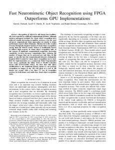
Figure 1: Database consisting of six di�erent airplane silhouettes in standard position. 1’ 1’’ 3’
1’’ 1
2
1
2’’ 1’ 2’
3
2’
3’’ 2’’
2
3 4
Figure 2: A few of the patches stored in the database for an object. Patches i ? i are of length L, as are i0 ? i0 and i00 ? i00. clidean transformation. We choose L such that most patches require 4th degree polynomials for representation. Those few patches requiring greater than 4th degree are smoothed until 4th degree representation is suitable. For simplicity, patches well t by 2nd degree polynomials are squared and patches well t by 3rd degree polynomials are multiplied by the best 1st order t to get the 4th degree representation. We end up with the same number of patches in the raw data and the stored objects. However, a patch on the data may cover a di�erent portion of the object than is covered by any one stored patch. We handle this as follows. In Figure 2 a database object boundary is partitioned into patches
1 ? 1; 2 ? 2; 3 ? 3; etc.. Now in addition, store a second set of patches marked 10 ? 10; 20 ? 20; 30 ? 30 . Patch i0 ? i0 overlaps patch i ? i over 32 of its length. Finally, add a third set of patches 100 ? 100; 200 ? 200; 300 ? 300. The raw data to be recognized is partitioned into a sequence of patches of length 23 L with distance 13 L between adjacent patches. With this representation, it is guaranteed that each patch of length 32 L in the raw data will lie within a patch of length L in the database. The best match will be computed through comparisons of a data patch with all of the patches stored for an object. If there is occlusion in the sensed data, then the number of patches for an object in the data will be di�erent from the number stored for the object in the database. The appropriate matching procedure is to consider patches to be primitives, and then proceed using a recognition tree or indexing based on self or mutual invariants. When the transformations of the data are a�ne, the proper normalization must be used [6]. Recognition involves three additional concepts. 1)Pairs of patches rather than individual patches are recognized (Section 2). 2)Recognition is based on mutual invariants (Section 2). 3)Bayesian recognition is used for mutual invariants (See [5] for Bayesian recognition of self invariants).
2. MUTUAL GEOMETRY AND MUTUAL INVARIANTS We partition the raw data into patches and t a 4th P degree implicit polynomial 0�i+j �4 aij xi yj to each
patch, where a is the coe�cient vector. The polynomial coe�cients of the raw data patches are di�erent from those of the stored objects because of the unknown transformation. Geometric invariants are functions of the coe�cients, that are independent of translations, rotations and di�erent scale changes, but capture polynomial zero set shape information. Hence they can be used in recognizing an object that has undergone an unknown transformation. Recently, invariants of coef cients of polynomials are proving useful in computer vision [1, 2, 3]. Self invariants for each patch provide shape information for the zero set of each polynomial but no information about the position of one polynomial shape with respect to the other because invariants are position invariant. Mutual invariants for a pair of patches capture joint shape information for the pair of polynomials. They provide shape information for individual patches as well as relative position of the two shapes. Pairwise polynomial shape information provides shape information for all of the polynomials jointly. Hence entire object recognition can be accomplished by the
computationally simple procedure of recognizing joint shape geometry for only pairs of polynomials. Let A be the unknown a�ne transformation of the coordinate system. Let � be the coe�cient vector of a polynomial patch in the old coordinate system and �0 be the coe�cient vector of the same polynomial patch in the new transformed system. If a function s(�) satis es s(�0) = jAjw � s(�) where jAj is the determinant of A and w is an integer, then s is called a relative invariant of weight w. If w = 0, then s is an absolute weight invariant. It is called a relative mutual invariant if s is a function of coe�cient vectors of two polynomial patches and satis es the equation. For any implicit polynomial f (x; y), if we multiply its coe�cient vector by a constant nonzero factor c, the resulting implicit polynomial c � f (x; y) has exactly the same zero set as f (x; y) and an invariant should be the same for any such c. If �0 = c � � and s(�0 ) = cd � s(�) where d is a positive integer, then s is called a relative invariant of rank d. If d = 0, then s is an absolute rank invariant. A mutual invariant has rank for each polynomial patch in the pair. Examples of a self and a mutual relative a�ne invariant are the following. Self inv = 6 � a322 ? 27 � a13 � a22 � a31 + 81 � a04 � 2 a31 + 81 � a213 � a40 ? 216 � a04 � a22 � a40 Mutu inv = ?9 � a231 � b04 + 24 � a22 � a40 � b04 + 3 � a22 � a31 � b13 ? 18 � a13 � a40 � b13 ? 2 � a222 � b22 + 3 � a13 � a31 � b22 + 24 � a04 � a40 � b22 + 3 � a13 � a22 � b31 ? 18 � a04 � a31 � b31 ? 9 � a213 � b40 + 24 � a04 � a22 � b40 where a and b are the coe�cient vectors for the two polynomial patches, Self inv has weight 6 and rank 3, Mutu inv has weight 6 and rank 2 in a and rank 1 in b. Using the symbolic computation in [3], we obtained three relative self invariants for each patch and four relative mutual invariants. They are summarized as follows. weight rank a rank b Inv1a 6 4 0 Inv2a 6 3 0 Inv3a 4 3 0 Inv1b 6 0 4 Inv2b 6 0 3 Inv3b 4 0 3 Inv1ab 4 2 1 Inv2ab 4 1 2 Inv3ab 6 2 1 Inv4ab 6 1 2 We construct seven independent rational absolute mutual invariants from these relative invariants. Let Inv = (Inv1a )k1 � (Inv2a )k2 � (Inv3a )k3 � (Inv1b )k4 � (Inv2b)k5 � (Inv3b)k6 � (Inv1ab)k7 � (Inv2ab)k8 � (Inv3ab)k9 � (Inv4ab)k10
(a)
(b)
(c)
Figure 3: (a) Sensed data of an a�ne transformation of plane P1 in the database; (b) its decomposition into patches; (c) polynomial ts to several patches. The coe�cients of the polynomials are used to compute the a�ne mutual invariant vectors. A recognizer is designed based on the Mahalanobis distance between a vector of mutual invariants for a pair of adjacent data patches and that of adjacent template boundary patches in the database. The portion of the polynomial t over the data region is shown darker. where ki; (i = 1; : : :; 10) are integers. Absolute invariants must be weight and rank invariant with regard to a general Euclidean or a�ne transform. weight constraint ) 6k1 + 6k2 + 4k3 + 6k4 + 6k5 + 4k6 + 4k7 + 4k8 + 6k9 + 6k10 = 0 rank constraint in a ) 4k1 +3k2 +3k3 +2k7 + k8 + 2k9 + k10 = 0 rank constraint in b ) 4k4 +3k5 +3k6 + k7 +2k8 + k9 + 2k10 = 0 This yields a linear system with ten variables and three linear constraints. The solution space has dimension 10 ? 3 = 7. Any seven independent solutions will be a basis for this space and generate a set of invariants.
3. EXPERIMENT RESULTS The database in Figure 1 consists of six planes, labeled P1 through P6. Each plane is partitioned into 6 curve patches, each of length L. We store 8 di�erent partition shifts, rather than 3 in Section 1. So for each plane there are 48 curve patches stored, which are obtained by rotating the starting points along the boundary by amounts of 18 L as explained before. The length of raw data patches could then be 78 L and recognition is more accurate. The sensed data to be recognized is shown in Figure 3. It is an a�ne transformation of plane P1 in the data base. The scale changes we have experimented with are 20% or less. Note, the total length of the
Figure 4: Table 1 shows Mahalanobis distance between mutual invariant vector for each pair of adjacent data patches of length 87 L and mutual invariant vector for each pair of adjacent object boundary patches of length L in the database in close to the same position in a plane. Table 2 shows results for plane P1 of comparing each pair of transformed adjacent patches of length 87 L with each pair of stored adjacent patches of length L. plane boundary in the data will be di�erent than that of the plane boundary in the database. We normalize the templates that go into the database and the sensed data such that they t into a square 10x10 box. The normalization can be done because it merely represents an a�ne transformation to which the a�ne invariants used are invariant. Bayesian recognition results are given in Figure 4. An entry in the tables is the Mahalanobis distance between a mutual invariant vector for a pair of adjacent data patches and that of a pair of adjacent template boundary patches in the database. The Mahalanobis distance has the form (GMN ? G^ ij )t ij (GMN ? G^ ij ) where G^ ij is the vector of mutual invariants for the two polynomials t to the ith and j th patches in the data, ij is a weighting matrix based on the ith and j th data patches to be recognized, and GMN is the vector of mutual invariants for the two polynomials t to the M th and N th patches of a plane in the database. Of great importance is that the Bayesian recognizer permits comparison of invariants of patches of length L in the database with subpatches of length 87 L (or somewhat smaller) in the measured data [6]. In Table 1 of Figure 4, mutual invariants for pairs of patches in the data are being compared with pairs of patches in roughly the same positions on each plane in the database, thus resulting in a worst recognition situation for false alarms. For example, column 2 ? 3 is the Mahalanobis distance between the measured mutual in-
Figure 5: Sensed data of an a�ne transformation for an animal in the database, its decomposition into patches, and polynomial ts to several patches. variants vector for patches 2 and 3 in Figure 3 with the mutual invariants vector in the database in close to the same position for each of the six planes. Since the measurements are for a transformed version of P1, the entree in row P1 should be the smallest. Note, this is the case almost everywhere in the table except for a few entrees in columns 3 ? 4 and 5 ? 6. Among the reasons for this problem is that patch 5 ends in a high curvature region. A number of implementation issues are discussed in [6]. In Table 2, mutual invariants for each pair of patches in the data is compared with each pair of patches stored for plane P1. Hence each diagonal element is the comparison of a pair of sensed data patches of P1 with a pair stored for P1 with roughly the same position. The diagonal elements in second table are the same as those row elements for plane P1 in rst table. And the wrong pairwise matches will usually generate big errors. Figure 5 is an example of application to shapes that are free-form. In Figure 6 nearly half of the plane has been occluded and two boundary patches of the occluding surface have been attached to the plane boundary. We have seven patches for the sensed data set. But patches from the occluding boundary will have big distances no matter which stored invariant vector they are compared with. So they should be rejected as unrecognizable [6]. The patches from the true object boundary still match those corresponding patches in the database well.
Acknowledgements This work was partially supported by NSF Grant #IRI-9224963.
Figure 6: The sensed data is a partially occluded, transformed version (with less than 5% scaling) of database plane P2. 4.
REFERENCES
[1] J.L. Mundy and A. Zisserman. editors, Geometric Invariance in Computer Vision, MIT Press, 1992 [2] G. Taubin. Estimation of planar curves, surfaces and nonplanar space curves de ned by implicit equations, with applications to edge and range image segmentation. IEEE Transactions on Pattern Analysis and Machine Intelligence, November 1991. [3] D. Keren. Some New Invariants in Computer Vision. IEEE Transactions on Pattern Analysis and Machine Intelligence. November 1994. [4] M. Barzohar, D. Keren and D.B. Cooper. Recognizing Groups of Curves Based on New A�ne Mutual Geometric Invariants, with Applications to Recognizing Intersecting Roads in Aerial Images. In Proceedings of 12th International Conference on Pattern Recognition, Jerusalem, Israel, October 1994. [5] J. Subrahmonia, D. Keren, and D.B. Cooper. An Integrated Object Recognition System Based on High Degree Implicit Polynomials, Algebraic Invariants, and Bayesian Methods. In Proceedings: ARPA Image Understanding Workshop, DC, April 1993. [6] Z. Lei, D. Keren and D.B. Cooper. Recognition of Complex Free-Form Objects Based on Mutual Algebraic Invariants for Pairs of Patches of Data. Lems report 140, Division of Engineering, Brown University, January 1995.