Vol. 17, No. 5-6, May – June 2015, p. 877 - 883
JOURNAL OF OPTOELECTRONICS AND ADVANCED MATERIALS
Computing topological polynomials of certain nanostructures A. Q. BAIGa*, M. IMRANb, H. ALIa, S. U. REHMANa a Department of Mathematics, COMSATS Institute of Information Technology, Attock, Pakistan b Department of Mathematics, School of Natural Sciences (SNS), National University of Sciences and Technology (NUST), Sector H-12, Islamabad, Pakistan
Counting polynomials are those polynomials having at exponent the extent of a property partition and coefficients the multiplicity/occurrence of the corresponding partition. In this paper, Omega, Sadhana and PI polynomials are computed for Multilayer Hex-Cells nanotubes, One Pentagonal Carbon nanocones and Melem Chain nanotubes. These polynomials were proposed on the ground of quasi-orthogonal cuts edge strips in polycyclic graphs. These counting polynomials are useful in the topological description of bipartite structures as well as in counting some single number descriptors, i.e. topological indices. These polynomials count equidistant and non-equidistant edges in graphs. In this paper, analytical closed formulas of these polynomials for Multi-layer Hex-Cells MLH (k, d) nanotubes, One Pentagonal Carbon CNC5 (n) nanocones and Melem Chain MC (n) nanotubes are derived. (Received March 2, 2015; accepted May 7, 2015) Keywords: Counting polynomial, Omega polynomial, Sadhana polynomial, PI polynomial, MLH (k, d) nanotubes, CNC5 (n) nanocones, MC (n) nanotubes
P(G) = P(G, x) |x =1 = m(G, k ) k
1. Introduction and preliminary results Mathematical chemistry is a branch of theoretical chemistry in which we discuss and predict the chemical structure by using mathematical tools and doesn’t necessarily refer to the quantum mechanics. Chemical graph theory is a branch of mathematical chemistry in which we apply tools from graph theory to model the chemical phenomenon mathematically. This theory contributes a prominent role in the fields of chemical sciences. Carbon nanotubes (CNTs) are types of nanostructure which are allotropes of carbon and having a cylindrical shape. Carbon nanotubes, a type of fullerene, have potential in fields such as nanotechnology, electronics, optics, materials science, and architecture. Carbon nanotubes provide a certain potential for metal-free catalysis of inorganic and organic reactions. Counting polynomials are those polynomials having at exponent the extent of a property partition and coefficients the multiplicity/occurrence of the corresponding partition. A counting polynomial is defined as:
P(G, x) = m(G, k ) x
k
(1)
k
Where the coefficient m(G, k ) are calculable by various methods, techniques and algorithms. The expression (1) was found independently by Sachs, Harary, Mili c , Spialter, Hosoya, etc [5]. The corresponding topological index P(G) is defined in this way:
k
A moleculer/chemical graph is a simple finite graph in which vertices denote the atoms and edges denote the chemical bonds in underlying chemical structure. This is more important to say that the hydrogen atoms are often omitted in any molecular graph. A graph can be represented by a matrix, a sequence, a polynomial and a numeric number (often called a topological index) which represents the whole graph and these representations are aimed to be uniquely defined for that graph. Two edges e = uv and f = xy in E (G) are said to be codistant, usually denoted by
e co f , if
d ( x, u) = d ( y, v) and
d ( x, v) = d ( y, u) = d ( x, u) 1 = d ( y, v) 1
The relation “ co " is reflexive as all edges in G , also symmetric as if
e co e is true for e co f then f co e for all e, f E (G) but the relation “ co " is not
necessarily transitive. Consider
C(e) = { f E(G) : f co e} If the relation is transitive on C (e) also, then C (e) is called an orthogonal cut “ co " of the graph
G . Let
878
A. Q. Baig, M. Imran, H. Ali, S. U. Rehman
e = uv and f = xy be two edges of a graph G , which are opposite or topological parallel, and this relation is denoted by e op f . A set of opposite edges, within the same face or ring, eventually forming a strip of adjacent faces/rings, is called an opposite edge strip ops, which is a quasi-orthogonal cut qoc (i.e. the transitivity relation is not necessarily obeyed). Note that “ co " relation is defined in the whole graph while “ op " is defined only in a face/ring.
Ashrafi et al. computed Sadhana polynomial of V-phenylenic nanotube and nanotori. Theorem 1.0.2. [1] Let G be the graph of V-phenylenic nanotube, then Sadhana polynomial of
G is
Max{m , n}1
Sd (G, x) = 4
x|E (G )| 2i 2(| n m | 1) x|E (G )| 2 Min{m,n}
i =1
In this article, G is considered to be simple connected graph with vertex set V (G) and edge set
nx|E (G )|2m (m 1) x|E (G )|2m (n 1) x|E (G )| n
E (G) , m(G, k ) be the number of ops of length k , e =| E (G) | is the edge cardinality of G .
All nanotubes are allotropes of carbon and are a type of fullerene. Ghorbani et al. computed Omega and Sadhana
The omega polynomial was introduced by Diudea et al. in 2006 on the ground of op strips. The Omega polynomial is proposed to describe cycle-containing molecular structures, particularly those associated with nanostructures. Definition 1.1. [6] Let G be a graph, then its Omega polynomial denoted by (G, x) in x is defined as
(G, x) = m(G, k ) x
polynomials of an infinite family of fullerene
n 10 . Theorem 1.0.3. [11] Consider the fullerene graph
C10n , n 10 . Then the Omega and Sadhana polynomials of C10n are computed as follows: (C10n , x)
k
k
Sd (G, x) = m(G, k ) x
n 2
3
n 3 2
5x
5x
n 3 2
10 x n3 2 ∤ 𝑛
Sd (C10n , x) 15n 3
10 x
10 x
15n 3 5x { 10 x
ek
3
10 x 10 x 10 x n3 0.35cm 2 | n { 10 x
The Sadhana polynomial is defined based on counting opposite edge strips in any graph. This polynomial counts equidistant edges in G . Definition 1.2. [8] Let G be a graph, then Sadhana polynomial denoted by Sd (G, x) is defined as
C10n ,
29n 2
29n 3 2
10 x14n3 0.35cm 2 | n
5x
29n 3 2
10 x14n3 , 2 ∤ 𝑛
k
The PI polynomial is also defined based on counting opposite edge strips in any graph. This polynomial counts non-equidistant edges in G . Definition 1.3. [8] Let G be a graph, then PI polynomial denoted by PI (G, x) is defined as
2. Results and Discussion
PI (G, x) = m(G, k ) k x ek k
Yazdani et al. determined Padmakar-Ivan (PI) polynomials
HAC5C6C7 [4 p,2q]
of
nanotubes.
G be the HAC5C6C7 nanotube, then PI polynomial of G is Theorem 1.0.1. [21] Let
PI (G, x) = qx
9 pq
p 4
px
9 pq
p 6q 4
4qx
(|𝑉(𝐺)|+1 ) 2
3 2 7 where | V (G ) |= p q q p 2 2
9 pq
15 p2 4
The preceding results are used to compute their corresponding topological indices which provides a good model correlating the certain physico-chemical properties of these carbon allotropes.
9 pq
p 4
In this paper, we compute Omega, Sadhana and PI polynomials for Multilayer Hex-Cells MLH (k, d) nanotubes, One Pentagonal Carbon CNC5 (n) nanocones and Melem Chain MC (n) nanotubes. For further study of these polynomials their topological indices and polynomials of various nanotubes, consult [3, 4, 7, 10, 12-18, 20]. These polynomials are used to predict various physico-chemical properties of certain chemical compounds. 2.1. Multilayer Hex-Cells MLH (k, d) nanotubes In this section, we compute Omega, Sadhana and PI polynomials for MLH (k, d) nanotubes. A Hex-Cell nanotube [19] with depth d is denoted by HC (d) and can be constructed by using units of hexagon cells, each of six
Computing topological polynomials of certain nanostructures
vertices. A Hex-Cell nanotube with depth d has d levels numbered from 1 to d, where level 1 represents the innermost level corresponding to one hexagon cell. Level 2 corresponds to the six hexagon cells surrounding the hexagon at level 1. Level 3 corresponds to the 12 hexagon cells surrounding the six hexagons at level 2 as shown in Figure 1. Each level i has Vi vertices, where Vi = 6(2i - 1) and the total number of vertices in a Hex-Cell nanotubes HC (d) is V = 6d2. The Multilayer Hex-Cell (MLH) is a modular interconnection network that consists of layers of identical Hex-Cells nanotubes connected together in hierarchical fashion as shown in Figure 2. The MLH is denoted by MLH (k, d), where k denotes the layer number, and d denotes the depth of the identical Hex-Cell. This family of nanotubes is usually symbolized as MLH (k, d). We have |V (MLH (k, d))| = 6kd2 and |E (MLH (k, d))| =
879
Proof: Let G be the graph of MLH (k, d) nanotubes ∀ k, d ∈ ℕ. Table 1 shows the number of co-distant edges in G. By using table 1 the proof is mechanical.
k 1
6(2k +
2(k + r)) + 6kd . 2
r =1
Fig. 2. MLH (2, 2).
Table 1. Number of co-distant edges of MLH (k,d) nanotube. Types of Types of qoc’s edges
No of co-distant edges k 1
e1
C1
No of qoc
2k 2(k r )
k 1
2k 1 2(2k r 1) r =1
r =1
C2
k 1
k 1
2k 2(k r )
e2
2k 1 2(2k r 1)
r =1
C3
Fig. 1. (a) HC (one level) (b) (two levels) (c) (three levels).
r =1
k 1
e3
2k 2(k r )
k 1
2k 1 2(2k r 1) r =1
r =1
C4
Theorem 2.1.1. The Omega polynomial of MLH (k, d) nanotubes ∀ k, d ∈ ℕ, is as follows: Ω 𝑀𝐿𝐻(𝑘, 𝑑) = 6((2𝑘 − 1)
+2
(2k − r − 1)x
2(2k+
6kd2
k-1
Now we apply formula and do some calculation to get our result.
k 1
k 1
e4
2(k+r))
r =1
r =1 2
+ (k − 1)x 6kd ).
(G, x) = m(G, k ) x k k k 1
k 1
(G, x) = 2(2k 1) 2(2k r 1) x
2(2 k
k 1
2(k r ))
r =1
k 1
2(2k 1) 2(2k r 1) x
r =1
2(2 k
2(k r ))
r =1
r =1
k 1
k 1
2(2k 1) 2(2k r 1) x
2(2 k
2(k r ))
r =1
(k 1) x 6 kd
2
r =1
k 1
k 1
(G, x) = 6((2k 1) 2(2k r 1) x r =1
Now
we
compute
Sadhana
polynomial
of
2(2 k
r =1
2(k r )) 2
(k 1) x 6 kd )
MLH (k , d ) nanotube k, d ∈ ℕ. Following theorem
880
A. Q. Baig, M. Imran, H. Ali, S. U. Rehman
shows the Sadhana polynomial for this family of nanotubes. Theorem 2.1.2. Consider the graph of MLH (k , d )
k, d ∈ ℕ. Then its Sadhana polynomial is as
nanotube follows:
k 1
k 1
Sd ( MLH (k , d ), x) = 6((2k 1) 2(2k r 1)) x
4(2 k
k 1
2(k r ) k 6 d 2 )
6(2 k
(k 1) x
r =1
2(k r ))
r =1
r =1
that G be the graph of MLH (k , d ) nanotube k, d ∈ ℕ. The proof of this result is just calculation based. We prove it by using table 1 . We know Sd (G, x) = m(G, k ) x ek Proof. Let
k
k 1
k 1
Sd (G, x) = 2((2k 1) 2(2k r 1)) x
6(2 k
k 1
2(k r ) 6 kd 2 ) 2(2 k
r =1
2(k r ))
r =1
r =1 k 1
k 1
2((2k 1) 2(2k r 1)) x
6(2 k
k 1
2(k r ) 6 kd 2 ) 2(2 k
r =1
2(k r ))
2((2k 1)
r =1
r =1 k 1
k 1
2(2k r 1)) x
6(2 k
k 1
2(k r ) 6 kd 2 ) 2(2 k
r =1
k 1
2(k r ))
6(2 k
(k 1) x
r =1
2(k r )) 6 kd 2 6 kd 2
r =1
r =1
k 1
k 1
Sd (G, x) = 6((2k 1) 2(2k r 1)) x
4(2 k
6(2 k
(k 1) x
r =1
r =1
Next we compute PI polynomial of MLH (k , d ) nanotube. Following theorem explains the PI polynomial of this family of nanotubes. Theorem 2.1.3. Consider the graph of MLH (k , d )
k 1
2(k r ) k 6 d 2 )
nanotube follows:
2(k r ))
r =1
k, d ∈ ℕ. Then its PI polynomial is as
k 1
k 1
r =1
r =1
PI ( MLH (k , d ), x) = 12(2k (2k 1) (2k 1)2(k r ) 4k (2k r 1) k 1
k 1
k 1
2(2k r 1)(2(k r ))) x r =1
Proof. Let
4(2 k
k 1
2(k r )) 6 kd 2
r =1
k 1
2(k 1)(2k 2(k r )) x
r =1
6(2 k
2(k r ))
r =1
r =1
k, d ∈ ℕ. We prove it by using table 1. We know that G be the graph of MLH (k , d ) nanotube PI (G, x) = m(G, k ) k x ek k k 1
k 1
k 1
PI (G, x) = 2((2k 1) 2(2k r 1)) 2(2k 2(k r ) x r =1
6(2 k
k 1
2(k r )) 6 kd 2 2(2 k
r =1
2(k r ))
r =1
r =1 k 1
k 1
k 1
r =1
r =1
2((2k 1) 2(2k r 1)) 2(2k 2(k r ) x
6(2 k
r =1
k 1
2(k r )) 6 kd 2 2(2 k
r =1
2(k r ))
Computing topological polynomials of certain nanostructures
881
k 1
k 1
k 1
2((2k 1) 2(2k r 1)) 2(2k 2(k r ) x r =1
6(2 k
k 1
2(k r )) 6 kd 2 2(2 k
r =1
2(k r ))
r =1
r =1 k 1
k 1
2(k 1)(2k 2(k r )) x
6(2k
2(k r )) 6 kd 2 6 kd 2
r =1
r =1
k 1
k 1
r =1
r =1
PI (G, x) = 12(2k (2k 1) (2k 1)2(k r ) 4k (2k r 1) k 1
k 1
k 1
2(2k r 1)(2(k r ))) x r =1
4(2 k
k 1
2(k r )) 6 kd 2
r =1
2(k 1)(2k 2(k r )) x
r =1
2.2 One pentagonal carbon
CNC5 (n)
for
n3
In this section, we determine Omega, Sadhana and PI
CNC5 (n) , n 3 nanocones. One
pentagonal carbon nanocones, Fig. 3, originally discovered by Ge and Sattler in 1994 [9]. These are constructed from
CNC5 (n)
and edges are 5n
2
G be the graph of one pentagonal carbon CNC5 (n) for n 3 nanocone. Table 2 shows the number of co-distant edges in G . By using table 2 , the proof is straightforward. Table 2. Number of co-distant edges of
n3
nanocone, the number of vertices
Types Types of qoc of edges
5 n(3n 1) respectively. 2
C1 C2
and
2(k r ))
r =1
Proof. Let
o
a graphene sheet by removing a 60 wedge and joining the edges produces a cone with a single pentagonal defect at the apex. In
r =1
nanocones
polynomials for
k 1
6(2 k
CNC5 (n)
nanocone.
No. of co-distant edges
n
e1 e2
for
No. of qoc
5 5
n2
(n i) i =1
C3
2n 1
e3
5
Now we apply formula and do some easy calculation to get our result.
(G, x) = m(G, k ) x k k
n2
(G, x) = 5 x 5 x n
i =1
( n i )
5 x 2 n 1
n2
( ni )
(G, x) = 5 x Fig. 3. A representation of
CNC5 (7)
Now we compute Omega polynomial of nanocone. Theorem
CNC5 (n)
2.2.1.
The
nanocone for
Omega
nanocone. n2
CNC5 (n)
polynomial
n 3 is as follows:
(CNC5 (n), x) = 5( x
( ni )
(G, x) = 5( x
i =1
x n ( x n 1 1))
In the following theorem, the Sadhana polynomial of Theorem 2.2.2. The Sadhana polynomial of one
( n i )
i =1
of
CNC5 (n) for n 3 nanocone is computed.
n2
5 x n ( x n 1 1)
i =1
x (x n
n 1
1))
pentagonal carbon
CNC5 (n) for n 3 nanocone is as
882
A. Q. Baig, M. Imran, H. Ali, S. U. Rehman
follows: n2
Sd (CNC5 (n), x) = 5( x
n (15n 7) 2
G be the graph of one pentagonal carbon CNC5 (n) for n 3 nanocone. By using table 2 the Proof. Let
proof is easy. Now we apply formula and do some computation to get our result.
x
5 n (3 n 1) 2
( n i )
3
x2
i =1
( n (5 n 3)1)
o
respectively) at temperatures up to 450 C in sealed glass ampules. The vertices and edges in Melem chain are 18n 4 and 21n 3 respectively. Now we compute Omega polynomial of melem chain MC (n) nanotube.
n2
Sd (G, x) = 5 x
5 n (3 n 1) n 2
5x
5 n (3 n 1) 2
( n i )
5
5x 2
i =1
n (3 n 1)(2 n 1)
n2
5( x
n (15n 7) 2
x
5 n (3 n 1) 2
( n i )
i =1
3
x2
( n (5 n 3)1)
PI polynomial of one pentagonal carbon for
CNC5 (n)
n 3 nanocone is computed in [2]. Fig. 4. A representation of
2.3 Melem chain MC (n) for
n∈ℕ
In this section, we compute Omega, Sadhana and PI polynomials for melem
nanotube.
Theorem 2.3.1. The Omega polynomial of nanotube MC (n) for n ∈ ℕ is equal to:
(2,5,8 triamino tri s triazine)
(MC(n), x) = (6n 5) x 7 n1
C6 N7 (NH 2 )3 chain nanotube. Melem was obtained as a crystalline powder by thermal treatment of different less condensed C N H compounds (e.g., melamine
C3 N3 (NH 2 )3 ,
MC (4)
dicyandiamide H 4C2 N 4 , ammonium
G be the graph of MC (n) nanotube for n ∈ ℕ. Table 3 shows the number of co-distant edges in G . By using table 3 the proof is straightforward. Proof. Let
dicyanamide NH 4 [ N (CN ) 2 ] , or cyanamide H 2CN 2 , Table 3. Number of co-distant edges of
Types of qoc
Types of edges
C1 C2
e1 e2
C3
e3
(G, x) = (3n 1) x
k 7 n 1
(3n 1) x7 n1 3x 7 n1
(G, x) = (3n 1 3n 1 3) x 7 n1 (G, x) = (6n 5) x7 n1
nanotube.
No. of co-distant edges
Now we apply formula and do some easy calculation to get our result.
(G, x) = m(G, k ) x k
MC (n)
7n 1 7n 1 7n 1
No. of qoc
3n 1 3n 1 3
In the following theorem, the Sadhana polynomial of
MC (n) nanotube is computed. Theorem 2.3.2. The Sadhana polynomial of MC (n) nanotube for
n ∈ ℕ is as follows:
Sd (, x) = (6n 5) 2(7n1) Proof. Let G be the graph MC (n) nanotube for n ∈ ℕ. By using table 3 the proof is easy. Now we apply formula and do some computation to get our result.
Computing topological polynomials of certain nanostructures
883
Sd (G, x) = m(G, k ) x ek k
Sd (G, x) = (3n 1) x
21n 3(7 n 1)
(3n 1) x 21n3(7 n1) 3x 21n3(7 n1)
Sd (G, x) = (3n 1) x 21n37 n1 (3n 1) x 21n37 n1 3x 21n37 n1 Sd (, x) = (6n 5) 2(7n1) Now we compute PI polynomial of
PI (G, x) = (42n2 41n 5) x 2(7n1)
MC (n)
nanotube for n ∈ ℕ. Following theorem shows the PI polynomial for this finite family of nanotubes. Theorem 2.3.3. Consider the graph of MC (n) nanotube for
Proof. Let
G be the graph of MC (n) nanotube for
n ∈ ℕ. The proof of this result is just calculation based. We easily prove it by using table 3 . We know that
n ∈ ℕ. Then its PI polynomial is as follows:
PI (G, x) = m(G, k ) x ek k
21n 3(7 n 1)
PI (G, x) = (3n 1)(7n 1) x (3n 1)(7n 1) x 21n3(7 n1) 3(7n 1) x 21n3(7 n1) PI (G, x) = (21n2 10n 1) x 21n37 n1 (21n2 10n 1) x 21n37 n1 (21n 3) x 21n37 n1 PI (, x) = (42n2 41n 5) x 2(7n1) 3. Conclusion and general remarks In this paper, three important counting polynomials called Omega, Sadhana and PI are studied. These polynomials are useful in determining Omega, Sadhana and PI topological indices which play an important role in QSAR/QSPR study. We computed these polynomials for
MLH (k , d ) nanotube, CNC5 (n) MC (n) nanotube.
nanocone
and
References [1] A. R. Ashrafi, M. Ghorbani, M. Jalali, Indian J. Chem., 47A, 535 (2008).. [2] A. R. Ashrafi, H. Saati, J. Comput. Theor. Nanosci. 4, 1 (2007). [3] A. Bahrami, J. Yazdani, Digest Journal of Nanomaterials and Biostructures, 3, 265 (2008). [4] A. Q. Baig, M. Imran, H. Ali, Computing Omega, Optoelectron. Adv. Mater. –Rapid Commun, 6, 248 (2015). [5] K. C. Das, F. M. Bhatti, S. G. Lee, I. Gutman, MATCH Commun. Math. Comput. Chem. 65, 753 (2011). [6] M. V. Diudea, Carpath. J. Math., 22, 43 (2006). [7] M. V. Diudea, S. Cigher, P. E. John, MATCH Commun. Math. Comput. Chem. 60, 237 (2008). [8] M. V. Diudea, I. Gutman, J. Lorentz, Molecular Topology, Nova, Huntington 2001. [9] M. Ge, K. Sattler, Chem. Phys. Lett. 220(192), 2284 (1994).
[10] M. Ghojavand, A. R. Ashrafi, Digest Journal of Nanomaterials and Biostructures 3, 209 (2008).. [11] M. Ghorbani, M. Jalali, Digest Journal of Nanomaterials and Biostructures, 4, 177 (2009). [12] S. Hayat, M. Imran, Studia UBB Chemia, 59(4), 113(2014). [13] S. Hayat, M. Imran, J. Comput. Theor. Nanosci., 12, 70(2015) [14] S. Hayat, M. Imran, J. Comput. Theor. Nanosci., 12, 533(2015). [15] S. Hayat, M. Imran, J. Comput. Theor. Nanosci., Accepted, In press. [16] M. Imran, S. Hayat, M. K. Shafiq, Optoelectron. Adv. Mater. - Rapid Commun. 8(9-10), 948 (2014). [17] M. Imran, S. Hayat, M. K. Shafiq, Optoelectron. Adv. Mater. - Rapid Commun., 8(11-12), 1218 (2014). [18] B. Rajan, A. William, C. Grigorious, S. Stephen, J. Comp. Math. Sci., 5, 530 (2012). [19] A. Sharieh, M. Qatawaneh, W. Almobaideen, A. Sliet, Hex-Cell, Euoropian journal of Scientific Research 22, 457 (2008). [20] I. Tomescu, S. Kanwal, MATCH Commun. Math. Comput. Chem., 69, 535 (2013).. [21] J. Yazdani, A. Bahrami, Digest Journal of Nanomaterials and Biostructures, 4, 507 (2009).
_____________________________ * Corresponding author:
[email protected]