3.10 Block diagram of the end-effector with applied damping in intrinsic con- figuration . ... 4.14 Non-unique solution for actuator and spring coordinates for gait cycle . . 38. 4.15 Non-unique .... means that the end-effector is connected to the base by more than one independent kine- ...... approximate mass of 63 kg. Table 4: ...
University of Liège
Faculty of Applied Science
Conceptual Design of a Variable Stiffness Mechanism using Parallel Redundant Actuation Academic Year 2017 - 2018
Author:
Christoph Stoeffler
1st examiner:
Prof. Dr. Olivier Brüls
University of Liège
2nd examiner:
Prof. Dr. Frank Kirchner
University of Bremen
1st supervisor:
Shivesh Kumar
DFKI Bremen - Robotics Innovation Center
2nd supervisor:
Heiner Peters
DFKI Bremen - Robotics Innovation Center
Graduation Studies conducted for obtaining the Master’s degree in “Aerospace Engineering” by Christoph Stoeffler.
Contents Symbols and Abbreviations
vi
Abstract
vii
Acknowledgements
1
1 Introduction
2
2 The 2.1 2.2 2.3
Variable Stiffness Mechanism - An Parallel Mechanisms . . . . . . . . . . Variable Impedance Actuators . . . . . Variable Stiffness Mechanism . . . . .
Overview . . . . . . . . . . . . . . . . . . . . . . . . . . . . . . . . . . . . . . . . . . . . . . . . . . . . . . . . .
3 Modelling of the Mechanism 3.1 Mobility of the Non-Redundant and Redundant Mechanism 3.2 Inverse Kinematics . . . . . . . . . . . . . . . . . . . . . . . 3.3 Differential Kinematics . . . . . . . . . . . . . . . . . . . . . 3.3.1 Jacobian Matrix for Redundant Actuation . . . . . . 3.4 Pneumatic Spring Model . . . . . . . . . . . . . . . . . . . . 3.5 Stiffness Model . . . . . . . . . . . . . . . . . . . . . . . . . 3.6 Quasi-static Model . . . . . . . . . . . . . . . . . . . . . . . 3.7 Dynamic Model in OpenModelica . . . . . . . . . . . . . . .
4 4 6 8
. . . . . . . .
10 11 12 14 16 18 20 22 24
. . . . . . .
27 27 29 31 33 35 37 40
5 Design of a Test Environment 5.1 Actuation Leg . . . . . . . . . . . . . . . . . . . . . . . . . . . . . . . . .
46 47
6 Conclusion and Outlook
50
References
56
4 Simulation and Results 4.1 Design Parameters . . . . . . . . . . . . . . . . . 4.2 Singularity and Dexterity for Rigid Design . . . . 4.3 Velocity and Force Transmission for Rigid Design 4.4 End-effector Stiffness . . . . . . . . . . . . . . . . 4.5 Quasi-static computations . . . . . . . . . . . . . 4.6 Simulation of Human Gait . . . . . . . . . . . . . 4.7 Comparison with OpenModelica . . . . . . . . . .
i
. . . . . . .
. . . . . . .
. . . . . . .
. . . . . . .
. . . . . . .
. . . . . . .
. . . . . . . .
. . . . . . .
. . . . . . . .
. . . . . . .
. . . . . . . .
. . . . . . .
. . . . . . . .
. . . . . . .
. . . . . . . .
. . . . . . .
. . . . . . . .
. . . . . . .
APPENDIX A - Results under Extrinsic Rotation
58
APPENDIX B - Simulation Algorithms
60
APPENDIX C - Testbed Design Data
62
APPENDIX D - Back Computation of Gait Cycle
63
ii
List of Figures 2.1 2.2
Basic conceptual idea of a variable stiffness mechanism . . . . . . . . . . Left: Leg mechanism composed of ten joints, right: Scheme of running wooden horse. Source: [51] . . . . . . . . . . . . . . . . . . . . . . . . . . 2.3 Principle of the VIA developed at the German Aerospace Center . . . . . 2.4 Working principle of the antagonistic (left) and serial (right) VIA. Figure according to [9] . . . . . . . . . . . . . . . . . . . . . . . . . . . . . . . . 2.5 Humanoids JUSTIN (left) and DAVID (right) performed as simulated compliant and intrinsically compliant robots. Source: www.dlr.de . . . . . . . 2.6 Left: Four-bar mechanism performed as rigid mechanism. Right: Flexibleredundant mechanism (VSM). . . . . . . . . . . . . . . . . . . . . . . . . 3.1 Overview of the created models . . . . . . . . . . . . . . . . . . . . . . . 3.2 Extension of a parallel mechanism to the proposed concept . . . . . . . . 3.3 Overview of the redundant ankle mechanism with particular motion manifold 3.4 Overview of the redundant ankle mechanism with flexible elements . . . 3.5 Rigid body transformations coming from actuator and spring . . . . . . . 3.6 Mapping of 3D actuation space to 2D workspace . . . . . . . . . . . . . . 3.7 Double-acting pneumatic cylinder with equal volumes . . . . . . . . . . . 3.8 Unit spring force of the closed pneumatic cylinder over normalized passive coordinate . . . . . . . . . . . . . . . . . . . . . . . . . . . . . . . . . . . 3.9 Depiction of model components in OMEdit representing one leg of the VSM. . . . . . . . . . . . . . . . . . . . . . . . . . . . . . . . . . . . . . 3.10 Block diagram of the end-effector with applied damping in intrinsic configuration . . . . . . . . . . . . . . . . . . . . . . . . . . . . . . . . . . . 4.1 Plot of the geometry in zero configuration inside numerical simulation. green: upper attachment structure, black: structure from {s}-frame to {b}-frame, red: lower attachment structure and blue: actuation legs . . . 4.2 Four main movements in the human ankle. Source: [11] . . . . . . . . . . 4.3 Comparison of manipulability and dexterity for the non-redundant and redundant design . . . . . . . . . . . . . . . . . . . . . . . . . . . . . . . 4.4 Actuator force and speed for pure roll movement when end-effector force and speed are given . . . . . . . . . . . . . . . . . . . . . . . . . . . . . . 4.5 Actuator force and speed for pure pitch movement when end-effector force and speed are given . . . . . . . . . . . . . . . . . . . . . . . . . . . . . . 4.6 Power of all three actuators under pure roll movement when end-effector force and speed are given . . . . . . . . . . . . . . . . . . . . . . . . . . .
iii
4 5 6 7 7 9 10 11 13 14 15 17 18 19 24 25
28 29 30 31 32 33
4.7 4.8 4.9 4.10 4.11 4.12 4.13 4.14 4.15 4.16 4.17 4.18 4.19 4.20 4.21 4.22 5.1 5.2 5.3
Power of all three actuators under pure pitch movement when end-effector force and speed are given . . . . . . . . . . . . . . . . . . . . . . . . . . . Stiffness changes for pure roll and pure pitch . . . . . . . . . . . . . . . . Roll and pitch stiffness over the complete work range . . . . . . . . . . . Stiffness, position and force changes by front actuator variation . . . . . Stiffness, position and force changes by front and one rear actuator variations Stiffness, position and force changes by three simultaneous actuator variations . . . . . . . . . . . . . . . . . . . . . . . . . . . . . . . . . . . . . Resulting ankle torque and angle. Interpolation data according to [20] . . Non-unique solution for actuator and spring coordinates for gait cycle . . Non-unique solution for actuator and spring coordinates for gait cycle with front spring restricted to 50 % deflection . . . . . . . . . . . . . . . . . . Unique solution for gait cycle under predefined stiffness . . . . . . . . . . Error in roll and pitch angle for three different load cases . . . . . . . . . Error in actuator forces for three different load cases . . . . . . . . . . . Stiffness curves arising from changes in da1 . . . . . . . . . . . . . . . . . Stiffness curves arising from changes in da1 and da2 . . . . . . . . . . . . . Stiffness curves arising from changes in da1 , da2 and da2 . . . . . . . . . . . Error between rigid actuator lengths in OpenModelica and the quasi-static computations . . . . . . . . . . . . . . . . . . . . . . . . . . . . . . . . . Design of a variable test environment . . . . . . . . . . . . . . . . . . . . One actuation leg of the VSM with pneumatic element . . . . . . . . . . View of the end-effector of the system with mounted inductive sensors for the rotatory DOFs . . . . . . . . . . . . . . . . . . . . . . . . . . . . . .
iv
33 34 35 36 36 37 38 38 39 39 40 41 42 43 43 44 46 47 48
List of Tables 1 2 3 4
Advantages and drawbacks of PRMs compared to SMs . . . . . . . . . . 6 Overview of the different quasi-static functions - the number of output variables also defines the number of necessary equations inside the functions. 22 Averaged ankle data from [17],[12], [32], [3] and [41]. . . . . . . . . . . . . 29 Design data of the actuators in rigid configuration . . . . . . . . . . . . . 32
v
Symbols and Abbreviations
~bi c0 d~i df0 f g H J Jq Jx J† K m ~s M Mnr p0 p1 qa qf Rsb ~si ~u x xc β γ κ τ
spatial vector of attachment point in {b}-frame pneumatic constant of the pneumatic spring spatial vector of one actuation leg maximal piston stroke of pneumatic spring forces in tasks-space vector of kinematic constraints Hessian matrix of the constraints Jacobian matrix of the constraints partial, actuation space dependent Jacobian matrix of the constraints partial, work space dependent Jacobian matrix of the constraints Moore-Penrose pseudo-inverse of Jacobian matrix stiffness matrix of end-effector torques in {s}-frame mobility after Grübler-criterion mobility for non-redundant mechanism initial pressure of pneumatic spring pressure in state 1 of pneumatic spring vector of actuator coordinates vector of spring coordinates rotation matrix between {b}-frame and {s}-frame spatial vector of attachment point in {s}-frame spatial vector pointing from {b}-frame to {s}-frame vector of end-effector coordinates configuration specific vector of end-effector coordinates pitch angle of end-effector roll angle of end-effector heat-capacity ratio vector of actuation forces
DFKI Deutsches Forschungszentrum für Künstliche Intelligenz DOF Degrees of Freedom ODE Ordinary Differential Equation PDE Partial Differential Equation PM Parallel Mechanism PRM Parallel Redundant Mechanism SM Serial Mechanism SVD Singular Value Decomposition VIA Variable Impedance Actuator VSM Variable Stiffness Mechanism
vi
Abstract Future robots will rely more than today on high precision, better energy efficiency and safe handling (e.g. human-machine interaction). An inevitable step in the development of new robots is therefore the improvement of existing mechanisms, since better sensors and algorithms do not satisfy the demands alone. During the last three decades Parallel Redundant Mechanisms (PRM) came more in the focus of research, as they are advantageous in terms of singularity avoidance, fast movements and energy efficiency. Subsequently, yet another technology - the Variable Impedance Actuator (VIA) - emerged which proposes to change its inherent properties allowing an adaption to its environment and to handle for example dynamic movements or shock absorptions. This work aims to create a new mechanism where a stiffness and position control for 2 degrees of freedom (DOF) is achieved with 3 actuators. It is thus a combination of the PRM and VIA, while taking advantage of both technologies but asking for a more sophisticated mathematical description. Practical implementation is intended for a humanoid ankle mechanism. Kinematic, quasi-static and stiffness models are derived and incorporated for the simulation of the mechanism and compared to a dynamic model in OpenModelica. A general validity of the derived models is proved by this comparison. The simulations show that improvements in terms of singularity removal and dexterity are achieved. Furthermore, the adaptation of human like gait performances is presented.
vii
Acknowledgements I like to convey my thanks to Heiner Peters, who had the idea for this mechanism and invited me to carry out a Master thesis on the topic. I am very thankful for his patience and open attitude whenever we discussed different parts of my work. I want to thank Shivesh Kumar deeply for his help and his encouragement, who eventually became the first supervisor of this thesis. His support was crucial for my work and I cherish his knowledge and our discussions that opened new perspectives to me. I also express my gratitude to Julius Martensen for his help and for sharing his excellent knowledge with me. For the correction of the thesis and her aid during my sojourn at the DFKI, I would like to show my gratitude to Wiebke Brinkmann. Finally, I owe thankfulness to my Professor Olivier Brüls, who aroused my interest in theoretical multi-body dynamics and thus robotics.
1
1
Introduction
The ambitious goal of modern robotics - to create intelligent machines that are in many aspects similar to humans - makes it necessary to investigate new theoretical concepts about mechanisms than for classical engineering applications. Creating a machine that is capable of environmental interaction demands to supply accurate models to its control algorithms, but also complex mechanics to solve given tasks. Due to this, machine theory had a renaissance in the last few decades and became subject to more complex mathematics (see e.g. [39]). Besides better models and algorithms, also a differentiation to parallel robots was introduced by Merlet [35]. Parallel robots, or parallel mechanisms (PM) can be put in contrast to serial mechanisms (SM) by their closed-loop characteristic, that means that the end-effector is connected to the base by more than one independent kinematic chains. A specific class of the PM is the parallel redundant mechanism (PRM) that will be explained in more detail in Section 2. Such mechanisms - redundant or not have some advantages over their serial counterparts that will also be outlined in Section 2. Another newly emerged research field about variable impedance actuators (VIA)1 is very important for modern man-machine applications, since their inherent stiffness can be changed. This kind of mechanism was first introduced by Hogan [19]. Their basic principle depends on the over-actuation of the joints respective degree of freedom (DOF) that can be used to give a pretension to a serial mounted spring. Aim of this work is the design of a variable stiffness mechanism, which can be considered as a combination of PRMs and VIAs with the purpose to combine the advantages of both applications. More specifically, an already existing 2 DOF ankle joint of a humanoid robot is extended with elastic elements and another actuator to obtain the possibility of stiffness control. This approach differs from stiffness control applications of PRMs that are generally not considered compliant, like [45] or [38]. The here presented mechanism involves also passive stiffness control, what makes it suitable e.g. for passive walkers. In Section 2 a presentation of this new kind of joint takes place. At the same time, this section also presents the “state-of-the-art” and the founding concepts needed to understand the novelty of the present work and also which difficulties are faced within its mathematical description. Subsequently to the presentation of modelling approaches in Section 3, some simulation results are presented in Section 4 that are obtained from biomechanical input data. Section 5 covers the practical design questions where the cor1
Mechanical impedance is the resistance of a structure to harmonic forces and generalises thus the term stiffness to cases with time-dependent exciting forces.
2
responding technical drawings can be found in the appendix. The evaluation is solely based on simulated models and is therefore directly discussed in Section 4, whereas the test setup is intended for subsequent work on this kind of mechanism. This is due to the time demanding formulation and derivation of a mathematical proper description of the mechanism on which further developments can be performed. All sections close with a statement about important insights and highlighted items are presented in a framed paragraph. The concluding Section 6 recapitulates a more global view on the outcomes of this work. This thesis therefore focusses more on the general usefulness of the new mechanism and tries to draw a picture of possible applications for the future. In this scope, the present thesis can only be seen as a starting point for an implementation of a possible new mechanism class. For the practical implementation of this work serves a parallel ankle mechanism of a humanoid robot that is currently developed at the German Research Center for Artificial Intelligence - german: Deutsches Forschungszentrum für Künstliche Intelligenz (DFKI). It offers interesting applications for compliant, higher DOF mechanisms when it comes to control their stiffness and keeping a light and simple design at the same time.
3
2
The Variable Stiffness Mechanism - An Overview
The underlying idea of the proposed mechanism is based on two modern research fields - the PM and VIA. This section describes first those fields in more detail to establish a basic understanding. Subsequently, the new approach with its combined advantages of PRM and VIA is outlined, as it is depicted in Figure 2.1.
Parallel Redundant Mechanisms
Variable Impedance Actuators
Variable Stiffness Mechanism
Figure 2.1: Basic conceptual idea of a variable stiffness mechanism
2.1
Parallel Mechanisms
Any movable close-loop structure can generally be considered a PM and they appear in many different (life) forms and applications. Human made PMs exist for thousands of years. According to [51] leg constructions of horses haven been established three centuries BC (see Figure 2.2). It can be expected that these early parallel robots were not only used for the sake of art, but even for transport purposes, what would make them extremely remarkable machines at this time [42]. Of course, its inventors must have had their biological ideals at that time, but it also shows that such complex machines were necessarily designed as PMs. Still today, complicated curves and trajectories are created by the use of PMs. Some of those mechanisms have been of theoretical interest throughout the last century (and before). The famous ones are the classical four bar linkages (see e.g. [49]) or the Stewart-Gough platform which became the standard PM for benchmarking modern multi-body algorithms like in [18]. It is also exploited for the development of analytical expressions of general type, for example by [28].
4
Figure 2.2: Left: Leg mechanism composed of ten joints, right: Scheme of running wooden horse. Source: [51] Some major advantages of PMs (compared to SMs) is their higher structural stiffness and the adaptability in terms of actuator placement, as stated by [47]. A commercially very successful example of a parallel robot, which makes use of these advantages, is the DELTA-robot [44], typically used for fast pick-and-place tasks. One of their drawbacks is the occurrence of additional singular points in the workspace. Eventually, a clear differentiation of PMs and SMs took place at a very late period with the work of Merlet, as he presents it in [35]. It can be expected that parallel robots will make an important contribution in the development of future robots, since their theoretical foundations are being recently developed.
Parallel Redundant Mechanisms: (PRM) usually refers to redundant actuation of a parallel mechanism, whereas in [35](p.62) a redundancy can also be applied in terms of kinematic or measurement redundancy. Redundant actuation denotes systems that have at least one additional active joint than end-effector DOFs. It is broadly explained by [29] and serves as a very general overview of the topic. These mechanisms allow very important features, such as active stiffness control, as explained by [37],[38], [45] and [4] to name just a few. But also singularity avoidance is achieved, as explained in [13] that also informs about the different types of singularities. Some of the drawbacks of PMs compared to SMs are regained by PRMs - like countervailing additional singular points - what makes them an attractive alternative to the classical serial robots. When comparing PRMs to SMs in general, some advantages and disadvantages can be identified as listed in Table 1.
5
Table 1: Advantages and drawbacks of PRMs compared to SMs Advantages singularity elimination/ avoidance improved joint torque distribution higher structural stiffness movements with high dynamics redundancy against failure
2.2
Drawbacks complex design complex control schemes
Variable Impedance Actuators
Impedance is the resistance of a body or mechanism to an oscillating input force. In a simplified manner, impedance can therefore be treated as the stiffness of that mechanism. This is especially true, if the input force is of constant or linear character. VIAs offer the possibility to control the stiffness of a joint next to its position by introducing an additional actuator as shown in Figure 2.3. They belong to a modern robotics approach, being proposed by [19] for the first time.
Figure 2.3: Principle of the VIA developed at the German Aerospace Center. θmain : main motor position, θadj : position of motor for stiffness adjustment, qadj : adjustment gear position, qjoint : output position, φ: passive spring deflection. Source: [50] The concept of VIAs is comprehensively explained in [6], [16] and [9]. It is preferably used in modern robots intended for man-machine interaction [1]. For future applications towards this direction, it will be thus of uttermost importance to introduce such stiffness control, which is also often called compliance, in such systems. In general, stiffness control can be achieved by either controlling the joint position and the spring pretension independently, or using a pair of antagonistic actuators in series with springs. A depiction of the two different concepts is given in Figure 2.5. In any case is the use of springs with a non-linear spring characteristic inevitable, as outlined by [16]
6
M1
M1
M2 M2
Figure 2.4: Working principle of the antagonistic (left) and serial (right) VIA. Figure according to [9] VIAs promise a variety of new applications for robots with human like performance (see e.g. [14]) or for man-machine interaction as described by [1] and [50]. At the German Aerospace Center are two contrary designs of compliant robots. For example the robot JUSTIN is made compliant by sophisticated control of stiff actuators, whereas the design called DAVID relies on the VIA. The latter case brings some important advantages as stated by [40] and [7]. In this scope, not only the ability to interact softly with the environment, but also to store and release energy are of major importance. Moreover, running robots as the C-Runner or ASTRIAS (Oregon State University) are based on elastic actuators to allow faster movements (see [8]).
Figure 2.5: Humanoids JUSTIN (left) and DAVID (right) performed as simulated compliant and intrinsically compliant robots. Source: www.dlr.de
7
2.3
Variable Stiffness Mechanism
Finally, the combination of the both previously described concepts leads to a new kind of mechanism - called as Variable Stiffness Mechanism (VSM). This term wants to make a distinction to the VIA, where only the passive stiffness of one DOF can be controlled. The hypothesis is that a VSM can control (with limitations) position and passive stiffness of several DOFs by using only one additional actuator to the number of actuators needed to achieve position control only. By considering the passive stiffness of the mechanism, this project is in contrast to the works of [4], [37], [38], [45] and [46]. This feature makes it a compliant mechanism, but also demands for the installation of non-linear springs in series to each actuator. Illustratively, a one DOF mechanism can be considered that is actuated by an additional actuator in parallel, while both actuators are complemented with a non-linear spring. Indeed, this design would result in a VIA, as it is depicted in Figure 2.5 on the left. However, a VSM would account for all higher DOFs in PMs. Accordingly, a proper definition of a VSM would look like this: A variable stiffness mechanism is any parallel mechanism that is added by at least one additional actuator in parallel, while all actuators are complemented by non-linear springs in series. Furthermore, the serial springs must undergo the same rigid body transformations as the actuators they are attached to. From this perspective, the VSM preserves the positive characteristics of a PRM while adding the flexible performances of a VIA. This can have crucial advantages over existing systems that have been mentioned in the previous Section 2.2. This primacy may not only arise from previously outlined advantages of PMs, but also from their general ability to transfer velocities and forces of actuators well-adjustedly to the environment. Under this perspective, the VSM is also different to the compliant mechanisms introduced in [48] and [15]. Admittedly, this advantage is paid with a more complex mathematical description of the mechanism and therefore more extensive control schemes, as also underlined by [15]. Within the present work a two DOF VSM is designed and investigated on its usefulness of position and stiffness control. This project can be seen as the extension of a VIA by one DOF, while the general principle of a VSM is anyhow applicable on higher DOF mechanisms. Thinking about a Stewart-Gough-platform with serial elastic actuators and appended by one or more additional ones would present e.g. the case for a six DOF VSM. Moreover, the above definition also includes the actuation of rotatory joints that are complemented by non-linear springs in series. An insight can be gained from the simple example of the four-bar mechanism that is depicted in Figure 2.6. It also helps 8
understanding that the principle of a VSM is arbitrary extendible to parallel mechanisms. Since the depicted four-bar structure only possess one DOF, it does not have any benefits compared to an ordinary VIA and is used here to clarify the general idea. An advantage in terms of redundancies comes only into effect when a VSM with more than one DOF is considered. non-linear springs attached in series to actuators
Figure 2.6: Left: Four-bar mechanism performed as rigid mechanism. Right: Flexibleredundant mechanism (VSM).
Section Summary: The presented mechanism can be considered a Variable Stiffness Mechanism, having its general conception derived from Parallel Redundant Mechanisms (PRM). PRMs are closed-loop structures with redundantly actuated end-effector DOFs. By adding non-linear elastic elements in series with each actuator, the mechanism can gain properties of Variable Impedance Actuators (VIA), such as intrinsic compliance. The new kind of mechanism is thus a combination of PRM and VIA and preserves the mechanical advantages of both, while demanding more advanced mathematical description and control.
9
3
Modelling of the Mechanism
In this section, the focus is on showing the modelling approaches for the VSM and to give some first insights to its general mathematical description. One of the main difficulties is that the proposed flexible-redundant mechanism can only be solved on a combined level of position and force. This is because the introduction of flexible springs in each actuation leg adds further DOFs to the system, but introduces restrictions only on a force level, not on position level. Kinematically seen, the mechanism is thus underconstrained. However, the stiffness model of the end-effector, which is a hybrid model, can be composed of redundant and flexible redundant descriptions. Figure 3.1 gives an overview of all the models that have been (successfully) developed in the scope of this work. To be seen are the different dependencies and the computational extend of each model. For example, the quasi-static model makes use of the inverse and differential kinematics besides the pneumatic model. The same dependencies exist for the stiffness model that in contrast has a completely different algebraic structure and thus appears as a single model. This section briefly presents some kinematic prerequisites and subsequently the derivation of the models, which are depicted in the green boxes in Figure 3.1.
rigid:
singularity, dexterity
STIFFNESS MODEL
DYNAMIC MODEL OpenModelica
sti ness control
full dynamics
QUASI-STATIC MODEL
forward solution unique solution
inverse solution
BIOMECHANICAL DATA
unique solution
no unique solution
Figure 3.1: Overview of the created models with their dependencies and abilities. To show the differences and some improvements of the mechanism, it will be put in contrast to a rigid non-redundant and a rigid redundant model, as shown in Figure 3.2. Furthermore, this will help to investigate the mobility of the system. While the analytical inverse kinematics solution is usually simpler for parallel robots than for serial robots, as described by [30] it is solely considered in this discussion. Solving the forward geometric problem for parallel mechanisms is a difficult undertaking, as it often involves solving non-linear systems of equations. There are many modern methods (e.g. [28],[31],[33] and [36]) that frequently present algorithms to the forward solution of the Stewart-platform. 10
Among them are also machine learning algorithms [18]. This analysis would be however beyond the scope of this consideration and might be subject to subsequent work on this design.
{b}
Figure 3.2: Extension of a parallel mechanism to the proposed concept. Left: nonredundant parallel mechanism for the ankle joint, centre: redundant model performed with one additional actuation, right: flexible-redundant mechanism A possibility to derive the analytical forward kinematics lies in the implicit description of the location of the spherical joints. They all move on surfaces of spheres with respect to the universal joints, having either the radius kd~i k or k~bi k as depicted in Figure 3.3. But since the solution requires a computation with non-linear systems of equations, the mathematical effort is quite high. A possible approach could be carried out with the help of Gröbner Bases as described in [2](p.29). Such a solution was performed by [27] for a mechanism comparable to the non-redundant one in Figure 3.2.
3.1
Mobility of the Non-Redundant and Redundant Mechanism
To gain insight about the mobility of the non-redundant and redundant mechanism the Grübler formula e.g. from [21](p.30) can be used: M = 6(n − 1 − j) +
j X i=1
11
fi
(3.1)
where n is the number of rigid bodies and j the number of joints each with fi mobility. For the non-redundant mechanism the mobility is Mnr = 6(6 − 1 − 7) + 2(2 + 1 + 3) + 2 = 2 These two degrees of freedom are the allowable rotations in the ankle joint and they are indicated by β (pitch) and γ (roll) in Figure 3.3 and represent the movement of the body-frame {b} with respect to the space-frame {s} 2 . Equation 3.1 does not hold for the redundantly actuated mechanism, but as shown in Figure 3.2, one of the three actuators needs to move freely when changing the orientation of the {b}-frame. There is however already an exception, namely when one of the actuator attachments in the {b}-plane lies on the rotation axis of the ankle joint, as it is the case in the depicted symmetric arrangement. It is subject to the investigation in Section 4 to understand those exceptions in practical manners.
3.2
Inverse Kinematics
The inverse kinematics solution is straightforward for the given mechanism and has similarities to that of the Stewart-platform e.g. given in [30](p.249) and [39](p.138). Let ~u be the vector pointing from the {s}-frame to the {b}-frame as shown in Figure 3.3. Furthermore, the vectors ~si and ~bi are the ones pointing from the frame origins to the attachment points of the actuators for the i-th chain. For the vector d~i along one actuator it can be written d~i = ~u + ~bsi − ~si
i = 1, 2 if non-redundant i = 1, 2, 3 if redundant
with
Since ~bi is defined in the {b}-frame, it is necessary to apply a rotation that accounts for the different orientations of the frames and yields d~i = ~u + Rsb~bbi − ~si
with
i = 1, 2 if non-redundant i = 1, 2, 3 if redundant
where the rotation matrix Rsb takes after successive multiplication the form
sb Rxy = Rxˆs · Ryˆs
2
cos(β) 0 sin(β) = sin(β) sin(γ) cos(γ) − sin(γ) cos(β) − sin(β) cos(γ) sin(γ) cos(β) cos(γ)
∈ SO(3)
This frame notation is used by [30] and would refer to base frame and end-effector frame.
12
(3.2)
A convention for the order of multiplication is implicitly defined for all later considerations sb sb sb an intrinsic rotation with respect to the . With Rxy 6= Ryx by creating the matrix Rxy moved {b}-frame is defined which is more convenient, because the angles in the test setup are measured accordingly (see Section 5). The kinematic and stiffness computations have been carried out under both conventions and some plots of the extrinsic rotations can be found in Appendix A. The angles β and γ define with x = [β γ]T the two dimensional workspace of the end-effector. Similarly, the actuationspace (for the redundantly actuated mechanism) is specified by q a = [d1 d2 d3 ]T . For rigid bodies the vectors ~u, ~si and ~bi are constant and for a known end-effector configuration xc = [βc γc ]T the actuator lengths kd~i k can be directly solved from Equation 3.2. This relation holds for the non-redundant just as for the redundant mechanism when supposed to be stiff.
Figure 3.3: Overview of the redundant ankle mechanism with motion manifold of actuator attachment point located by ~bi and d~i . The geometric relation of the flexible-redundant mechanism must be sligthly adapted compared to the previous mentioned designs according to Figure 3.4. Due to this, the flexible movement of the springs is introduced with the deflection space q f = [df1 df2 df3 ]T in order to distinguish it with the new actuation space q a = [da1 da2 da3 ]T that will now account for the actuator movements. This separation is needed in order to obtain a model 13
for the inverse kinematics and the stiffness in later steps.
Figure 3.4: Overview of the redundant ankle mechanism with flexible elements
3.3
Differential Kinematics
A very general, yet complex methodology to obtain the Jacobian matrix of a mechanism makes use of the notation of screws that allow to define twists and wrenches as the velocities/rotations and forces/torques acting on the joints. It can be found in most introductory books of robots such as [30], [35] and [39]. In the present case, a derivation simply by the time differentiation of the constraint equations is sufficient. It is convenient to rewrite Equation 3.2 in terms of absolute values, since the interest is about actuator lengths rather than orientations: k~u + Rsb~bi − ~si k − di = 0
with
i = 1, 2 if non-redundant i = 1, 2, 3 if redundant
(3.3)
And in the case of the flexible-redundant mechanism, this equation will be k~u + Rsb~bi − ~si k − (dai + dfi ) = 0 14
for i = 1, 2, 3
(3.4)
Introducing the spring coordinates q f kinematically adds three more DOFs to the system. For the derivations to follow, these coordinates are treated as “configuration un-affecting” coordinates. This is allowed according to the definition of a VSM formulated in Section 2.3, that restricts these coordinates to follow the same rigid body transformation as the actuator coordinates q a . With the notion of exponential coordinates due to [30], one can find a simple proof. The transformations coming from actuator and spring between the frames {a}, {b} and {c} are schematically shown in Figure 3.5. A total transformation from frame {a} to {c} writes Tac = Tab · Tbc . {c}
Tab
{a} act
sp
g rin
uat
or
Tbc
{b}
Figure 3.5: Rigid body transformations coming from actuator and spring These transformations can be considered under an exponential map e[S]θ with the sixdimensional screw S, describing a translational and rotational motion at the same time and θ as the magnitude of the motion. Knowing that actuator and spring undergo the same rigid body transformation (Sact = Sspr ), one can write Tac = e[Sact ]θact · e[Sspr ]θspr = e[Sact ](θact +θspr ) This shows that the serial spring does not alter the possible configurations of frame {c} and its position can be described by only one transformation. Similarly, one can build the tangent-space transformation from frame {a} to {c}, that is know as Jacobian and maps velocities and forces between frames (see also [30] or [39]): Jac = [Sact
[AdTab ]Sspr ]
where [AdTab ] is the adjoint transformation between to descriptive frames of the form Sact = AdTab Sspr . Since both screws are claimed to be identical, the adjoint matrix collapses to the identity matrix and the Jacobian becomes Jac = [Sact
15
Sact ]
It is thus a rank deficient matrix and the underlying transformation reduces to one coordinate, where the one of the actuator is chosen here. Equation 3.4 represents - dependent on the order of redundancy - two or three kinematic constraint equations of the form g(x, q a ) = 0 (3.5) When this equation is derived with respect to time, the following relations can be written ∂g(x, q a ) ∂g(x, q a ) a ˙ =− q x˙ ∂q a ∂x Jq (q a )q˙a = Jx (x)x˙ and after rearranging q˙ a = Jq−1 Jx x˙ = J −1 (x, q a )x˙ x˙ = Jx−1 Jq q˙ = J (x, q a )q˙ a
(3.6) (3.7) (3.8) (3.9)
where J is the Jacobian of the constraint equations composed of the Jacobians Jq and Jx . The negative upper index indicates the inverses of those matrices respectively. While the forward kinematics is not at hand, the inverse Jacobian is still a function of the endeffector pose x = [β γ]T . It is this inconvenience that requires to specify a set of values for x and solve with Equation 3.3 or 3.4 (case dependent) for q to feed the Jacobian and specify its entries. Furthermore, this matrix specifies an important relationship between the actuator forces τ a and the end-effector force f , that can be derived with a virtual work expression and writes
3.3.1
τ = JT f
(3.10)
f = J −T τ
(3.11)
Jacobian Matrix for Redundant Actuation
For the non-redundant case, where g : R2 → R2 , the matrix Jq ∈ R2×2 and Jx ∈ R2×2 can be generally considered regular and have therefore an inverse. This changes if the mechanism is redundantly actuated. The transformation g : R3 → R2 then exhibits the Jacobian matrices Jq ∈ R3×3 and Jx ∈ R3×2 , where only the inverse J −1 (x, q a ) = Jq−1 Jx can be computed. Inverting a non-square matrix could be achieved by constructing 16
the Moore-Penrose pseudoinverse according to [43]. The pseudoinverse can be created numerically for instance by Singular Value Decomposition (SVD) as described by [23]. In the subsequent discussion, the inverse of a non-square matrix - that means the Jacobian of an over- or underconstrained system - will be considered the pseudoinverse. This is independent of the underlying construction of the matrix, but states that such a matrix exists. Related to this, the force transmission from Equation 3.11 can be written f = J †T τ
(3.12)
According to [45], there is a geometrical interpretation for a mapping J † , which is shown in Figure 3.6. It can be seen that the three-dimensional vector space of the actuation forces is divided into a two-dimensional subspace M and a one-dimensional space K called kernel. The kernel defines the null space of a linear map and contains, in this case, the actuation forces that do not have any influence on the end-effector forces. Consequently, the vector τ is separated into two components (see Figure 3.6) for which holds J †T τk = 0
(3.13)
J †T τm = f
(3.14)
From this perspective, redundant actuation allows an application of internal forces inside the mechanism that do not affect the pose but change instead the stiffness of the endeffector. When the end-effector accounts for the DOFs of the system and describes thus its configuration, the previous definition also holds for a system with elastic elements, as previously justified. A deeper discussion on stiffness is presented in Section 3.5.
Figure 3.6: The three-dimensional actuation space is mapped into the two-dimensional workspace by J † (figure according to [45])
17
3.4
Pneumatic Spring Model
Section 2 outlines the necessity of a non-linear spring characteristic for the flexible elements. A variety of spring characteristics can be created with help of spiral springs with constant spring rate when integrated in complex linkages or the assessment of strain energy stored in particularly shaped beams (see [22] and [26]). The expected forces in the ankle (see Section 4.1) and the available space for the actuator mounting prevail the choice of the springs to a closed pneumatic system performed in a comparable small installation space. In Figure 3.7 such a system is depicted for which a symmetric spring characteristic can be obtained around the zero position.
Figure 3.7: Double-acting pneumatic cylinder with equal volumes Assuming an adiabatic and reversible compression/depression of the cylinders, it is allowed to use the isentropic relation for pressure changes p1 V0 = p0 V1 �
�κ
(3.15)
having the pressure ratio between state (1) and (2) expressed by a volume ratio with κ as the heat-capacity ratio that takes at room temperature values of around 1.4 for two-atomic gases (air consists of about 21 % of O2 and 78% of N2 ). The force expression for the double-acting cylinder without friction is then "
F (df ) = A p0a
V0a f A(da + df )
!κ
− p0b
V0b f A(db + df )
!κ #
(3.16)
When supposing that the initial pressure and volume is equal on both sides of the piston, such as p0a = p0b = p0 and V0a = V0b = V0 ⇒ dfa = dfb = df0 , Equation 3.16 can be brought
18
into " f
F (d ) = p0 A ·
(df0 )κ
1 1 − f f f κ (d0 + d ) (d0 − df )κ
"
1 1 = c0 · − f f (d0 + df )κ (d0 − df )κ
#
#
(3.17)
with c0 = p0 A · (df0 )κ as the pneumatic constant. For a unit pneumatic constant, κ = 1.4 and a unit piston travel, a qualitative curve of the spring force can be formed and is depicted in Figure 3.8. Equation 3.17 can also be integrated with respect to df and reveals then a term for the potential energy of one spring element.
10.0 0.00
7.5 −0.25 5.0 −0.50
−0.75 0.0 −1.00
Epot(d f) [J]
F(d f) [N]
2.5
−2.5 −1.25 −5.0
−1.50
energy −7.5
force force derivative at
df = 0
−1.75
−10.0 −0.8
−0.6
−0.4
−0.2
0.0
d f/d f
0
0.2
0.4
0.6
0.8
[~]
Figure 3.8: Unit spring force of the closed pneumatic cylinder over normalized passive coordinate It can be seen that the resulting force is in opposite direction to the movement and that it possess a point-symmetric structure around the zero position, what is intended for the purpose of stiffness control. Over a range of about 20 % of total piston stroke dominates an almost linear behaviour (dashed line), where a clear non-linear behaviour is for bigger strokes. This can be advantageous, since the spring shows then good compliance in the range below 20 % of total piston stroke - important for e.g. soft robotics - and allows moreover stiffness control beyond this range.
19
3.5
Stiffness Model
It has been outlined in the introduction of this work that the purpose of the actuation redundancy is the controlled adaptation of the mechanisms passive stiffness. This aim puts the work in contrast to a control scheme proposed by [45] and [4] that make solely use of the active stiffness. As stiffness is defined by the ratio of infinitesimal force change and position change, an expression for the end-effector according to [45] can be given with
K= =
∂f ∂x ∂(J †T τ ) ∂x
= H T τ + J †T
∂τ ∂x
= H T τ + J †T
∂τ † J ∂q a
(3.18)
with H T being the 2 × 3 × 2 transpose of the Hessian matrix 3 and ∂τ /∂q a being a diagonal matrix carrying the spring rates of the passive elements. Because of the serial attachment of actuators and springs, it is allowed to replace the actuator forces τ by a force expression of the passive springs (Equation 3.17). This brings the advantage of reducing the necessary inputs on a position level. As the spring forces are then function of q f only and derived by the active coordinates q a , q f must be substituted with help of the inverse kinematics expression (Equation 3.4). The replacement of the (otherwise active) force terms and the use of the inverse kinematics to obtain a (passive) diagonal matrix ∂τ /∂q a , is the important modification of this model. Introducing three further variables that obviously change the configuration of the system is only possible, since q a and q f are redundant coordinates in the sense that they represent the leg lengths altogether - as previously shown in Figure 3.5. Taking the spring coordinates into consideration for the configuration of the mechanism would result in a 2 × 6 Jacobian and renders the stiffness problem unsolvable. Substituting the force expressions in the first term of Equation 3.18 by the inverse kinematics introduces errors in the numerical evaluation of the stiffness function. It is thus important to apply the substitution only in the second term of the stiffness equation. In the literature the first term of Equation 3.18 is referred to the active 2
g The Hessian matrix is a square matrix, defined by Hi,j = ∂x∂i ∂x , but becomes a third order tensor j of shape H(g) = [H(g1 ) ... H(gm )] when the derived function is a vector field g : Rn → Rm . 3
20
stiffness and the second term to the passive one, both summing up to the 2 × 2 stiffness matrix k k ββ βγ K= kγβ kγγ The notion of active and passive stiffness for a flexible mechanism is however not as evident as for a rigid one. A force application inside the kernel for example is not possible any more, as an application of forces will in general also change the configuration of the mechanism. Equation 3.18 can be thought of a transformation, mapping the “local” stiffness in the actuation space to the workspace, supplemented by terms that arise from stiffening inside the kernel due to over-actuation. The symbolic derivation of the stiffness model is very crucial and therefore, a pseudo-code is supplied subsequently.
Algorithm 1 Symbolic derivation of K (in) ~u, ~bi , ~si ∈ R3 , q a , q f ∈ Rn , x ∈ Rm , R(x) ∈ SO(3), (out) symbolic matrix K 1: function SymbolicCreator(in) 2: for i ≤ n do 3: InvKiniq= (~u + R · ~bi − ~si )2 − (qia + qif )2 4: Subi = (~u + R · ~bi − ~si )2 − q a
c0 , df0
i
5: 6:
τi = c0 ((df0 + qif )−1.4 − (df0 − qif )−1.4 ) τis = substitute qif in τi by Subi
11: 12: 13: 14:
StiCo = ∂τ s /∂q a Jq = ∂InvKin/∂q a Jx = ∂InvKin/∂x J † = Jq−1 · Jx · (−1) for i ≤ m do for j ≤ m do for k ≤ n do †T a a Ki,j = Ki,j + (∂Jj,k /∂xi ) · τk
15: 16:
K = K a + J †T ·StiCo·J † return K
7: 8: 9: 10:
. StiCo ∈ R3×3 . Jq ∈ R3×3 . Jx ∈ R3×2 . J † ∈ R3×2
. K a ∈ R2×2 . K ∈ R2×2
Variables written in capital letters indicate vectors or matrices that are created inside the computation with the exception of R.
21
3.6
Quasi-static Model
A quasi-static model can be formulated using the flexible-redundant inverse kinematics (Equation 3.4) and a torque equilibrium around x- and y-axis of the ankle joint (in frame {b}). According to Equation 3.12, the two equilibrium equations write J †T τ − f = 0 By means of these five equations e.g. a forward problem with da1 , da2 and da3 as input and β, γ, df1 , df2 and df3 as output could be solved, from which the stiffness of the end-effector can be evaluated (see Section 3.5). An alternative representation of the torque equilibrium can be written in the classical form coming from a free punch of the end-effector platform: m ~s=
3 � X
�
Rsb~bi ×
i=1
d~ai τi ||d~ai ||
(3.19)
with d~ai = ~u+Rsb~bi −~si . The two contributing equations are then the x- and y-components of m ~ s , since a rotation around z-axis (in the {s}-frame) is blocked by the ankle joint. Numerical evaluation of the model however showed that the differential formulation gives more stable results when it comes to finding an approximate solution, what is discussed in Section 4. Quasi-static models are required whenever the solution depends on a mixed description of force and position at the same time. This is always the case when any spring deflection occurs. Moreover, dependent on the problem definition, different quasistatic models are defined. An overview for the ones used in Section 4 is given in Table 2 below. Table 2: Overview of the different quasi-static functions - the number of output variables also defines the number of necessary equations inside the functions. Direction forward
inverse
Name
Input
→
Output
Algorithm
QuasiStaticForward
qa
3→5
x, q f
2
QuasiStaticForwardFull
qa, qf
6→4
x, f
3
QuasiStaticInverse
x, f
4→6
qa, qf
4
4→6
qa, qf
5
QuasiStaticInverseStiffness x, kββ , kγγ
The functions listed in Table 2 are used for iteration by a non-linear solver. For the computations carried out in Section 4 the solver scipy.optimize.least_square is used, as it allows to set bounds on the output values. This is especially important when the 22
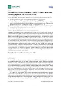
variables q f are computed, since their possible values must be below df0 . Without this specification, the solver would compute physical impossible results. The inverse functions of Table 2 are restricted to pure roll movements, as they contain a “balancing equation” for the two rear actuators. By restricting the front actuator (act3 ) the functions could also be used for pure roll movements instead. With the function QuasiStaticInverseStiffness is attempted to achieve stiffness control and the function uses the stiffness matrix that is derived in the previous section. One shortcoming of this method is that outer loads are excluded from the computation with this function. A quasi-static example computation involving the function QuasiStaticForward is given below. The callable functions that are used by the non-linear solver in other problems, are given in Appendix B.
Algorithm 2 Example computation of quasi-static solution (in) ~u, ~bi , ~si ∈ R3 , Rx (x), Ry (x) ∈ SO(3), J † ∈ R3×2 , c0 , df0 (out) x, q f 1: Init = 0 2: for l ≤ actuator range do 3: define q a from l and q a → QuasiStaticForward() 4: Sol = solve(QuasiStaticForward()) with Init as start value and qif ≤ df0 5: Init = Sol 6: function QuasiStaticForward(Input) 7: if intrinsic description then 8: R = Rx (Input1 ) · Ry (Input2 ) 9: if extrinsic description then 10: R = Ry (Input2 ) · Rx (Input1 ) 11: for i ≤ n do 12: Outputi = norm(~u + R · ~bi − ~si ) − (qia +Inputi+2 ) 13: τi = c0 ((df0 +Inputi+2 )−1.4 − (df0 −Inputi+2 )−1.4 ) 14: compute J † ← f (~u, ~bi , ~si , q a ,Input) 15: Output4 = (J †T · τ )1 16: Output5 = (J †T · τ )2 17: return Output
Variables written in capital letters indicate vectors or matrices that are created inside the computation with the exception of R.
23
3.7
Dynamic Model in OpenModelica
In addition to the derived models, the (free) software OpenModelica was used to create a comparative model. With help of the editor OMEdit and the libraries4 Multibody, Translational and Rotational a dynamic model was set up.
Figure 3.9: Depiction of model components in OMEdit representing one leg of the VSM. OMEdit comprises a block diagram depiction that is translated into Modelica syntax, which can also be accessed for a deeper specialisation of the model. This way, the modelling of pneumatic springs inside the language was achieved. Figure 3.9 shows the submodel of the overall mechanism, that can be defined in more detail in the “background” of the editor. In the present figure, the component force1 models the pneumatic spring in one leg of the VSM, whereas position1 serves for the forward actuator input that can be accessed from outside the model. One inconvenience of Modelica is that it aims at solving Ordinary Differential Equations (ODE) instead of Partial Differential Equations (PDE), where derivatives can only be described in terms of time. The inverse solution was not obtained, since it does not only incorporate the forces (like the forward model) but also 4
Modelica follows an object-oriented approach and its libraries therefore appear as classes in the system, bringing typical characteristics such as “inheritance” with them. For detailed information http: //book.xogeny.com/ can be consulted.
24
would need their position derivatives to solve the non-linear optimization problem. By defining the position input of the actuators, the forward solution can still be modelled and computed. With the Functional Mockup Unit (FMU), an export to the Python language is possible, which allows to carry out the simulation in this environment and specified input values. This model export is used as a comparison for the computations from the previously derived models.
Figure 3.10: Block diagram of the end-effector with applied damping in intrinsic configuration The dynamic modelling incorporates inertia forces and results in oscillations, that also occur in reality, but falsify the comparison with the quasi-static model. Since the masses and inertia cannot be set to zero in the OpenModelica model they are already defined with respect to the testbed design (see Section 5) to apply this model for further investigations. in order to prevent the model from oscillating during the simulation, a damping factor needs to be applied in roll and pitch joint of the end-effector. A depiction of the end-effector is given in Figure 3.10, here shown in intrinsic measurement configuration. To be seen are interface elements marked frame_a,frame_a1 and frame_a2 that 25
are used to connect this sub-model to the global one. Beside the introduced geometries and masses, the input values and the damping factors are also defined. Simulations under OpenModelica do not allow to retrieve data of end-effector stiffness and - comparable to realistic measurement - a predefined torque needs to be applied on the mechanism under which the deflection of the end-effector can be observed. Such an approach introduces a systematic error, further discussed in Section 4.7.
Section Summary: The derivation of analytical models led to workarounds that are necessary to apply. For example, the differential kinematics were obtained without the forward solution of the mechanism at hand, leading to a matrix that is dependent on the full set of generalized coordinates (Equation 3.7 and 3.9). A convenient model of the end-effector stiffness is derived by reducing the force expressions in Equation 3.18 with help of a pneumatic spring model to passive coordinates alone. Finally, a quasi-static end-effector model is shown which will serve as a comparison to the dynamic model build in OpenModelica.
26
4
Simulation and Results
This section covers the simulation of the mechanism with help of the models that were derived in Section 3. It will be shown that, first, the redundant actuation brings improvements on dexterity of the mechanism, and second that the idea of stiffness control is feasible. For the derivation of most kinematic expressions the sympy library of the programming language Python was used. Simulations were carried out with the derived functions and non-linear problems were solved with the scipy.optimize library. At first, an overview of the input data of the simulation is presented and subsequently the results of the non-redundant and redundant rigid designs are discussed. Eventually, the force and velocity transmissions of the rigid design are presented, followed by the study of the end-effector stiffness. The general simulations regarding the stiffness term are carried out with a maximum piston travel of df0 = 0.15 m to better show the stiffness behaviour under actuator changes. The gait cycle at the end of this section however, was simulated with an underlying travel of df0 = 0.015 m that was found as a suitable parameter under several simulations. Accordingly, this parameter is also chosen for the design described in Section 5. Finally, the simulation results from OpenModelica are put in contrast to the ones obtained in Python to verify the simulations.
4.1
Design Parameters
Before the computations with the derived models can be started, some input data must be available. They can be distinguished between geometry data which are roughly based on an existing design for the ankle mechanism in a humanoid robot at the DFKI, and biomechanical data about range, forces and velocities in human ankles. Geometric conception: In the first examination the geometry of the actuators is intentionally held simple to grasp a first understanding of the mechanism, rather to find an optimal design. Upper and lower attachment points of the actuators (vectors ~si and ~bi for i = 1, 2, 3) form equilateral triangles as to be seen in Figure 4.1. Both triangles are concentric and separated by a distance u, while the actuators are equally mounted by distances of 120 degree. The mounting of the third actuator is aligned with the x-axis and therefore with the rotation joint for roll movements.
27
Figure 4.1: Plot of the geometry in zero configuration inside numerical simulation. green: upper attachment structure, black: structure from {s}-frame to {b}-frame, red: lower attachment structure and blue: actuation legs Biomechanical data: Regarding dimensioning of the leg drives, the necessary speeds and torques in the ankle must be known. Also the necessary work range of the mechanism can be confined from biomechanical specifications. There exists a variety of scientific data that are partially selected and rounded for our purpose. Figure 4.2 shows the four main movements occurring in the human ankle to which most papers on human gait refer. Similar values were found by [17] and [32] with about 15◦ for dorsiflexion and about 5◦ of plantarflexion in normal walking. However, this value changes considerably for vertical jumps to a total range (dorsiflexion plus plantarflexion) of 79◦ as it was found by [41]. An interesting observation is that the ankle torque for walking with 1.8 Nm/kg and jumping with 1.6 Nm/kg is very similar [17] [12]. This means that under extension of the possible pitch work range, a design even suitable for jumping is formed. The work of [3] gives related data to the eversion and inversion of the foot, which have been averaged in torque and speed. A complete overview of collected values is given in Table 3 that serve for the design of the proposed mechanism. Inversion and eversion are comparatively small and could be - for the sake of better control possibilities and adaptability - doubled for the intended mechanism.
28
Table 3: Averaged ankle data from [17],[12], [32], [3] and [41]. Plantarflexion Dorsiflexion Eversion Inversion
range [deg] 20 60 5 5
speed [rad/s] 15 15 2.5 2.5
torque [Nm/kg] 1.8 1.8 0.25 0.25
Figure 4.2: Four main movements in the human ankle. Source: [11]
Further input parameters: For simplicity, the active actuator lengths are supposed to move in a range of 85-125 % of their lengths in zero pose. In turn, the pneumatic elements will be specified with a piston area of A = π/4 · 0.032 m2 and a value for df0 = 0.15 m that allows a full movement of all actuators simultaneously without exceeding the pneumatic pressure by five times the initial pressure of one atmosphere. Results to this simplified consideration are presented in Section 4.4 and are subject for the final discussion presented in Section 6.
4.2
Singularity and Dexterity for Rigid Design
A mechanism is singular when its Jacobian looses rank in a specific configuration - see e.g. [39](p.115). Thus the transformation between actuation and end-effector space is not defined any longer and the mechanism is either locked in its position or indeterminate. Such configurations must be avoided and can be identified by looking at the determinant or condition number of the Jacobian for a set of input values. The condition 29
number informs how close a configuration is to a singularity [5](p.321). Speaking about over-constrained systems, the work of [34] and [39] gives a criterion for manipulability with det(J J T ) = 0, where the manipulator Jacobian looses rank and a measure for the dexterity is described by the condition-index with 1/cond(J J T ).
Singularity - non-redundant
3
Condition index - non-redundant 1.0
2
roll [rad]
1 0.8
0 −1 −2
0.6
−3
3
Regions of very low dext. - redundant
Condition index - redundant 0.4
2
roll [rad]
1 0
0.2
−1 −2 −3 −3
−2
−1
0 pitch [rad]
1
2
3
−3
−2
−1
0 pitch [rad]
1
2
3
Figure 4.3: Comparison of manipulability and dexterity for the non-redundant and redundant design Figure 4.3 shows the improvements that are achieved by adding another actuator to the “original” non-redundant system. Singularities are fully eliminated from the workspace and the dexterity around the zero-configuration is improved. Since the mechanism will particularly used in this region, the redundant actuation itself has advantages over its 30
non-redundant counterpart. Regions of low dexterity 5 , as to be seen in the lower left of Figure 4.3 should however be avoided.
4.3
Velocity and Force Transmission for Rigid Design
To get an idea about the transmissivity of the ankle in terms of speed and torque, the biomechanical input data from Section 4.1 can be transformed into actuation space to prove the very general feasibility of the concept. Taking a constant input of these maximal values is approximate, but ensures to retrieve the upper bounds of actuator force and speed. Results of pitch and roll are separately computed and the mixed case is neglected for the sake of presentability, as to be seen in Figure 4.5 and 4.4. Those figures show the forces and velocities of the actuators for different configurations when the end-effector forces and velocities are given. Arising peaks in the force plots must not be confused with singularities, but with configurations of low dexterity, what also becomes clear from a look at the non-zero velocities in the same points. Force and speed expressions are independent of intrinsic or extrinsic description (see Section 3.2) and correspondingly are the simulation results.
τ1 τ2 τ3
0.10
work range
20
0.05
0
0.00
−20
da1̇ da2̇
−40
da3̇
−3
−2
−1
0 roll [rad]
1
2
actuator speed [m/s]
specific force [N/kg]
40
−0.05 −0.10
3
Figure 4.4: Actuator force and speed for pure roll movement when end-effector force and speed are given The power expression inside the actuation space can answer a more realistic design question for the actuators. Such plots can be found in Figure 4.7 and 4.6 - again separated for pitch and roll. While the roll movement of the foot demands an upper power limit 5
Low means when the condition index is in the interval [10−6 , 2 · 10−4 ].
31
200
1.5
work range
1.0
100
0.5
0
0.0
actuator speed [m/s]
specific force [N/kg]
2.0
τ1 τ2 τ3
300
−0.5
−100 −200
da1̇
−1.0
da3̇
−2.0
da2̇
−300 −3
−2
−1
0 pitch [rad]
1
2
−1.5
3
Figure 4.5: Actuator force and speed for pure pitch movement when end-effector force and speed are given of 0.32 W/kg for both rear actuators (act1 and act2 ), the defined pitch input results in a power limit of 18.5 W/kg for the front actuator (act3 ). This would result in an installed actuator power of almost 1200 W for the targeted robot RH5 from the DFKI with an approximate mass of 63 kg. Table 4: Design data of the actuators in rigid configuration with an underlying robot mass of 63 kg, separated for roll and pitch data. Maximum data are relevant direction roll pitch
force [N] 315 2623
velocity [m/s] 0.13 0.866
power [W] 19.86 1185
Such a demand is very high for an ankle construction and it raises the need for intrinsically different actuators to store and release energy - a need that could be fulfilled with VSMs. The topic of energy storage is however not covered by this work, but remains subject to further investigations of the VSM. An overview of specified motor parameters, arising from the transmission curves and the weight of the targeted robot is given in Table 4.
32
act1 act2 act3
work range
specific power [W/kg]
0.7 0.6 0.5 0.4 0.3 0.2 0.1 0.0
−3
−2
−1
0 roll [rad]
1
2
3
Figure 4.6: Power of all three actuators under pure roll movement when end-effector force and speed are given
act1 act2 act3
25
work range
specific power [W/kg]
20 15 10 5 0
−3
−2
−1
0 1 pitch [rad]
2
3
Figure 4.7: Power of all three actuators under pure pitch movement when end-effector force and speed are given
4.4
End-effector Stiffness
In Section 3.5 the derivation of the end-effector stiffness is detailed. It can be distinguished between active and passive terms that are partially shown in this section. Passive stiffness is generally the position dependent stiffness of the mechanism without any spring deflection involved. The mechanism is highly sensitive to the parameter df0 , which constitutes the stroke of the pneumatic springs and therefore introduces the non-linearity. 33
k [Nm/rad]
60 40 20
roll pitch
0
k [Nm/rad]
60 40 20 0
roll pitch −3
−2 −1 0 1 2 roll (upper fig.), pitch (lower fig.) [rad]
3
Figure 4.8: Stiffness changes for pure roll and pure pitch While it was found that a stroke of df0 = 0.015 m is suitable for the adaptation of a gait cycle by the ankle - simulated in Section 4.6 - this value is increased by factor ten in the quasi-static computation of Section 3.6. This is, because a bigger range of actuator movements is possible and the mixed influence of positional and forced stiffness is visible, as the actuator changes position and forces at the same time. Figure 4.8 depicts the stiffness behaviour under pure pitch and roll movement, also computed with a stroke of df0 = 0.015 m. In those two cases the values from the main diagonals of the stiffness matrix are identical to its eigenvalues in every point. A slight asymmetry in the bottom of Figure 4.8 can be observed, due to the installation of two actuators in the rear and one in the front when seen with respect to the pitch axis. A plot of the stiffness over the whole work range, separated for roll and pitch is given in Figure 4.9. It reveals that roll stiffness is well distributed over the work range, while the pitch stiffness shows best values in zero position and drops rather quickly in all directions. Such a behaviour is well suited for an ankle design, giving sufficient stability for roll and having a high pitch stiffness around the zero configuration. Because of the high non-linearity of the springs, this positional stiffness does not have a big impact on the overall stiffness that occurs under spring load (see stiffness values e.g. in Section 4.5).
34
Roll stiffness
3
Pitch stiffness 60
2
50
roll [rad]
1 40 0
30
−1
20
−2
10
−3 −2
−1
0 pitch [rad]
1
2
−2
−1
0 pitch [rad]
1
2
Figure 4.9: Roll and pitch stiffness (eigenvalues) over the complete work range. Colour variations are related to stiffness: k [Nm/rad]
4.5
Quasi-static computations
Some quasi-static computations with unique solution can be performed under a given actuator input. To benchmark the quality of the derived models, three different load cases are simulated with help of the function shown in Algorithm 2 and are compared in Section 4.7 with the dynamic model in OpenModelica. The quality of the solution also involves strongly the quality of the numerical solver. In the outlined examples the solver scipy.optimize.least_square was used. Similar results were obtained with scipy.optimize.fsolve, without setting bounds on the variables. It is because the structure of the forward problem is less demanding to the solver than for the inverse problem described in Section 4.6. Under a maximal spring stroke of df0 = 0.15 m and actuator changes in the range from ±30 % of their initial length, variantly one, two or three actuators are moved. These simulations aim at showing the coupled non-linearity of springs and kinematics of the system. Since also mixed load cases are involved in the third case, the eigenvalues of the stiffness matrix are shown in the resulting plots. Additionally, the actuator forces are given. For a long range of actuator movements, the end-effector angle changes and the force changes are almost linear under this comparable large spring stroke. In the load cases given by Figure 4.10 and 4.11 appears a clear transition point at around 0.375 m actuator displacement. It represents an interesting operating point, because the combined non-linearity of mechanism and spring keep roll and pitch angles at considerable constant values. Off diagonal values of the stiffness matrix were only found
35
k [Nm/rad]
in the mixed load case shown in Figure 4.11.
5.0 2.5
roll pitch
0.0
[rad]
1
roll pitch
0 −1
[N]
0
τ1 τ2 τ3
−50
0.225
0.250
0.275
0.300 d3a [m]
0.325
0.350
0.375
0.400
Figure 4.10: Stiffness, position and force changes by front actuator variation
k [Nm/rad]
15 10 5
roll pitch
0
[rad]
1 0
roll pitch
−1
[N]
100 0
τ1 τ2 τ3
−100 0.225
0.250
0.275
0.300
d2a,d3a [m]
0.325
0.350
0.375
0.400
Figure 4.11: Stiffness, position and force changes by front and one rear actuator variations
36
k [Nm/rad]
roll pitch
30 20 10 1e−9
[rad]
0.0 −0.5
200 [N]
roll pitch
0
τ1 τ2 τ3
−200 0.225
0.250
0.275
0.300
d1a, d2a, d3a [m]
0.325
0.350
0.375
0.400
Figure 4.12: Stiffness, position and force changes by three simultaneous actuator variations
4.6
Simulation of Human Gait
In order to bring the simulation closer to realistic cases, input data from a gait cycle can be fed to the system and the inverse solution can be computed to obtain the solution of the actuation variables q a and q f . In turn, the end-effector stiffness can be captured and displayed over the gait cycle. In Figure 4.13 a typical stance phase of one foot is given during walking. At zero stance, the foot touches the ground and leaves it at 100 % of the stance, whereas the maximum torque and deflection are reached at about 80 % stance. Recognisable in both curves is the positive peak before 20 % of the phase, often noted as heel strike, where the foot folds to the ground. Making use of Algorithm 4 a solution for the gait can be computed in every point of the stance phase. As already mentioned, it is important to restrict spring deflections q f to a maximal piston stroke of ± df0 during computation. Furthermore, the solution from previous calculation steps should be used as initial guess for the solver in the next step. For the inverse problem exists however an infinite set of solutions, each possessing different stiffness in roll and pitch. The solution presented in Figure 4.16 shows a clear stiffness increase at 75 % of the stance for both directions, as it can be observed in human ankles. With a curve crossing the value of 2000 Nm/rad, this stiffness increase lies approximately 1.5 times above usual values that were presented e.g. by [25]. 37
torque [Nm]
0 −25 −50 −75
torque data torque interpolation
−100
pitch [deg]
10
pitch data pitch interpolation
5 0 −5 −10 0
20
40
stance [%]
60
80
100
Figure 4.13: Resulting ankle torque and angle. Interpolation data according to [20]
0.32
d1a d2a d3a
0.30 0.28 0.01
d1f d2f d3f
0.00 −0.01
k [Nm/rad]
spr. defl. [m]
act. len. [m]
Alternatively, the pneumatic springs can be restricted during computation to obtain different results. In Figure 4.15 e.g. the solution of the gait cycle is shown, when the spring in the front leg (spr3 ) is restricted to 50 % of df0 . The loads are therefore adapted by the rear springs what results in a much higher stiffness characteristic for roll. To validate the obtained result, a back computation is carried out by using the solution as input for an altered quasi-static problem covered in Algorithm 3. Input torque and input angle are retrieved under the same stiffness curve and prove a correct computation. The plot is appended in Appendix D.
2000 roll pitch
1000 0
0
20
40 60 STANCE [%]
80
100
Figure 4.14: Non-unique solution for actuator and spring coordinates for gait cycle
38
act. len. [m]
d1a d2a d3a
0.30
d1f
0.00
d2f d3f
−0.01
k [Nm/rad]
spr. defl. [m]
0.32
roll pitch
5000 0
0
20
40
STANCE [%]
60
80
100
Figure 4.15: Non-unique solution for actuator and spring coordinates for gait cycle with front spring restricted to 50 % deflection
0.32
d1a d2a d3a
0.30
0.01110 d1f d2f
0.01105
−0.01125 −0.01130 −0.01135
k [Nm/rad]
spr. defl. [m]
spr. defl. [m]
act. len. [m]
A possibility to obtain unique solutions from the inverse quasi-static model is a direct control of the stiffness parameters by means of Algorithm 5. The same gait cycle was simulated with (arbitrarily) predefined roll stiffness of 900 Nm/rad and pitch stiffness of 800 Nm/rad and is given in Figure 4.16.
d3f
900 roll pitch
850 800
0
20
40
STANCE [%]
60
80
100
Figure 4.16: Unique solution for gait cycle under predefined stiffness
39
Three inconveniences come with this approach. First, a predefined stiffness is usually not the best criterion for a gait movement, instead, an energy optimization would be preferable. Second, this algorithm only leads to a solution when outer loads are neglected and movements are solely considered for one rotation axis. A mixed load case with K 6= diag(kββ , kγγ ) would thus be excluded. And third, as Figure 4.16 reveals, the spring deflections would need to be controlled physically on a very small interval, what is a difficult task under strong non-linearities.
4.7
Comparison with OpenModelica
Modelling in OpenModelica resulted in a forward dynamic model that was assessed to compare and check results from previous sections. The comparison with help of the load cases in Section 3.5 takes place to verify the theoretically derived stiffness term. Also the obtained inverse solution for the gait cycle, which was computed with Algorithm 2 is compared with the inverse solution of the rigid model in OpenModelica. For the simulations in OpenModelica, a damping factor of δ = 0.05 Nms/rad is applied on roll and pitch angle. The subsequent Figures 4.17 and 4.18 show the error in angle and force computation, related to the load cases that were performed in Section 3.6.
abs err. [rad]
0.000 −0.002 −0.004 roll pitch
−0.006
abs err. [rad]
0.10 0.05 0.00 −0.05
0.00 abs err. [rad]
roll pitch
1e−8
−0.25 −0.50 roll pitch
−0.75 0.24
0.26
0.28
0.30 changed actuator lengths [m]
0.32
0.34
0.36
Figure 4.17: Error in roll and pitch angle for three different load cases, as explained in the text. Upper plot: theoretical values, center plot: dynamic simulation from OpenModelica, bottom plot: relative error between both models
40
abs err. [N]
0.00 −0.05 −0.10
τ1 τ2 τ3
−0.15 −0.20
abs err. [N]
0
τ1 τ2 τ3
−1 −2 −3
abs err. [N]
0.015
τ1 τ2 τ3
0.010 0.005 0.000
0.24
0.26
0.28
0.30 changed actuator lengths [m]
0.32
0.34
0.36
Figure 4.18: Error in actuator forces for three different load cases, as explained in the text. Upper plot: theoretical values, center plot: dynamic simulation from OpenModelica, bottom plot: relative error between both models The first load case involves a constant movement of the front actuator by ± 20 % of its initial length, whereas the second case also has one rear actuator performing simultaneously the same movement. In the third load case, all three actuators are moved simultaneously. It is striking that the force errors are identical what suggests a systematic error between the models that is not of numerical origin. Even though, Considerable errors only occur in the mixed load case of simultaneous pitch and roll movement, becoming bigger when shifted towards stronger singularities. It can also be seen that the oscillations in the dynamic model persist during the first few simulation steps but decay due to introduced damping. To come close to the quasi-static case, a simulation time of 10 sec was used for the total actuator movements. To retrieve stiffness values from the OpenModelica model, an additional torque of 0.1 Nm is applied on roll and pitch joint. Then the end-effector deflections are compared to an unloaded simulation. This workaround creates systematic errors and is amplified by the application of damping in the system. For the simulations in OpenModelica, a damping factor of δ = 0.05 Nms/rad is applied on roll and pitch angle. Though, the results show comparable low error to the theoretical stiffness values. One exception is again when roll and pitch act at the same time - Figure 4.20. Whenever a simultaneous movement around roll and pitch joint occurs, the measurement torque must be applied individually for roll and pitch in two separate simulations to retrieve the 41
eigenvalues of the stiffness matrix. This is shown by the stiffness relation ∆f = K∆x ∆x = K −1 ∆f = Φ∆f with Φ as the compliance matrix. When load is only applied in one rotation direction at a time, the product of compliance matrix and force vector contains independent columns of Φ.
Φ · fβ xβ ββ = Φγβ · fβ xγ
for fγ = 0
Φ · fγ xβ βγ = Φγγ · fγ xγ
for fβ = 0
k [Nm/rad]
6
rel err. [%]
6
k [Nm/rad]
There are thus four independent equations that allow to compute all values of Φ from which the stiffness matrix can be retrieved by inversion. In Figure 4.19, 4.20 and 4.21 are the eigenvalues of the stiffness matrix shown for the previously mentioned load cases.
roll pitch
4
roll pitch
4
roll pitch
2.5 0.0 −2.5 0.24
0.26
0.28 0.30 0.32 changed actuator lengths [m]
0.34
0.36
Figure 4.19: Stiffness curves arising from changes in da1 . Upper plot: theoretical values, center plot: dynamic simulation from OpenModelica, bottom plot: relative error between both models
42
rel err. [%]
roll pitch
5.0
k [Nm/rad]
k [Nm/rad]
7.5
8 6
roll pitch
4
roll pitch
20 0 −20
0.24
0.26
0.28 0.30 0.32 changed actuator lengths [m]
0.34
0.36
rel err. [%]
k [Nm/rad]
k [Nm/rad]
Figure 4.20: Stiffness curves arising from changes in da1 and da2 . Upper plot: theoretical values, center plot: dynamic simulation from OpenModelica, bottom plot: relative error between both models
roll pitch
12.5 10.0 7.5
roll pitch
12.5 10.0 7.5
roll pitch
0.5 0.0 −0.5 0.24
0.26
0.28 0.30 0.32 changed actuator lengths [m]
0.34
0.36
Figure 4.21: Stiffness curves arising from changes in da1 , da2 and da2 . Upper plot: theoretical values, center plot: dynamic simulation from OpenModelica, bottom plot: relative error between both models For the load case depicted in Figure 4.20, a higher error can be seen, compared to the 43
symmetric load cases shown in Figure 4.19 and 4.21. The general validity of the stiffness term is given by the evaluated curves, since the error stays in acceptable bounds. During simulation with the model in OpenModelica, high errors in the forward simulation were detected that could not be corrected in the time span of this thesis. They are subject to future work on the simulations.
−0.6875
act1 act2 act3
−0.6900
relative error [%]
−0.6925 −0.6950 −0.6975 −0.7000 −0.7025 −0.7050 −0.7075 0
20
40
STANCE [%]
60
80
100
Figure 4.22: Error between rigid actuator lengths in OpenModelica and the quasi-static computations To achieve a comparison for the gait cycle computation of Section 4.6, a simplified rigid model was build in OpenModelica to verify the kinematic correctness of the gait-cycle results. Figure 4.22 shows the error between the rigid actuator length in OpenModelica and the total leg lengths (dai + dfi ) from the gait cycle computation. It can be concluded that the kinematic constraints are respected inside the quasi-static computation of Algorithm 2.
44
Section Summary: The previously derived models are assessed through different simulations, posing forward and inverse problems. Forward problems are present, when the variables of the actuation space q a are known. Inverse problems are closer to real life problems, when outer loads impose values on actuation space q a and deflection space q f . The latter case has no unique solution and must therefore be reformulated as a different optimization problem. Further investigations have to be pursued in this direction. The results are compared to a dynamic simulation in OpenModelica that needs to be adapted for a quasi-static solution. The adaptation comes with a cost of error introduction but shows sufficient good results. An in average higher error can be observed for mixed roll and pitch motions in all values. Difficulties in the computation of the gait-cycle were found in the simulation with OpenModelica and the model was thus reduced to a simpler rigid model to verify the kinematic constraints.
45
5
Design of a Test Environment
The presented mechanism in this thesis is a new design concept and there are no practical applications that have yet been tested. For the investigation of practical feasibility, a test setup will be used to implement stiffness control and also to gain first experiences with the new design. Operation and testing of that mechanism are not in the scope of this work, but a design for a test environment has been pursued.
Figure 5.1: Design of a variable test environment In Figure 5.1, an overview of this system is given in an isometric and diagonal side view. The structure is subdivided from the its middle by the end-effector of the system composed of a ring allowing pitch movements and a plate allowing roll movements. Above the end-effector, the actual VSM is implemented, consisting of three actuation legs, which are attached on the top plate and the end-effector. To impose movements and loads on the system, a non-redundant PM is used (control unit in Figure 5.1), that can be seen at the bottom of the arrangement. This is because mounting the drives and sensors of the end-effector in series to its joints would result in a far too heavy and complex design. For this reason, the drive and measurement mechanism itself is performed as PM. Upper and lower part of the system then only differ in the number of legs and in the equipment of the 46
pneumatic springs for the upper legs. The availability of standard universal joints and the motors, including gear boxes at the DFKI make this “mirrored” design an economic choice. Easy manufacturing and low priced standard parts are also considered for all remaining components. The kinematics of the control unit can be implemented by using the existing code and deleting one constraint equation (see Section 3.3).
5.1
Actuation Leg
One actuation leg consists of the gear box that drives a spindle and a fixed attachment of the pneumatic spring complemented by a sensor as shown in Figure 5.2. The kinematics of the real mechanism differ slightly to the specified kinematics of the simulation, as the spherical joint in the {b}-frame is replaced by an universal joint. This restriction is crucial, since the rotation of the spindle in the actuator possess an additional rotatory freedom. Not to block the spindle in a rotation around its axis would leave the actuator without effect. During conception, some importance was attached to the variability of geometric parameters of the system. Therefore, both attachment points of the actuation legs can be mounted in different positions in the fixed {s}-frame and the moving {b}frame - to be seen from the slots in the plates. In this aspect, the attachment points can also be formed to equilateral triangles, where every point is off any rotation axis. This case was not studied during simulation in Section 4, but could reveal deeper insight and even positive behaviour.
Figure 5.2: One actuation leg of the VSM with pneumatic element Force based control will be used to operate the mechanism, and therefore every actuation leg is equipped with one force sensor as to be seen in Figure 5.2. With help of the 47
analytic force law of the springs (Section 3.4) the spring deflection can be computed under negligence of friction. As additional information serve the absolute position sensors that are attached on the ring and plate of the end-effector. A detailed view is given in Figure 5.3 showing the sensor mountings as azure components, directly mounted on the rotation axis.
Figure 5.3: View of the end-effector of the system with mounted inductive sensors for the rotatory DOFs While the actuators deliver a force of 1200 N of force, the restricting components in the system are the pneumatic springs, being limited to a pressure of 10 bar. When calculating with a safety factor of 1.5, the motors must be roughly limited to an output force of 500 N. Based on this, structural load analysis and subsequent adaptation were carried out for the critical design parts and their results can be seen in Appendix C, revealing that the design can withstand the expected forces. The analysis was performed in the simulation environment of AUTOCAD - Inventor. Purchase parts are also listed in Appendix C, whereas technical drawings are not delivered with this work, since the foreseen production methods do not require them.
48
Section Summary: A cost-effective design for a testbed is proposed in this section, making use of already available components. To influence and measure the end-effector forces and positions, a rigid parallel mechanism is installed on the back side of the VSM. For future tests and applications, a force control is aimed and sufficient sensors are thus integrated in the design.
49
6
Conclusion and Outlook
In this work, a new kind of mechanism - labelled as Variable Stiffness Mechanism - has been proposed. Its purpose is to combine the advantages of PMs and VIAs, namely to have a compliant parallel structure with stiffness control ability. One goal, was to show that preferable stiffness behaviour can be achieved by introducing only one more actuator than end-effector DOFs. Under the perspective of redundant actuation and the accommodation of non-linear springs, a stiffness formulation for the end-effector of the mechanism - a humanoid ankle - was derived. For this purpose, the actuator forces in the ordinary stiffness equation were substituted by means of passive force equations coming from the springs. Arising from the need of active coordinated dependence, the spring coordinates are again expressed with the inverse kinematics. This substitution must only apply for the passive stiffness term, while it creates incorrect results in the active stiffness term. Meanwhile, the Jacobian of the mechanism is treated as for redundant actuation that keeps the spring coordinates as passive elements. This simplification is allowed since actuation DOFs and spring DOFs can be summed to one rigid body transformation. A positive feature of this mechanism is the removal of singularities in the workspace and accordingly, this mechanism can be fully described by numerical methods. It has been proved in the simulation results, that the derived stiffness expression is correct. Also, the usefulness of the quasi-static model has been shown. However, under asymmetric movements, a higher error in the quasi-static and stiffness model can be observed in comparison to a dynamic model from OpenModelica. During simulation, difficulties have been detected in the model that require further investigations. A restricted confrontation with the derived quasi-static and stiffness models was nevertheless possible and showed validity of those models. Simulations for human gait have been further performed, in which the mechanism showed a good adaptation to the outer loads. To have a useful advantage of the mechanism, an energy optimization was opted for the occurring inverse problem in a gait movement. Under the presented models,the solvability is only given with separate end-effector operations. A further criterion needs to be applied when e.g. roll movements are introduced in the gait. Based on the retrieved parameters from simulation, a testbed design was proposed. Design considerations lead to the incorporation of another PM in the testbed to apply loads and to measure forces for a force-based control. The obtained results show that the proposed idea of a VSM is feasible. Arising from the combined difficulties in theoretical treatment of PMs and involvement of non-linear elements, the models emerged to cumbersome expressions. E.g. the symbolic stiffness
50
equation includes 1416 trigonometric functions, while being a 2 × 2 matrix! This urgently demands for an alternative description of this mechanism. In [10] it is stated that spatial notation can cut the volume of algebra by a factor of 4 compared to standard 3D vector notation and should be one consideration for subsequent works. Moreover, [24] showed a successful application of screw theory on parallel-redundant structures. Advanced mathematical descriptions can help to achieve a computational simplification. In the following list, future steps are proposed that also comprise ideas that have not been examined within the scope of this work. • Improvements of the dynamical model in OpenModelica are necessary to have a fully consistent framework. • Changing the mathematical description to actual, advanced frameworks, such as Lie algebra to simplify the models. • Further investigating energy optimization as a general control criterion. • Simulations of off-axis arrangements - see Section 5. • Development of different non-linear springs that posses a non-asymptotic characteristic. This would reduce sensitive behaviour under strong non-linearities. • Dynamic simulations can be trailed more profoundly, as they showed interesting effects arising from the non-linear springs. This thesis may serve as a starting point for investigations in compliant parallel structures with all its possible applications in future robotics.
51
References [1] Alin Albu-Schäffer, Oliver Eiberger, Markus Grebenstein, Sami Haddadin, Christian Ott, Thomas Wimböck, Sebastian Wolf, and Gerd Hirzinger. Soft robotics adaptable compliance. IEEE Robotics & Automation Magazine, pages 20–30, 2008. [2] Joseph L. Awange and Erik W. Grafarend. Solving Algebraic Computational Problems in Geodesy and Geoinformatics. SPRINGER, Springer Heidelberg New York Dordrecht London, 2005. [3] Johanna E. Bischof, Alicia N. Abbey, Bavornrit Chuckpaiwong, James A. Nunley, and Robin M. Queen. Three-dimensional ankle kinematics and kinetics during running in women. Gait & Posture, 31:502–505, 2010. [4] Dimitar Chakarov. Study of the antagonistic stiffness of parallel manipulators with actuation redundancy. Mechanism and Machine Theory, 39:583–601, 2004. [5] Ward Cheney and David Kincaid. Numerical Mathematics and Computing. Thomson Brooks/Cole, Thomson Higher Education, 10 Davis Drive, Belmont, CA 940023098, 2008. [6] B. Vanderborght et al. Variable impedance actuators: A review. Robotics and Autonomous Systems, 61:1601–1614, 2013. [7] Grebenstein et al. The dlr hand arm system. IEEE International Conference on Robotics and Automation, pages 3175–3182, 2011. [8] Loeffl et al. The dlr c-runner: Concept, design and experiments. International Conference on Humanoid Robots, pages 758–765, 2016.
IEEE-RAS
[9] Sebastian Wolf et al. Variable stiffness actuators: Review on design and components. IEEE/ASME Transactions on Mechatronics, 21:2418–2430, 2016. [10] Roy Featherstone. Rigid Body Dynamics Algorithms. SPRINGER, 2008. [11] Amalea Fisher. Injury to innovation part i: Injury. https://www.tuneupfitness. com/blog/2017/04/05/injury-to-innovation-part-i-injury/. Accessed: 2017-12-12. [12] S. Fukashiroa and P.V. Komi. Joint moment and mechanical power flow of the lower limb during vertical jump. Int. J. Sports Med., 8:15–21, 1987. [13] Clement Gosselin and Jorge Angeles. Singularity analysis of closed-loop kinematic chains. IEEE Transaction on Robotics and Automation, 6:281–290, 1990. 52
[14] Sami Haddadin, Felix Huber, Kai Krieger, Roman Weitschat, Alin Albu-Schäffer, Sebastian Wolf, Werner Friedl, Markus Grebenstein, Florian Petit, Jens Reinecke, and Roberto Lampariello. Intrinsically elastic robots: the key to human like performance. IEEE/RSJ International Conference on Intelligent Robots and Systems, pages 4270–4271, 2012. [15] R. Van Ham, M. Van Damme, B. Verrelst, B. Vanderborght, and D. Lefeber. Maccepa, the mechanically adjustable compliance and controllable equilibrium position actuator: A 3dof joint with two independent compliances. International Applied Mechanics, 43:467–474, 2007. [16] Ronald Van Ham, Thomas G.Sugar, Bram Vanderborght, Kevin W.Hollander, and Dirk Lefeber. Compliant actuator designs. IEEE Robotics & Automation Magazine, -:81–94, 2009. [17] Andrew H. Hansen, Dudley S. Childress, Steve C. Miff, Steven A. Gard, and Kent P. Mesplay. The human ankle during walking: implications for design of biomimetic ankle prostheses. Journal of Biomechanics, 37:1467–1474, 2004. [18] Jianjun He, Hong Gu, and Zhelong Wang. Solving the forward kinematics problem of six-dof stewart platform using multi-task gaussian process. Journal of Mechanical Engineering Science, 227:161–169, 2012. [19] Neville Hogan. Impedance control: An approach to manipulation: Part iii - applications. Massachusetts Institute of Technology, Cambridge, March 1985. -. [20] M Hora, L Soumar, H Pontzer, and V Sladek. Body size and lower limb posture during walking in humans. Exp Brain Res, 114:71–85, 1997. [21] K.H. Hunt. Kinematic Geometry of Mechanisms. Oxford University Press, Walton Street, Oxford OX2 6DP, 1990. [22] Christine Vehar Jutte. Generalized synthesis Methodology of Nonlinear Springs for Prescribed Load-Displacement Functions. PhD thesis, University of Michigan, 2008. [23] Dan Kalman. A singularly valuable decomposition: The svd of a matrix. The American University Washington, DC 20016, February 2002. [24] Long Kang, Wheekuk Kim, and Byung-Ju Yi. Modeling and analysis of parallel mechanisms with both kinematic and actuation redundancies via screw theory. ASME Journal of Mechanisms and Robotics, 9:1–12, 2017.
53
[25] Robert F. Kirsch and Robert E. Kearney. Identification of time-varying stiffness dynamics of the human ankle joint during an imposed movement. PLoS ONE, 12:1– 26, 2017. [26] Sridhar Kota, Jinyong Joo, Zhe Li, Steven Rodgers, and Jeff Sniegowski. Design of compliant mechanisms: Applications to mems. Analog Integrated Circuits and Signal Processing, 29:7–15, 2001. [27] Shivesh Kumar, Abhilash Nayak, Heiner Peters, Christopher Schulz, Andreas Müller, and Frank Kirchner. Kinematic analysis of a novel parallel 2sprr+1u ankle mechanism in humanoid robot. In Marco Carricato, editor, Advances in Robot Kinematics, Cham, 2018. Springer Verlag GmbH. [28] Tae-Young Lee and Jae-Kyung Shim. Forward kinematics of the general 6-6 stewart platform using algebraic elimination. Mechanism and Machine Theory, 36:1073– 1085, 2001. [29] Mario Luces, James K. Mills, and Beno Benhabib. A review of redundant parallel kinematic mechanisms. Journal on Intelligent Robotic Systems, 198:86–175, 2017. [30] Kevin M. Lynch and Frank Park. Modern Robotics. Cambridge University Press, 2017. [31] M.T. Masouleh, D.R. Walter, M. Husty, and C. Gosselin. Solving the forward kinematic problem of 4-dof parallel mechanisms (3t1r) with identical limb structures and revolute actuators using the linear implicitization algorithm. ASME, pages 1– 10, 2011. DETC2011-47884. [32] Habib Masum, Subhasis Bhaumik, and Ranjit Ray. Conceptual design of a powered ankle-foot prosthesis for walking with inversion and eversion. Procedia Technology, 14:228–235, 2014. [33] J.-P. Merlet. Solving the forward kinematics of a gough-type parallel manipulator with interval analysis. The International Journal of Robotics Research, 23:221–235, 2004. [34] J.-P. Merlet. Jacobian, manipulability, condition number, and accuracy of parallel robots. ASME J Mech Des, pages 199–206, 2006. [35] J.-P. Merlet. Parallel Robots. SPRINGER, P.O. Box 17, 3300 AA Dordrecht, The Netherlands., 2006.
54
[36] Antonio Morell, Mahmoud Tarokh, and Leopoldo Acosta. Solving the forward kinematics problem in parallel robots using support vector regression. Engineering Applications of Artificial Intelligence, 26:1698–1706, 2013. [37] Andreas Mueller. Redundant actuation of parallel manipulators. Institute of Mechatronics at the Chemnitz University of Technology, March 1985. [38] Andreas Müller. Stiffness control of redundantly actuated parallel manipulators. IEEE International Conference on Robotics and Automation, 2006. [39] Richard M. Murray. A Mathematical Introduction to Robotic Manipulation. CRC Press, 1994. [40] Christian Ott, Alexander Dietrich, Daniel Leidner, Alexander Werner, Johannes Englsberger, Bernd Henze, Sebastian Wolf, Maxime Chalon, Werner Friedl, Alexander Beyer, Oliver Eiberger, and Alin Albu-Schäffer. From torque-controlled to intrinsically compliant humanoid robots. ASME Dynamic Systems & Control Magazine, 3:7–11, 2015. [41] Georgios Papaiakovou. Kinematic and kinetic differences in the execution of vertical jumps between people with good and poor ankle joint dorsiflexion. Journal of Sports Sciences, 31:1789–1796, 2013. [42] E.B. Paz, M. Ceccarelli, J.E. Otero, and J.L.M. Sanz. A Brief Illustrated History of Machines and Mechanisms. SPRINGER, 2010. [43] R. Penrose. A generalized inverse for matrices. Robotica, 8:105–109, 1990. [44] F. Pierrot, C. Reynaud, and A. Fournier. Delta: a simple and efficient parallel robot. Mathematical Proceedings of the Cambridge Philosophical Society, 51:406– 413, 1955. [45] S.Kock and W.Schumacher. A parallel x-y manipulator with actuation redundancy for high-speed and active-stiffness applications. International Conference on Robotics & Automation, pages 283–292, 1998. [46] S.Kock and W.Schumacher. A mixed elastic and rigid-body dynamic model of an actuation redundant parallel robot with high-reduction gears. International Conference on Robotics & Automation, pages 1918–1923, 2000. [47] Hamid D. Taghirad. Parallel Robots. CRC Press, 6000 Broken Sound Parkway NW, Suite 300, 2013. 55
[48] Giovanni Tonietti, Riccardo Schiavi, and Antonio Bicchi. Design and control of a variable stiffness actuator for safe and fast physical human/robot interaction. The American Mathematical MonthlyProc. IEEE ICRA Int. Conf. on Robotics and Automation, pages 526–531, 2005. [49] Godfried Toussaint. Simple proofs of a geometric property of four-bar linkages. The American Mathematical Monthly, 110:482–494, 2003. [50] Sebastian Wolf and Alin Albu-Schäffer. Towards a robust variable stiffness actuator. IEEE/RSJ International Conference on Intelligent Robots and Systems (IROS), pages 5410–5417, 2013. [51] Teresa Zielinska. Development of walking machines; historical perspective. Department of Power and Mechanical Engineering, Warsaw University of Technology, 00-665 Poland, 2004.
56
APPENDIX A - Results under Extrinsic Rotation This appendix presents plots of singularity, dexterity and stiffness when the rotatory movements are considered extrinsically. These parameters are thus description dependent. It also shows that there is a considerable difference and being clear about the rotations is thus of major importance.
Singularity - non-redundant
3
Condition index - non-redundant 1.0
2
roll [rad]
1 0.8
0 −1 −2
0.6
−3
3
Regions of very low dext. - redundant
Condition index - redundant 0.4
2
roll [rad]
1 0
0.2
−1 −2 −3 −3
−2
−1
0 pitch [rad]
1
2
3
−3
−2
−1
0 pitch [rad]
1
2
3
Singularity curves and dexterity of the mechanism in non-redundant and redundant design
57
k [Nm/rad]
6 4 2
roll pitch
0 k [Nm/rad]
6 4 2 0
roll pitch −3
−2 −1 0 1 2 roll (upper fig.), pitch (lower fig.) [rad]
3
Positional stiffness of the mechanism, separately for roll and pitch
Roll stiffness
3
Pitch stiffness 8
2
7 6
roll [rad]
1
5 0
4 3
−1
2 −2
1
−3 −2
−1
0 pitch [rad]
1
2
−2
−1
0 pitch [rad]
1
2
Positional stiffness of the mechanism over whole workrange
58
APPENDIX B - Simulation Algorithms
Algorithm 3 Callable function structure for the full forward quasi-static model (in) q a , q f ∈ Rn (out) x, f 1: function QuasiStaticForwardFull(Input) 2: if intrinsic description then 3: R = Rx (Input1 ) · Ry (Input2 ) 4: if extrinsic description then 5: R = Ry (Input2 ) · Rx (Input1 ) 6: for i ≤ n − 1 do 7: Outputi = norm(~u + R · ~bi − ~si ) − (qia + qif ) 8: for i ≤ n do 9: τi = c0 ((df0 + qif )−1.4 − (df0 − qif )−1.4 ) 10: compute J † ← f (~u, ~bi , ~si , q a ,Input1,2 ) 11: Output3 = (J †T · τ )1 −Input3 12: Output4 = (J †T · τ )2 −Input4 13: return Output
Algorithm 4 Callable function structure for the inverse quasi-static model (in) x, f ∈ Rm (out) q a , q f 1: function QuasiStaticInverse(Input) 2: if intrinsic description then 3: R = Rx (x1 ) · Ry (x2 ) 4: if extrinsic description then 5: R = Ry (x2 ) · Rx (x1 ) 6: for i ≤ n do 7: Outputi = norm(~u + R · ~bi − ~si ) − (Inputi Inputi+3 ) 8: τi = c0 ((df0 +Inputi+3 )−1.4 − (df0 −Inputi+3 )−1.4 ) 9: compute J † ← f (~u, ~bi , ~si , x,Input) . for i = 1, ..., n 10: Output4 = (J †T · τ )1 − f1 11: Output5 = (J †T · τ )2 − f2 12: Output6 = Input1 =Input2 . No roll movement is allowed 13: return Output
59
Algorithm 5 Callable function structure for the inverse quasi-static forward model under stiffness predefinition (in) x, f ∈ Rm kββ , kγγ ∈ R (out) x, f 1: function QuasiStaticInverseStiffness(Input) 2: if intrinsic description then 3: R = Rx (x1 ) · Ry (x2 ) 4: if extrinsic description then 5: R = Ry (x2 ) · Rx (x1 ) 6: for i ≤ n do 7: Outputi = norm(~u + R · ~bi − ~si ) − (Inputi Inputi+3 ) 8: compute K ← f (~u, ~bi , ~si , x,Input,df0 , c0) . for i = 1, ..., n 9: Output4 = K0,0 − kββ 10: Output5 = K0,0 − kγγ 11: Output6 = Input1 =Input2 . No roll movement is allowed 12: return Output
60
APPENDIX C - Testbed Design Data The shown Finite Element Simulations are based on a maximal actuator force of 500 N when the actuators are expected to transmit the load in the most unpropitious configuration on the metal plates. All results in stress and displacement are in an acceptable range. Stainless steel is chosen as material for the depicted parts. Below, the exact ID and producer of the pneumatic elements and the sensors are given: Landefeld Druckluft und Hydraulik GmbH Konrad-Zuse-Straße 1 34123 Kassel-Industriepark Deutschland
ID: SQ 32/15 SZ
Burster Präzisionsmesstechnik GmbH & CO KG Talstraße 1-5 76593 Gernsbach Deutschland
ID: 8431-5010
61
62
0 −50
roll pitch
−100
k [Nm/rad]
angle [deg]
torque [Nm]
APPENDIX D - Back Computation of Gait Cycle
10
roll pitch
0 −10 roll pitch
2000 1000 0
0
20
40
stance [%]
60
80
100
Results from the back computation of the gait cycle, performed with the solution values of the inverse problem as input
63