Recent Techniques in Educational Science
Confidence intervals for Cronbach’s reliability coefficient 1
MICHAIL TSAGRIS1, CONSTANTINOS C. FRANGOS2, CHRISTOS C. FRANGOS3 School of Mathematical Sciences, University of Nottingham, Nottingham, UNITED KINGDOM
[email protected] 2 Division of Medicine, University College London, London, UNITED KINGDOM
[email protected] 3 Department of Business Administration Technological Educational Institute of Athens, Athens, GREECE
[email protected]
Abstract: - Cronbach’s alpha reliability coefficient was suggested as measure of the internal consistency of a questionnaire. The focus of this work is on the interval estimation of the alpha coefficient. Iacobucci and Duhachek (2003) and Koning and Franses (2006) explored transformations for constructing confidence intervals for the true value of alpha based on the asymptotic distribution of the estimate of the coefficient van Zyl et al. (2000). Padilla et al. (2012) examined confidence intervals for the alpha coefficient using bootstrap with non normal populations. We provide an alternative transformation of the alpha coefficient and construct confidence intervals for the true value. In order to do this we also employ the asymptotic distribution of the estimate of the coefficient van Zyl et al. (2000). Simulation studies are performed to demonstrate our methodology when the data are continuous and when they are converted to a Likert scale. A comparison with some present methodologies including the bootstrap methodology is presented as well. Key-Words: - reliability, Cronbach’s alpha, transformation, asymptotic normal, delta method, confidence intervals divided by the observed (through a measurement) value. Lord and Novick [2] starting from this suggestion they created the classical psychometric theory of the true value. According to them, the measurement X has two components, the true value T and the measurement error : X T . The reliability is used as a tool of estimating the percentage of the true value in a measurement, that is
1 Introduction The term repeatability refers to the replication of an experiment or test under different circumstances and the reproducibility refers to the conduction of the experiment or test by another person. In both cases, the measurements should have small deviations from replication to replication. If the latter is true, then there are grounds to believe that the measurement is very accurate and the measurement errors are rather small. This means that the procedure can be thought of as being reliable. If a test for instance is administered to some people more than once and the results do not differ significantly, then the test can be assumed to have high reliability or being reliable. The term reliability though is due to Spearman [1], who first said that errors exist even in the non sampling cases. He noted that these errors can be estimated by the size of consecutive and repetitive measures. Each measurement consists of two elements, the true value of the measurement and the error of the measurement. If the measurement is repeated it will yield new values both for the measurement and the error associated with it. The reliability is actually the ratio of the true value
ISBN: 978-1-61804-187-6
Re liability
True value T Observed Value X
(1)
Since the replication of a test is not always feasible, another term has been added in the literature, the internal consistency. This means that one must treat the same test as it had been administered twice and estimate the reliability of it. Due to this replication difficulty many reliability coefficients have been suggested over the years. In this work, Cronbach’s reliability coefficient, also known as Cronbach’s alpha or alpha coefficient is under consideration. We will examine some of the proposed ways of constructing confidence intervals for the true value of the alpha coefficient and suggest a new way. All ways will be compared via simulation studies in
152
Recent Techniques in Educational Science
estimate. The asymptotic 1 / 2% confidence interval in this case has the classical formula
terms of the level of coverage with the focus being on the low sample size cases. We will see the performance of the methods when the data are continuous and when they are converted to a Likert scale.
ˆ
1 / 2
Varˆ ( ˆ ) , ˆ 1 / 2 Varˆ ( ˆ )
(4)
where 1 / 2 is the 1 / 2 quantile of the
2 Cronbach’s reliability coefficient
standard normal distribution. We will refer to (4) as the ID confidence interval.
Cronbach’s reliability coefficient was suggested as measure of the internal consistency of a questionnaire [3]. The test cannot always be applied twice (in order to see variance between the two measurements X . For this reason Cronbach’s alpha is to be used. The formula of the Cronbach’s alpha reliability coefficient is the following
3.2 Confidence interval suggested by Koning and Franses van Zyl et al. [4] mentioned that under the assumption of compound symmetry and by using the delta method
p p p Y j 1 Var ( Y ) Var (2) j p 1 j 1 j 1 where Y j stands for the j-th variable Y (or j-th
1 p (5) 1 d n log1 ˆ log1 N 0 , 2 2 2 p 1
item/question). Koning and Franses [5] used (5) to derive a stable confidence interval
3 Confidence intervals for the alpha coefficient
2
j Sj T
3
j Sj trS T
2
Bias corrected and accelerated confidence intervals (BCa) were suggested by Efron [6, 7]. They are an improved form of non-parametric confidence intervals. The percentile method relies on calculating the lower and upper ( / 2 )% of the bootstrapped sample estimates of the parameter of interest [6, 7, 8].
(3),
tr S 2trS j S j 2
T
2
ˆ
ISBN: 978-1-61804-187-6
/2
, ˆ 1 / 2
(7)
where the upper script indicates the bootstrap sample estimate. The BC a is a improved version of (7)
The S stands for the sample unbiased estimator of the true covariance matrix (Σ) of the items, tr indicates the trace of a matrix j is a p dimensional vector of ones and n is the sample size. If the items are parallel (the covariance matrix has compound symmetry), then simplifies to 2 2 p 11 ˆ p , where ˆ
(6)
3.3 Non parametric bootstrap confidence interval
Van Zyl at al. [4] derived the variance of the distribution of the sample alpha coefficient assuming normality of the estimator. The formula for the estimated variance is
p2 2 n p 1
We will refer to (6) as the KF confidence interval.
3.1 Confidence interval based on the asymptotic normal distribution of the sample alpha coefficient
Varˆ ( ˆ )
1 1 ˆ exp 1 / 2 2 p n p 1 , 1 1 ˆ exp 1 / 2 2 p n p 1
The alpha coefficient provides a point estimate of the reliability. Being an estimate of the true reliability, its standard error should be given as well leading to an interval estimation of the true value. The alpha is only an estimate of the true value.
ˆ
1
, ˆ 2
(8)
1 aˆ ˆz 1 aˆ ˆz Z
where 1 ˆz 0 ˆz 0 Z / 2
2 ˆz0 ˆz0 Z1 / 2
is the sample
153
0
0
Z / 2 ,
1 / 2
,
Recent Techniques in Educational Science
for obtaining confidence intervals for Cronbach’s alpha. The important feature of the simulations is to see the performance of the methods in the low sample case. We start with a given covariance matrix and a known value of Cronbach’s alpha and generate 10,000 samples from a multivariate normal distribution with the covariance matrix. Each time we estimate the Cronbach’s alpha using (2) and then construct confidence intervals using the four aforementioned methods. We estimate the true coverage of each confidence interval from the proportion of times a confidence intervals includes the true value of alpha. The nominal coverage is set to 1 / 2 0.95 and hence, when the estimate
is the standard normal cumulative distribution ˆ are the bias correction and function and ˆz 0 and a acceleration terms respectively. The value of the bias correction term is calculated from the proportion of bootstrap estimates less than the [6], original estimate ˆ 1 ˆz 0 # ˆ b ˆ B , where ˆ b indicates
the b th bootstrap sample estimate of the alpha and B is the number of bootstrap samples. The acceleration term is calculated from the original sample using the jackknife. Let ˆ i denote the sample
estimate
of
alpha
when
observation is deleted and ˆ
i th
the
n
ˆ
n . Then, a
lies within 0.946 , 0.954 we will say the method achieves the nominal coverage. The procedure will be repeated for sample sizes ranging from 15 up 1000 for two covariance matrices and the number of dimensions for each case is equal to 5. In reality however, the questionnaires consist of ordinal data and not continuous. Hence, for each sample we will transform the continuous data into categorical and repeat the same estimating procedure. For simulated data set, we categorized each of the variables using the 15%, 30%, 60% and 75% quantile points. The first 15% of the data were assigned to the first category, the next 15% of the data to category 2 and so on.
1
simple expression for the acceleration constant is
aˆ ˆ ˆ n
3
i 1
n 2 6 ˆ ˆ i 1
3/ 2
.
3.4 Logit confidence interval We suggest a new confidence interval based on the logit transformation. The logit transformation is generally used for numbers within (0,1); proportions for example. The reliability estimates the percentage of the true value in a measurement (1) and thus is a proportion. Cronbach’s reliability coefficient (2) is a number within (0,1). Hence, ˆ logˆ 1 ˆ and via the delta method
2 Varˆ ˆ 1 ˆ 1 1 ˆ Varˆ ˆ , where Varˆ ˆ is defined in (3). An asymptotic
1 / 2%
ˆ
low
4.1 Example 1: Clamwest data We used the data taken from Aitchison [9]. It is a 20 x 6 data set consisting of Colour-size compositions of 20 clam colonies from West Bay. Since the data are compositional (i.e. each row vector sums to 1) we transformed them using the alpha-transformation with alpha=-1. The correlation matrix can be supplied by the authors. The resulting Cronbach’s alpha was equal to 0.641. Table 1 summarizes the estimated coverages of the 4 methods when the data are continuous. We can see the logit method (10) performs very well it attains the coverage level even for sample sizes. BCa had on average the lowest coverage. Casella and Berger (2001) do not suggest the use of bootstrap methodology for estimating the variance of the variance. We cannot say with certainty that this is the case for the alpha coefficient even though it is a function of variances. Table 2 presents the estimated coverages after the data have been transformed to the ordinal scale. The results do not look so good and in fact when the sample size is 1000 the estimated coverages are very
confidence interval for is given by
ˆ ˆ ˆ 1 / 2 Va r( ) , ,ˆ up ˆ ) ˆ ˆ Va r ( 1 / 2
(9)
Finally, an asymptotic 1 / 2% confidence interval for (denoted by LCI) is given by backtransforming the end points of (9)
exp ˆlow exp ˆup , ˆ ˆ 1 exp low 1 exp up
(10)
4 Simulation studies We perform simulation studies in order to examine the coverage accuracy of each of the four methods
ISBN: 978-1-61804-187-6
154
Recent Techniques in Educational Science
Table 1. Estimated coverages of the 4 methods when the data are continuous. Bold numbers indicate the estimated coverage was within the acceptable limits. Methods ID KF BCa Logit Estimated alpha
Sample sizes 15 25 0.922 0.933 0.978 0.987 0.888 0.918 0.951 0.956
40 0.943 0.99 0.93 0.954
50 0.947 0.991 0.941 0.957
100 0.947 0.993 0.94 0.95
500 0.947 0.992 0.945 0.949
1000 0.953 0.995 0.953 0.954
0.606
0.628
0.633
0.637
0.641
0.641
0.623
Table 3. Estimated coverages of the 4 methods when the data are continuous. Bold numbers indicate the estimated coverage was within the acceptable limits. Methods ID KF BCa Logit Estimated alpha
Table 2. Estimated coverages of the 4 methods when the data are ordinal with 5 categories. Bold numbers indicate the estimated coverage was within the acceptable limits. Methods ID KF BCa Logit Estimated alpha
Sample sizes 15 25 0.896 0.908 0.922 0.937 0.901 0.924 0.952 0.947
40 0.923 0.948 0.941 0.954
50 0.918 0.947 0.94 0.946
100 0.916 0.945 0.935 0.934
500 0.863 0.895 0.883 0.874
1000 0.813 0.844 0.83 0.824
0.613
0.642
0.648
0.652
0.658
0.658
0.635
40 0.941 0.94 0.929 0.947
50 0.951 0.95 0.938 0.953
100 0.947 0.944 0.938 0.946
500 0.944 0.943 0.944 0.944
1000 0.948 0.948 0.947 0.948
0.809
0.827
0.83
0.833
0.835
0.836
0.822
Table 4. Estimated coverages of the 4 methods when the data are ordinal with 5 categories. Bold numbers indicate the estimated coverage was within the acceptable limits. Methods ID KF BCa Logit Estimated alpha
low. If we take a look at the last rows of each table we will see that the estimated alpha (averaged over the 10,000 simulations for each sample size) reaches the true value of alpha as the sample size increases. This is the case for the continuous data but not for the ordinal data. For the ordinal data, when the sample sizes increases, on average the estimated alpha overestimates the true value of alpha.
Sample sizes 15 25 0.944 0.954 0.927 0.938 0.919 0.933 0.962 0.953
40 0.961 0.937 0.938 0.948
50 0.964 0.943 0.942 0.953
100 0.958 0.927 0.928 0.935
500 0.881 0.851 0.845 0.858
1000 0.792 0.76 0.75 0.765
0.803
0.818
0.82
0.822
0.825
0.825
0.814
coverage was within the acceptable limits. However this conclusion is based on two small scale simulation studies and further simulation studies need to be performed in order to have a clearer picture. In these simulations three of the suggested (in the literature) confidence intervals did not perform very well when the sample sizes are small. When the data are transformed to a Likert-type scale the results seem to have no validity. The estimated coverages of all methods are low. In this case the question of consistency and the unbiasedness properties of the estimator of alpha are raised. The present simulation studies showed that there is bias in the estimation of alpha when the data are in a Likert scale. This explains possibly partially why the coverage of the methods was so low. The problem of bias of the estimator of alpha is not new. Zumbo et al. [11] suggested that the alpha estimator (2) should be applied to the polychoric correlation matrix of the data. We have not included other ways of obtaining confidence intervals, such as the Asymptotically Distribution-Free (ADF) method of MaydeuOlivares et al. [12]. We are working towards including more methods in a larger scale simulation study. The final goal is to construct a hypothesis testing for the true lower bound of alpha.
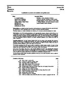
4.2 Example 2: Open-closed book data The second example uses the open-closed book data [10]. The correlation matrix of this data can be provided by the authors. The alpha coefficient is equal to 0.836 based on this dataset. The results for the estimated coverages when the data are continuous are similar to the ones obtained before. The logit method (10) performs very well, even when the sample size is low. Its estimated coverage is almost constant around 0.95, whereas the other methods need a larger sample size to attain the nominal coverage level. When the data are transformed into the ordinal scale, results are not as good in this case either. The estimated coverage of the 4 methods is lower than the nominal one for large sample sizes. If we see the estimated alpha coefficients for all the sample sizes we will see that when the data are continuous, the estimate equals the true value of alpha. On the other hand, when the data are ordinal, there is an underestimation of the true value of alpha.
References: [1] Spearman, C., General intelligence, objectively determined and measured, American Journal of Psychology, Vol.15, No.2, 1904, pp. 201-292. [2] Lord, F., Novick, M., Statistical theories of mental test scores. Addison-Wesley, 1968.
5 Conclusions At first we can say that the logit transformation produced confidence intervals whose estimated
ISBN: 978-1-61804-187-6
Sample sizes 15 25 0.928 0.935 0.929 0.94 0.905 0.921 0.958 0.949
155
Recent Techniques in Educational Science
[3] Cronbach, L., Coefficient alpha and the internal structure of tests, Psychometrika, Vol.16, No.3, 1951, pp. 297-334. [4] van Zyl, J., Neudecker, H., Nel, D., On the distribution of the maximum likelihood estimator of Cronbach’s alpha, Psychometrika, Vol.65, No.3, 2000, pp. 271-280. [5] Koning, A., Franses, H. P., Confidence intervals for Cronbach's coefficient alpha values. Technical report, Erasmus Research Institute of Management – ERIM, 2006. [6] Efron, B., Tibshirani, R.J., An introduction to the bootstrap, Chapman & Hall CRC, 1993. [7] Frangos, C. C., An updated bibliography on the jackknife method, Communications in Statistics-Theory and Methods, Vol.16, No.6, 1987, pp. 1543-1584. [8] Tsagris, M., Elmatzoglou, I., Frangos, C. C., The Assessment of Performance of Correlation
Estimates in Discrete Bivariate Distributions Using Bootstrap Methodology, Communications in Statistics - Theory and Methods, Vol.41, No.1, 2012, pp. 138-152. [9] Aitchison, J., The Statistical Analysis of Compositional Data, Springer Netherlands, 1986. [10] Mardia, K. V., J. T. Kent, J. M. Bibby. Multivariate analysis, Academic Press, 1979. [11] Zumbo, B. D., Gadermann, A. M., Zeisser, C., Ordinal versions of coefficients alpha and theta for Likert rating scales, Journal of Modern Applied Statistical Methods, Vol.6, No.1, 2007, pp. 21-29. [12] Maydeu-Olivares, A., Coffman, D., Hartmann, W.,. Asymptotically distribution-free (ADF) interval estimation of coefficient alpha, Psychological Methods, Vol.12, No.2, 2007, pp. 157-176.
Appendix
Fig 1. Estimated coverages for Example 2 when data are (a) continuous and (b) ordinal.
Fig 2. Estimated coverages for Example 2 when data are (a) continuous and (b) ordinal.
ISBN: 978-1-61804-187-6
156