Confidence intervals for the duration of a mass extinction

Paleobiology, 38(2), 2012, pp. 265–277

Confidence intervals for the duration of a mass extinction Steve C. Wang, Aaron E. Zimmerman, Brendan S. McVeigh, Philip J. Everson, and Heidi Wong

Abstract.—A key question in studies of mass extinctions is whether the extinction was a sudden or gradual event. This question may be addressed by examining the locations of fossil occurrences in a stratigraphic section. However, the fossil record can be consistent with both sudden and gradual extinctions. Rather than being limited to rejecting or not rejecting a particular scenario, ideally we should estimate the range of extinction scenarios that is consistent with the fossil record. In other words, rather than testing the simplified distinction of ‘‘sudden versus gradual,’’ we should be asking, ‘‘How gradual?’’ In this paper we answer the question ‘‘How gradual could the extinction have been?’’ by developing a confidence interval for the duration of a mass extinction. We define the duration of the extinction as the time or stratigraphic thickness between the first and last taxon to go extinct, which we denote by D. For example, we would like to be able to say with 90% confidence that the extinction took place over a duration of 0.3 to 1.1 million years, or 24 to 57 meters of stratigraphic thickness. Our method does not deny the possibility of a truly simultaneous extinction; rather, in this framework, a simultaneous extinction is one whose value of D is equal to zero years or meters. We present an algorithm to derive such estimates and show that it produces valid confidence intervals. We illustrate its use with data from Late Permian ostracodes from Meishan, China, and Late Cretaceous ammonites from Seymour Island, Antarctica. Steve C. Wang, Aaron E. Zimmerman,* Brendan S. McVeigh,** Philip J. Everson, and Heidi Wong.*** Department of Mathematics and Statistics, Swarthmore College, Swarthmore, Pennsylvania 19081, U.S.A. E-mail: [email protected]. *Present address: Department of Statistics, University of Washington, Box 354322, Seattle, Washington 98195. **Present address: The Brattle Group, 1850 M Street NW, Washington, D.C. 20036. ***Present address: Fairfax & Sammons Architects, 67 Gansevoort Street, New York, New York 10014 Accepted: 3 August 2011

Introduction Ever since the landmark paper of Alvarez et al. (1980), there has been much interest in determining whether the fossil record at a locality is consistent with a sudden and catastrophic extinction. This task, however, is complicated by the incompleteness of the fossil record. Even if a set of taxa went extinct simultaneously, their last appearances in a stratigraphic section may nonetheless appear gradual (Signor and Lipps 1982). Using statistical methods, several authors have accounted for this Signor-Lipps effect in testing whether a pattern of fossil occurrences is consistent with a simultaneous extinction (Meldahl 1990; Marshall 1995a; Marshall and Ward 1996; Solow 1996; Rampino and Adler 1998; Jin et al. 2000; Solow and Smith 2000; Groves et al. 2005; Ward et al. 2005). In such tests, several issues arise: 1. In classical statistical hypothesis testing, the two competing hypotheses are not treated equally. Rather, the null hypothesis ’ 2012 The Paleontological Society. All rights reserved.

is privileged in the sense that it is the default, and it is not rejected unless one can disprove it beyond a reasonable doubt (which typically means having a p-value less than the standard alpha level of 0.05). In some situations, this asymmetry of the null and alternative hypotheses is desirable—for instance, in a clinical trial we may not want to recommend a new drug treatment unless it can be conclusively shown to work better than an existing treatment. In other situations, however, we may not want to favor either hypothesis a priori. 2. Even if one accepts the classical hypothesis testing setup, it is not clear which scenario—sudden or gradual extinction— should be taken as the null hypothesis in testing for a mass extinction. In most papers, sudden extinction is the null and assumed correct until proven otherwise (although see Solow and Smith 2000). But this choice causes the test to favor simultaneous extinction unless strong evidence for gradual extinction exists. It 0094-8373/12/3802–0005/$1.00

266

STEVE C. WANG ET AL.

may actually be more reasonable to make sudden extinction the alternative hypothesis, because that is usually the research hypothesis—the hypothesis investigators set out to demonstrate. But this is technically difficult, because ‘‘gradual extinction’’ is not a single scenario, but a range of possibilities. ‘‘Sudden extinction,’’ on the other hand, is a point hypothesis and therefore more tractable as the null hypothesis, so it becomes a convenient default even though it may not always be appropriate. 3. Sudden and gradual are a false dichotomy. No mass extinction event is truly simultaneous; there is always some duration, however short, separating the first and last extinctions. Furthermore, the distinction between sudden and gradual is arbitrary and depends on context. For example, a paleontologist might consider the endCretaceous extinction sudden even if it lasted 10,000 years, whereas a biologist might consider the extinction of an island species gradual if it occurred over 500 years following human colonization. 4. Even if the fossil record is consistent with a sudden extinction, it may also be consistent with a range of gradual extinctions as well. That is, even if the null hypothesis is not rejected, it is a fallacy to infer that the null hypothesis is therefore true, and that the extinction must have been simultaneous. Consider an analogy with the American criminal justice system. Because defendants are considered innocent until proven guilty, the null hypothesis is that the defendant is innocent. If the prosecution cannot establish guilt beyond a reasonable doubt, then we fail to convict the defendant, who is found not guilty. But ‘‘not guilty’’ is not synonymous with ‘‘innocent.’’ A jury may well believe that the defendant is in fact guilty but simply lack sufficient evidence to convict, which is a different matter from believing that the defendant is innocent. 4. Similarly, we may conclude that the fossil record is consistent with a simultaneous extinction because we lack sufficient evidence to refute such a null hypothesis. But that does not mean that the extinction

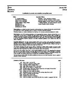
is not also consistent with a gradual extinction. In fact, any set of fossil occurrences that is consistent with a simultaneous extinction is also consistent with some range of gradual extinctions. For example, Jin et al. (2000) concluded that the fossil occurrences of Late Permian ostracodes of Meishan, China, were consistent with a sudden (simultaneous) extinction (Fig. 1A). However, they are also consistent with a gradual extinction (Fig. 1B)—more consistent, in fact, because the gap on the end of each taxon’s stratigraphic range is smaller. We attempt to resolve these issues by reframing the hypothesis test using a confidence interval framework. Rather than being limited to rejecting or not rejecting a particular scenario, we estimate the range of extinction scenarios that is consistent with the fossil record. In other words, rather than testing the simplified distinction of ‘‘simultaneous versus gradual,’’ we ask, ‘‘How gradual?’’ We answer this question by deriving a confidence interval for the duration of a mass extinction—the difference (in time or stratigraphic distance) between the first and last taxon to go extinct in a stratigraphic section. We are thus able to say, within a statistically rigorous framework, that the fossil record in a locality is consistent with a range of extinctions occurring over, for example, 0.3 to 1.1 million years of time, or over 24 to 57 meters of stratigraphic thickness. We emphasize that this viewpoint does not deny the existence of a genuinely simultaneous extinction; rather, in our framework, a simultaneous extinction is one whose duration is zero years or meters. Our goal is to estimate how long the extinction event lasted, rather than when it occurred. The need for such an estimate has been recognized previously, but currently there is no standard methodology for computing confidence intervals for the duration of an extinction event. Wang (2001) proposed the idea on which the current paper is based, but did not actually implement a working method. Payne (2003: p. 43) wrote: [O]ne would ideally… define the range of extinction scenarios compatible with the fossil record, rather than being limited to

DURATION Of A MASS EXTINCTION

267

FIGURE 1. Fossil occurrences of ostracodes from the Late Permian of Meishan, China (Jin et al. 2000). Units are millions of years after the beginning of the section. A, The observed fossil occurrences are consistent with a simultaneous extinction of all taxa at the given position (horizontal line) using a likelihood ratio test (Solow 1996; Wang and Everson 2007). The appearance of a gradual extinction could therefore be due to the Signor-Lipps effect (Signor and Lipps 1982). B, The observed fossil occurrences are also consistent with a gradual extinction occurring over approximately 1.5 Myr, with most taxa going extinct at distinct times (horizontal lines). Many other gradual extinction scenarios would also be consistent with the observed data.

accepting or rejecting a single scenario…. Ideally, one would use a direct test of gradual extinction over varying distances. No such test currently exists, and therefore our inferences about the possible duration of gradual extinction must be indirect. Marshall (1995a) conducted a simulation study to determine the range of extinction scenarios consistent with the fossil record of Late Cretaceous ammonites at Seymour Island, Antarctica. However, his method was not presented as a general algorithm for calculating formal confidence intervals. It is sometimes possible to estimate the duration of an extinction event by using radiometric dating if one is fortunate enough to find ash beds closely bracketing the fossils in question. However, the presence of dated ash beds does not obviate the need to account for the Signor-Lipps effect (Jin et al. 2000). Furthermore, it is useful to have a method that depends solely on the fossil record, which can be used when radiometric dating is not possible, or as an independent comparison with estimates obtained by radiometric dating. Notation and Point Estimates We begin by defining notation. Suppose we have a range chart for k taxa in a

stratigraphic section (Fig. 2), with taxon i (where i 5 1…k) having ni fossil occurrences. We set time or stratigraphic position 0 to correspond to the base of the section and assume that all taxa are extant at this point. This assumption makes it possible to include singleton taxa, which otherwise would have to be omitted (because it is impossible to estimate the time of extinction from a single occurrence without another data point to provide a sense of scale). Let hi denote the true time or stratigraphic position corresponding to the extinction of taxon i. (For expository convenience, we will henceforth refer to time, although our methodology applies equally well to—and will likely be most often used for—stratigraphic position.) For taxon i, let xij denote the time associated with the jth fossil occurrence of that taxon (where i 5 1…k and j 5 1…ni), and let yi denote the time of the highest fossil occurrence of that taxon; i.e., yi 5 maxj(xij). We assume that preservation and recovery potential of fossil occurrences is uniform within the taxon’s true range, although we describe how to relax this assumption below. We also assume that the xij and yi are measured accurately and do not reflect reworking or other sources of error.

268


FIGURE 2. Range chart of fossil occurrences for four simulated taxa, showing examples of the notation used in this paper. Dots indicate fossil occurrences for each taxon and are denoted in the text by xij (not labeled on figure). Highest fossil occurrence for taxon i is denoted by yi; here y1 5 53 m, y2 5 75 m, y3 5 79 m, y4 5 88 m. Observed (apparent) duration of extinction is denoted by d; here d 5 88 2 53 5 35 m. Horizontal lines indicate true position of extinction for each taxon, denoted by hi for taxon i; here h1 5 63 m, h2 5 82 m, h3 5 h4 5 93 m. True duration of extinction is denoted by D; here D 5 93 2 63 5 30 m.

Let D denote the true duration of the extinction event, i.e., the time elapsed between the first and last of the k taxa to go extinct. In symbols, this can be written as D 5 maxi(hi) 2 mini(hi). Let d denote the observed (apparent) duration of the extinction event, i.e., the time elapsed between the first and last of the highest fossil occurrences of the k taxa. In symbols, this can be written as d 5 maxi(yi) 2 mini(yi). Usually D is unknown—it is the quantity we are trying to estimate—whereas d (the observed sample analog of D) is known. One might ask, how well does d estimate D? For instance, is d an unbiased estimate of D, or is it systematically too high or too low? If D 5 0 (that is, if the extinction truly was simultaneous), then it is clear that d can only err on the side of overestimating D, not underestimating it (because by definition d can never be negative). Therefore, in the case of D 5 0, d cannot be an unbiased estimate; it will be systematically too high. This is essentially a restatement of the Signor-Lipps effect (Signor and Lipps 1982) in our framework. In fact, a concise statement of the Signor-Lipps effect can be written as E(d) . D when D 5 0, where

E(d) denotes the expected value of the random variable d. (Note that our notation does not distinguish between a random variable and an observed or realized value of the random variable.) In fact, d can overstate D quite substantially. Figure 3B shows 1000 simulated values of d calculated from ten taxa. All taxa were assumed to go extinct simultaneously, with h1 5 h2 5 … 5 h10 5 100 m above the base of the section (Fig. 3A). Fossil occurrences for each taxon were simulated between the base of the section and the true extinction at 100 m, assuming uniform recovery potential. It can be seen that values of d as high as 60 or 70 meters occur not infrequently, even though in reality D equals 0. This is an overestimate of roughly two-thirds of the entire distance of the stratigraphic section. On the other hand, when D is greater than zero (i.e., when the extinction event is truly gradual), it is possible for d to either overestimate or underestimate D. If D is relatively small, d will likely overestimate D for the same reasons as above. When D is relatively large, however, it is possible for d to substantially underestimate D. Figure 3D shows 1000 simulated values of d calculated from ten taxa, with h1 5 h2 5 … 5 h8 5 25 m above the base of the section, and h9 5 h10 5 100 m (thus D 5 100 2 25 5 75 m) (Fig. 3C). As with Figure 3B, uniform recovery and preservation were assumed. Values of d as low as 50 meters occur not infrequently, and the majority of values of d underestimate D. In this situation, the highest fossil occurrence yi of the last taxon to go extinct can substantially underestimate its true time of extinction hi, whereas for the first taxon to go extinct, yi cannot underestimate hi by nearly as much (because its hi is smaller to begin with). Thus d is a biased estimator of D: the behavior of the observed duration d can either systematically overestimate or underestimate the true value of D. Furthermore, the amount and direction of the bias depends on the value of D, which of course is unknown. More importantly, the range of d values can be quite large (Fig. 3B,D). For these reasons, we believe it is more important to use a confidence interval for estimating the range of plausible


269

FIGURE 3. Simulated values of d from ten taxa in a stratigraphic section, showing that d is not an unbiased estimator of D. Furthermore, the variance of d is large relative to the distance spanned by the entire section. Thus it is advisable to calculate confidence intervals for D rather than point estimates. A, True extinctions for all taxa are set to 100 m above the base of the section (hence D 5 0 m). The number of fossil occurrences for each taxon was chosen randomly according to a Poisson distribution with mean 5 7, constrained to lie between 3 and 30 occurrences. B, Histogram of 1000 values of d simulated from the scenario in Figure 3A, assuming uniform preservation and recovery. Vertical line marks the true value of D. The simulated values of d always overestimate D; this is the Signor-Lipps effect. C, True extinctions for taxa 1–8 are set to 25 m above the base of the section, and for taxa 9–10 to 100 m above the base of the section (hence D 5 100 2 25 5 75 m). The number of fossil occurrences for taxa 1–8 was set to ten per taxon, and for taxa 9 and 10 to four per taxon. D, Histogram of 1000 values of d simulated from the scenario in Figure 3C, assuming uniform preservation and recovery. Vertical line marks the true value of D. The simulated values of d tend to underestimate D.

values for D rather than a point estimate (i.e., a single-valued estimate of D), and we therefore focus on the former in the remainder of this paper. The Equivalence of Confidence Intervals and Hypothesis Tests To develop the confidence interval methodology, we take advantage of the equivalence between confidence intervals and hypothesis tests: namely, that a confidence interval is the set of values that a hypothesis test would not reject. As an analogy, consider the simple example of a presidential opinion poll. Let p denote the true (but unknown) approval rate of the president among all U.S. adults. Because

surveying all 220 million U.S. adults is prohibitively expensive and time-consuming, polling organizations typically survey a random sample of approximately 1000 adults. The approval rate among these 1000 people surveyed (denoted ^p) is then used as an estimate of the unknown value of p. Suppose a poll finds that ^p 5 54%, with a margin of error of 63%. In other words, a 95% confidence interval for estimating p is (51%, 57%): we are 95% confident that the true value of p (the value that would be obtained by surveying all 220 million U.S. adults) is between 51% and 57%. What this means is that if we were to carry out a hypothesis test, we would reject the null hypothesis for any value outside the

270


TABLE 1. A series of hypothesis tests for a range of hypothesized values of p (presidential approval rating) in an opinion poll, assuming the observed value was p^ 5 54%. H0 denotes the null hypothesis being tested. Null hypotheses for values of p between 51% and 57% (inclusive) are not rejected using a cutoff of a 5 0.05. Thus, by the equivalence of hypothesis tests and confidence intervals, a 95% confidence interval for p is (51%, 57%). Values of p less than 48% or greater than 60% would all result in rejecting the null hypothesis and are not shown individually. (Note that p represents the true presidential approval rating and is not the same as the p-value. Also, a minor technical detail: the equivalence of confidence intervals and hypothesis tests in this opinion poll example may not hold perfectly near the edges of the interval, because the standard error used for the interval differs slightly from that used for the test. This discrepancy is usually negligible, however, and does not arise in estimating confidence intervals for D.) Null hypothesis

p-value

Outcome

, 5 5 5 5 5 5 5 5 5 5 5 5 5 .

,0.0001 0.0001 0.002 0.01 0.06 0.20 0.53 1.00 0.53 0.20 0.06 0.01 0.002 0.0001 ,0.0001

reject H0 reject H0 reject H0 reject H0 do not reject do not reject do not reject do not reject do not reject do not reject do not reject reject H0 reject H0 reject H0 reject H0

H0: H0: H0: H0: H0: H0: H0: H0: H0: H0: H0: H0: H0: H0: H0:

p p p p p p p p p p p p p p p

48% 48% 49% 50% 51% 52% 53% 54% 55% 56% 57% 58% 59% 60% 60%

H0 H0 H0 H0 H0 H0 H0

confidence interval. For example, if we were to test the null hypothesis that p 5 60%, we would reject that hypothesis because 60% is not contained in the confidence interval. On the other hand, we would fail to reject the null hypothesis for any value inside the confidence interval. For example, if we were to test the null hypothesis that p 5 55%, we would not reject that hypothesis because 55% is contained in the confidence interval and is therefore a plausible value for p. Confidence intervals and hypothesis tests, then, are equivalent: by using a confidence interval, we can determine the results of any hypothesis test. Conversely, a series of hypothesis tests can be used to create a confidence interval: we test a range of values of p (using a significance threshold of a 5 0.05), keep track of which values are not rejected, and take the set of non-rejected values as the confidence interval. Table 1 shows the results

of such a procedure for our opinion poll example (with ^p 5 54%). The values of p that are not rejected are those ranging from 51% to 57%; therefore, this range constitutes a 95% confidence interval for p. (Of course, if more precision were desired, we could use a finer series of steps between values of p.) For this opinion poll example, it is hardly necessary to go through this process to determine a confidence interval, because several explicit formulas for the confidence interval exist (e.g., one version commonly pffitaught ffiffiffiffiffiffiffiffiffiffiffiffiffiffiffiffiin ffiffiffiffi introductory courses is ^p 6 1.96 ^pð1{^pÞ=n [Moore et al. 2012, Chap. 8; De Veaux et al. 2012, Chap. 19]). But in other situations, no such formula exists, and the only way to determine a confidence interval may be to carry out a series of hypothesis tests. That is the case here: there is no explicit formula for a confidence interval for the duration of an extinction event, but we can carry out a hypothesis test, and we will use that hypothesis test to implicitly define the confidence interval. The Confidence Interval Algorithm In this section we demonstrate how to construct a (1 2 a)% confidence interval in a manner analogous to that in the opinion poll above (e.g., for a 5 0.05 then (1 2 a)% 5 95%). A complication is that for the opinion poll example there is only a single parameter p, whereas for mass extinctions we have k + 1 parameters, h1…hk, and D, although only the last is of direct interest here. In the opinion poll example, specifying a value of p uniquely determines the outcome of the hypothesis test; it is straightforward to test whether or not the observed value ^p is consistent with the hypothesized value of p. In our mass extinction scenario, however, it is not straightforward to test whether the observed duration d is consistent with a hypothesized value of D, because many different combinations of values of h1…hk could lead to the same value of D. For instance, Figure 4 shows four different combinations of h1…hk that have the same true duration D. Each of these combinations leads to a different sampling distribution for observed values of d.


FIGURE 4. Many different combinations of h1…hk (represented by horizontal lines) can result in the same value of D. Here all four combinations correspond to D 5 60 m.

To account for the fact that multiple sets of h1…hk may yield the same value of D, we use the following procedure for finding a (1 2 a)% confidence interval for D: 1. Set D 5 0. 2. Randomly choose values of h1…hk that yield this value of D. This is done by first randomly choosing the highest hi to lie above the highest fossil occurrence for any taxon and below the highest of the (1 2 a)% range extensions (Strauss and Sadler 1989) for any taxon. The lowest hi is then set to lie D units below the highest hi. The remaining hi are then chosen randomly (according to a uniform distribution) to lie between these highest and lowest values. 3. For these values of h1…hk, randomly choose locations of fossil occurrences xij according to a uniform distribution, with the number of fossil occurrences chosen for each taxon equal to the number actually found. From these fossil occurrences xij, we then calculate d, the observed duration corresponding to these xij. Save this value of d. 4. Repeat steps 2 and 3 a large number of times (e.g., 1000 times). 5. Increment D by a fixed step size and return to step 2. Repeat until the entire

271

range of plausible values of D has been covered. Using this algorithm, we obtain the sampling distribution of simulated d values for each value of D within the plausible range (i.e., each value of D gives rise to its own corresponding sampling distribution of simulated d values). To loop over the values of D within the plausible range, we increment by a fixed step size (e.g., if we use a step size of 0.1 Myr, the loop would include D 5 0 Myr, D 5 0.1 Myr, D 5 0.2 Myr, etc.). For each value of D, we check if the actual observed value of d is consistent with the simulated d values at that D, i.e., whether the observed value of d falls within the middle (1 2 a)% of the simulated d values. This procedure is equivalent to a nonparametric Monte Carlo hypothesis test of the null hypothesis that the true duration of the extinction is D. If we reject this hypothesis, then that value of D is outside the confidence interval; otherwise that value of D must be included in the confidence interval. By looping over an appropriate range of D values, we are thus able to determine the lower and upper limits of the confidence interval for D. The code was written using R, version 2.11.1, (http://www.R-project.org) and is available upon request. The first example given below took about 12 seconds to run on an Apple iMac (2010 3.6 GHz Core i5 model), and the second example (which has fewer fossil occurrences) about 4 seconds. Example 1: Late Permian Ostracodes, Meishan, China We illustrate the algorithm using a data set of ostracodes from the latest Permian of Meishan, China (Jin et al. 2000). This data set is notable in that stratigraphic positions have been expressed as time. Figure 5A shows a range chart of the fossil occurrences of 21 ostracode genera. The earliest of the highest occurrences for any genus was dated to 252.85 Ma and the latest to 251.39 Ma, so in this data set we have d 5 252.85 2 251.39 5 1.46 Myr. That is, a literal reading of the fossil record would imply that the extinction

272


FIGURE 5. A, Range chart for 21 ostracode genera from the Late Permian of Meishan, China (Jin et al. 2000). Units are millions of years after the beginning of the section. The ‘ symbols denote 90% range extensions (Strauss and Sadler 1989). B, Output from the confidence interval algorithm. Each strip of points represents d values from 1000 simulated data sets having the given value of D; the thick vertical bar represents the 25th through 75th percentiles of the distribution, and the thin vertical bar represents the 5th through 95th percentiles. The confidence interval consists of the values of D for which the observed value of d (1.46 Myr, denoted by gray horizontal line) overlaps the middle 90% (thin vertical bar) of the simulated d distribution. Gray triangles at bottom represent the lower and upper endpoints of the 90% confidence interval, equal to 0 Myr and 1.65 Myr, respectively.

of these 21 ostracode genera lasted over a duration of 1.46 Myr. But what range of extinction durations would be consistent with such an observed fossil record? We will calculate a 90% confidence interval for the duration of the extinction. To apply the algorithm, we begin by checking D 5 0 Myr to see if it is consistent with the observed data. In other words, we check whether the extinction could have been truly

simultaneous, with h1 5 h2 5 … 5 hk all equal to some common value. We randomly choose 1000 sets of equal hi’s (corresponding to D 5 0), with the highest hi constrained to lie above the highest fossil occurrence, but below the highest of the 90% range extensions for the 21 genera. For each set of hi’s, we simulate a set of fossil occurrences for each genus (assuming uniform preservation and recovery), with each genus having the same number of fossil occurrences (but different times) as in the actual data set. We then calculate d for each of these 1000 simulated data sets. Figure 5B shows these 1000 simulated d values (leftmost column of points in plot). Individual values of d are plotted as gray dots; the thin bar extends from the 5th to 95th percentiles, and the thick bar from the 25th to 75th percentiles. The actual observed value of d (1.46 Myr) is depicted by the horizontal gray line. This actual value of d falls within the distribution of simulated d values for D 5 0 Myr, meaning that d 5 1.46 Myr is consistent with D 5 0 Myr. In other words, a hypothesis test of the null hypothesis D 5 0 would not be rejected on the basis of our observed value of d. Thus, D 5 0 is contained in the confidence interval. Because negative values of D are impossible, D 5 0 is therefore the lower bound of the confidence interval. Next, we increment D by the step size (here equal to 0.1 Myr) and repeat the procedure for D 5 0.1 Myr. We randomly choose 1000 sets of hi’s having D 5 0.1 Myr, with the highest hi lying above the highest fossil occurrence but below the highest range extension. For each set of hi’s, we simulate fossil occurrences for each genus and calculate the resulting value of d. Figure 5B shows these 1000 simulated d values (second column of points from the left). Again the actual observed value of d (1.46 Myr) falls within the distribution of simulated d values, meaning that d 5 1.46 Myr is consistent with a hypothesized value of D 5 0.1 Myr. Thus, D 5 0.1 Myr is contained in the confidence interval. This procedure is repeated for successive values of D until we reach a value for which the observed value of d does not fall within the middle 90% of simulated d values. This first happens at D 5 1.7 Myr. At this point, a hypothesis test would reject


273

the null hypothesis that D 5 1.7 Myr, so this value is not contained in the confidence interval. We then take the upper bound of the confidence interval to be the midpoint between the last non-rejected value (D 5 1.6 Myr) and the first rejected value (D 5 1.7 Myr). Thus, the 90% confidence interval for the duration of the extinction of these 21 ostracode genera is 0 to 1.65 Myr. The fact that the confidence interval contains zero is consistent with earlier findings that this extinction could have been simultaneous and only appears gradual because of the Signor-Lipps effect (Jin et al. 2000; Wang and Everson 2007). However, the finding that the extinction could have occurred gradually over as long as 1.65 Myr is novel. This interval is rather wide, implying that the fossil record of these 21 ostracode genera is not by itself sufficient to tightly constrain the duration of the mass extinction. To make a more precise determination of the tempo of the extinction event, additional fossil occurrences of these 21 genera are needed (see ‘‘Performance of the Algorithm’’ below). Example 2: Late Cretaceous Ammonites, Seymour Island, Antarctica For an additional example illustrating our methodology, we examine data on ten ammonite species from the latest Cretaceous of Seymour Island, Antarctica (Macellari 1986). Here we limit the data set to fossil occurrences occurring higher than 1000 m above the base of the section, the range over which all ten species are likely to be extant (several species do not appear to be present lower in the section). Furthermore, the pattern of fossil occurrences is consistent with uniform preservation and recovery in this part of the section (Wang et al. 2009). Several authors (Strauss and Sadler 1989; Springer 1990; Marshall 1995a; Solow 1996; Solow and Smith 2000) have concluded that the pattern of occurrences is consistent with a simultaneous extinction. Our method finds that the 90% confidence interval for the duration of this extinction is from 0 to 62 m of stratigraphic thickness (Fig. 6). Our confidence interval is consistent with previous results favoring simultaneous ex-

FIGURE 6. A, Range chart for ten ammonite species from the Late Cretaceous of Seymour Island, Antarctica (Macellari 1986). Units are (meters 2 1000) above the base of the section (i.e., only occurrences higher than 1000 m above the base of the section are used; see text for details). The ‘ symbols denote 90% range extensions (Strauss and Sadler 1989). B, Output from the confidence interval algorithm. See Figure 5 caption for details. The confidence interval consists of the values of D for which the horizontal gray line (representing the observed value of d, 57.5 m) overlaps the middle 90% (thin bar) of the simulated d distribution. Gray triangles at bottom represent the lower and upper endpoints of the 90% confidence interval, equal to 0 m and 62 m, respectively.

tinction, because a duration of 0 m is included in the interval. However, we show that the fossil record is also consistent with a gradual extinction occurring over as much as 62 m of stratigraphic thickness. Marshall (1995a) likewise concluded that the data set is consistent with a range of gradual extinction scenarios, up to an extinction occurring over approximately 20 m. Although his range is much shorter than our potential range of 62 m, his results are not in conflict with ours. His results take advantage of the fact that an iridium anomaly was found approximately 10 m above the highest ammonite fossil, and

274


TABLE 2. Empirical coverage probabilities for 90% confidence intervals in simulations varying D and the number of occurrences per taxon. For each column, heading indicates the minimum and maximum values of h (intermediate values were chosen randomly) and the corresponding value of D. Rows indicate the number of fossil occurrences simulated per taxon; for the last row, the number of occurrences was randomly determined from a Poisson distribution with mean equal to 7 occurrences, constrained to fall between 3 and 30 occurrences. Table entries give the proportion of correct intervals (those containing the true value of D) and, in parentheses, the average interval length on a 100-unit scale. Results were consistently near or above 90% (accounting for the expected margin of error of 60.019), demonstrating that the method produces valid 90% confidence intervals. Min-Max h

25-100

D Occurrences/taxon

75 5 10 20 random

0.934 0.908 0.896 0.936

(56) (20) (11) (54)

assumes that all species went extinct by that point. Thus he considers only gradual extinction scenarios occurring at or below that level. By contrast, our method is designed to use only the information from the fossil record, and our gradual extinction scenarios include those ranging considerably above the highest ammonite fossil. Whether or not the iridium anomaly is considered, it is clear that the fossil record alone does not provide sufficient evidence to distinguish between a sudden and gradual extinction at this locality. To make a more precise determination of the tempo of the extinction event, additional fossil occurrences of these ten species are needed (see ‘‘Performance of the Algorithm’’ below). Performance of the Algorithm To confirm that the algorithm works correctly (e.g., that nominal 90% confidence intervals indeed cover the correct value of h in 90% of samples), we ran simulations using a range of sample sizes and values of D. We used three scenarios with fixed sample sizes (n 5 5, 10, and 20 occurrences per taxon), and a fourth scenario in which sample sizes were randomly chosen between 3 and 30 fossil occurrences per taxon according to a Poisson distribution. The minimum and maximum h values for each set of taxa were set to 25– 100 m, 50–100 m, 75–100 m, and 100–100 m on a scale of 0–100 m, corresponding to D values of 75, 50, 25, and 0 m, respectively. (Note that our simulation is scale-independent, so that our results depend on the relationships among these values, rather than the particular values themselves. For example, using a

50-100 50 0.948 0.893 0.901 0.910

(74) (30) (14) (67)

75-100 25 0.926 0.911 0.892 0.902

(58) (38) (21) (53)

100-100 0 0.982 0.959 0.938 0.975

(50) (26) (14) (43)

0–1000-unit scale with minimum and maximum h values of 250–1000, 500–1000, 750–1000, and 1000–1000 would give the same results.) For each of these 16 combinations (four D values for each of three fixed and one random sample sizes), we simulated 1000 random data sets with the number of taxa varying from four to 30. Empirical coverage probabilities (i.e., the proportion of 90% confidence intervals that correctly contained the true value of D) were consistently close to 0.90 or higher (within the expected margin of error), so the algorithm indeed produced valid confidence intervals (Table 2). Some simulations, primarily those with five occurrences per taxon or D 5 0, had coverage probabilities significantly exceeding 0.90, so the method is at times conservative. This is not inherently a drawback, but it does mean that the intervals may be slightly wider than necessary. Figure 7 plots interval length versus the number of taxa in the stratigraphic section, for each of the four D values and three fixed sample sizes in our simulations. Interval length does not appear to depend strongly on the number of taxa, as the best-fit curve is fairly flat in most panels. It also does not appear to depend strongly on the value of D, as the best-fit curve is fairly similar across columns in each row, although smaller values of D result in much more variability in interval lengths. (Note, however, that different values of D differ in their empirical coverage probabilities, which makes direct comparison of interval lengths difficult.) Interval length does appear to depend strongly on sample


275

FIGURE 7. Plots of confidence interval length vs. number of taxa in the stratigraphic section, arranged by sample size (rows) and value of D (columns). Confidence interval length does not depend strongly on the value of D or the number of taxa, but does depend strongly on the sample size (number of occurrences per taxon). Each gray point indicates one simulated data set; 1000 simulated data sets were generated for each panel. Points have been jittered (i.e., a small amount of random noise has been added) to improve legibility of overlapping points. Line shown in each panel is a loess curve fit to the (non-jittered) points. The upward trend in the top left panel is not well understood and is a topic of further study.

size (the number of fossil occurrences per taxon), because the best-fit curve is much lower (i.e., the intervals are shorter) for simulations having 20 occurrences per taxon, compared to those having five or ten occurrences per taxon. Thus, as noted in each of the examples above, collecting more fossils for each taxon, rather than collecting additional taxa, is the most effective way to increase precision of the confidence interval. Discussion The duration of an extinction event is defined as the time or stratigraphic distance between the first and last taxon to go extinct.

We emphasize that our method does not require knowing which taxa were the first and last to go extinct. This information cannot always be determined with certainty from the fossil record, as the taxon with the highest last-occurrence may not be the last to go extinct, nor is the taxon with the lowest lastoccurrence necessarily the first to go extinct (Marshall 1995b). Our method gives a valid confidence interval even without knowing the exact order of extinctions among taxa. The issue of which taxa to include in the analysis is always an important one (Solow and Smith 2000). Because D is defined as a function of extreme values, it will be sensitive

276


to unusual or outlying taxa or occurrences. For example, if most taxa go extinct suddenly in an extinction event but a few linger and go extinct later (Jablonski 2002), D will not be representative of the behavior of most taxa. In such cases, it may be necessary to consider excluding unusual taxa, or repeating the analysis with and without them. This should be done with caution, because excluding outliers will bias the results toward finding shorter durations. We have assumed uniform preservation and recovery of fossils throughout their true stratigraphic ranges. This is a strong assumption, albeit one that has often been made in the literature (Strauss and Sadler 1989; Springer 1990; Marshall 1990, 1995a; Marshall and Ward 1996; Solow 1996; Jin et al. 2000; Solow and Smith 2000; Solow et al. 2006; Wang and Everson 2007; Wang et al. 2009). Non-uniform preservation and recovery can affect estimates of D; for instance, if fossil occurrences tend to be less common as we move upsection, then maxi(hi) is likely to be underestimated more severely than mini(hi) is, causing d to be too small. It is possible within our framework to account for non-uniform recovery potential. It is necessary for the recovery function to be either known a priori (perhaps via some proxy such as water depth [Holland 2003]) or estimated from the pattern of fossil occurrences (perhaps by using a technique such as kernel density estimation [Wang 2003] to summarize the relationship between abundance and time or stratigraphic distance, or by assessing the degree to which multiple taxa are found at the same position). Then one can modify our algorithm as follows: First, in step (1) of the algorithm above, we replace the range extensions of Strauss and Sadler (1989) with a range extension that accommodates non-uniform recovery (e.g., Marshall 1997; Roberts and Solow 2003; Solow 2003; Wang et al. 2008). Second, in step (2), we randomly generate locations of fossil occurrences xij in accordance with the known or estimated recovery function rather than uniformly; this can be done using a number of standard stochastic simulation techniques. In this way, changes in recovery potential across the stratigraphic section can be accounted for in our estimate of the duration of the extinction.

We note that the purpose of estimating the duration of an extinction event is to infer its underlying cause. A truly sudden extinction is presumed to be caused by a sudden event (e.g., bolide impact), whereas a truly gradual extinction is presumed to be caused by gradual factors (e.g., climate change, ocean anoxia). However, it is not clear that this assumption is always warranted. Using computer modeling, Roopnarine and colleagues have shown that food webs can be subject to extinction cascades (Roopnarine 2006; Roopnarine et al. 2007). In these cases, secondary extinctions in food webs can be minimal until a certain threshold of perturbation is reached, at which point a catastrophic extinction is triggered. In such cases, sudden extinctions may in fact be caused by a gradual mechanism exceeding a critical threshold, rather than by a genuinely sudden occurrence. In addition, it is possible for an extinction event’s ultimate cause to be sudden (e.g., bolide impact) but its proximal cause (e.g., resulting food web collapse) to be gradual, or vice versa. Thus, the tempo of taxonomic extinctions may not necessarily reflect the true nature of the extinction mechanism. To conclude, we observe that the point of this work is, in a sense, the opposite of that made by Signor and Lipps in their landmark paper (Signor and Lipps 1982), which showed that a simultaneous extinction can appear gradual in the fossil record. What we argue is that even when the fossil record is consistent with simultaneous extinction, the event may nonetheless have been gradual, and therefore the right question to ask is how gradual the extinction could have been. Acknowledgments We thank A. Bush, P. Novack-Gottshall, and S. Porter for reading drafts of this manuscript, and G. Hunt and P. Sadler for helpful reviews. We also thank S. Chang, K. Angielczyk, D. Erwin, K. Johnson, C. Marshall, J. Payne, P. Roopnarine, P. Sadler, and P. Wilf for their assistance. Funding to PI Wang from National Science Foundation award EAR-0922201 and the Swarthmore College Research Fund is gratefully acknowledged. Additional student funding was


provided by the Howard Hughes Medical Institute, the Swarthmore College chapter of Sigma Xi, and the Division of Natural Sciences and Department of Mathematics and Statistics of Swarthmore College. Part of this work was completed while the first author was on leave in the Department of Geological and Environmental Sciences at Stanford University; we thank J. Payne for making this visit possible. Leave funding from the Michener Fellowship (Swarthmore College) and the Blaustein Visiting Professorship (School of Earth Sciences, Stanford University) is gratefully acknowledged. Literature Cited Alvarez, L. W., W. Alvarez, F. Asaro, and H. V. Michel. 1980. Extraterrestrial cause for the Cretaceous-Tertiary extinction. Science 208:1095–1108. De Veaux, R. D., P. F. Velleman, and D. E. Bock. 2012. Stats: data and models, 3rd ed. Addison-Wesley, Boston. Groves, J. R., D. Altiner, and R. Rettori. 2005. Extinction, survival and recovery of lagenide foraminifers in the Permian-Triassic boundary interval, central Taurides, Turkey. Paleontological Society Memoir 62. Journal of Paleontology 79(Suppl.):1–38. Holland, S. M. 2003. Confidence limits on fossil ranges that account for facies changes. Paleobiology 29:468–479. Jablonski, D. 2002. Survival without recovery after mass extinctions. Proceedings of the National Academy of Sciences USA 99:8139–8144. Jin, Y. G., Y. Wang, W. Wang, Q. H. Shang, C. Q. Cao, and D. H. Erwin. 2000. Pattern of marine mass extinction near the Permian-Triassic boundary in South China. Science 289:432–436. Macellari, C. E. 1986. Late Campanian-Maastrichtian ammonite fauna from Seymour Island (Antarctic Peninsula). Journal of Paleontology 60(Suppl.). Marshall, C. R. 1990. Confidence intervals on stratigraphic ranges. Paleobiology 16:1–10. ———. 1995a. Distinguishing between sudden and gradual extinctions in the fossil record: predicting the position of the Cretaceous-Tertiary iridium anomaly using the ammonite fossil record on Seymour Island, Antarctica. Geology 23:731–734. ———. 1995b. Stratigraphy, the true order of species originations and extinctions, and testing ancestor-descendent hypotheses among Caribbean Neogene bryozoans. Pp. 208–235 in D. H. Erwin and R. L. Anstey, eds. New approaches to speciation in the fossil record. Columbia University Press, New York. ———. 1997. Confidence intervals on stratigraphic ranges with nonrandom distributions of fossil horizons. Paleobiology 23:165–173. Marshall, C. R., and P. D. Ward. 1996. Sudden and gradual molluscan extinctions in the latest Cretaceous in western European Tethys. Science 274:1360–1363.

277

Meldahl, K. H. 1990. Sampling, species abundance, and the stratigraphic signature of mass extinction: a test using Holocene tidal flat molluscs. Geology 18:890–893. Moore, D. S., G. P. McCabe, and B. Craig. 2012. Introduction to the practice of statistics, seventh edition. W. H. Freeman, New York. Payne, J. L. 2003. Applicability and resolving power of statistical tests for instantaneous extinction events in the fossil record. Paleobiology 29:37–51. Rampino, M. R., and A. C. Adler. 1998. Evidence for abrupt latest Permian mass extinction of foraminifera: results of tests for the Signor-Lipps effect. Geology 26:415–418. Roberts, D. L., and A. R. Solow. 2003. Flightless birds: When did the dodo become extinct? Nature 426:245. Roopnarine, P. D. 2006. Extinction cascades and catastrophe in ancient food webs. Paleobiology 32:1–19. Roopnarine, P. D., K. D. Angielczyk, S. C. Wang, and R. Hertog. 2007. Trophic network models explain instability of Early Triassic terrestrial communities. Proceedings of the Royal Society of London B 274:1622, 2077–2086. Signor, P. W., and J. H. Lipps. 1982. Sampling bias, gradual extinction patterns, and catastrophes in the fossil record. In L. T. Silver and P. H. Schultz, eds. Geological implications of large asteroids and comets on the Earth. Geological Society of America Special Paper 190:291–296. Solow, A. R. 1996. Tests and confidence intervals for a common upper endpoint in fossil taxa. Paleobiology 22:406–410. ———. 2003. Estimation of stratigraphic ranges when fossil finds are not randomly distributed. Paleobiology 29:181–185. Solow, A. R. and W. K. Smith. 2000. Testing for a mass extinction without selecting taxa. Paleobiology 26:647–650. Solow, A. R., D. L. Roberts, and K. M. Robbirt. 2006. On the Pleistocene extinctions of Alaskan mammoths and horses. Proceedings of the National Academy of Sciences USA 103: 7351–7353. Springer, M. S. 1990. The effect of random range truncations on patterns of evolution in the fossil record. Paleobiology 16:512– 520. Strauss, D., and P. M. Sadler. 1989. Classical confidence intervals and Bayesian probability estimates for ends of local taxon ranges. Mathematical Geology 21:411–427. Wang, S. C. 2001. Optimal methods for estimating the stratigraphic position of a mass extinction boundary. Geological Society of America Abstracts with Programs 33:A–142. ——— . 2003. On the continuity of background and mass extinctions. Paleobiology 29:455–467. Wang, S. C., and P. J. Everson. 2007. Confidence intervals for pulsed mass extinction events. Paleobiology 33:324–336. Wang, S. C., P. J. Everson, D. J. Chudzicki, and D. Park. 2008. Confidence Intervals on stratigraphic ranges when recovery potential is unknown. Geological Society of America Abstracts with Programs 40:222. Wang, S. C., D. J. Chudzicki, and P. J. Everson. 2009. Optimal estimators of the position of a mass extinction when recovery potential is uniform. Paleobiology 35:447–459. Ward, P. D., J. Botha, R. Buick, M. O. de Kock, D. H. Erwin, G. H. Garrison, J. L. Kirschvink and R. Smith. 2005. Abrupt and gradual extinction among Late Permian land vertebrates in the Karoo Basin, South Africa. Science 307:709–713.