Confidence Intervals for the True Classification ... - Semantic Scholar

Technology in Cancer Research and Treatment ISSN 1533-0346 Volume 5, Number 6, December (2006) ©Adenine Press (2006)

Confidence Intervals for the True Classification Error Conditioned on the Estimated Error

Qian Xu, M.S.1 Jianping Hua, Ph.D.2 Ulisses Braga-Neto, Ph.D.3 Zixiang Xiong, Ph.D.1 Edward Suh, Ph.D.2 Edward R. Dougherty, Ph.D.1,2,*

www.tcrt.org Bias and variance for small-sample error estimation are typically posed in terms of statistics for the distributions of the true and estimated errors. On the other hand, a salient practical issue asks, given an error estimate, what can be said about the true error? This question relates to the joint distribution of the true and estimated errors, specifically, the conditional expectation of the true error given the error estimate. A critical issue is that of confidence bounds for the true error given the estimate. We consider the joint distribution of the true error and the estimated error, assuming a random feature-label distribution. From it, we derive the marginal distributions, the conditional expectation of the estimated error given the true error, the conditional expectation of the true error given the estimated error, the conditional variance of the true error given the estimated error, and the 95% upper confidence bound for the true error given the estimated error. Numerous classification and estimation rules are considered across a number of models. Massive simulation is used for continuous models and analytic results are derived for discrete classification. We also consider a breast-cancer study to illustrate how the theory might be applied in practice. Although specific results depend on the classification rule, error-estimation rule, and model, some general trends are seen: (I) if the true error is small (large), then the conditional estimated error is generally high (low)-biased; (II) the conditional expected true error tends to be larger (smaller) than the estimated error for small (large) estimated errors; and (III) the confidence bounds tend to be well above the estimated error for low error estimates, becoming much less so for large estimates.

Department of Electrical and

1

Computer Engineering

Texas A&M University

College Station, TX 77843

Computational Biology Division

2

Translational Genomics Research Institute Phoenix, AZ 85004

Virology and Experimental

3

Therapy Laboratory,

Aggeu Magalhães Research Center – CPqAM/FIOCRUZ

Recife, PE 50.670-420, Brazil

Key words: Classification error; Estimated error; and Confidence interval.

Introduction In small-sample settings where there is insufficient data to hold out test data, one must design and estimate the error of a classifier on the full set of sample data. The resulting estimators tend to be problematic in that they can suffer from strong bias (as with resubstitution) or high variance (as with cross-validation). With the advent of high-throughput measurement systems for genomics and proteomics, in which the sample size is often severely limited, the issue of smallsample classification has become very important and constitutes a key research area in genomic signal processing (1). The importance of small-sample error estimation lies in its applications, such as diagnosis and prognosis for disease. For cancer diagnosis, classification can be between different kinds of cancer, different stages of tumor development, or other such differences; for prognosis,

Corresponding Author: Edward R. Dougherty, DEGREE? Email: [email protected] *

Abbreviations: 3NN, 3-nearest neighbor; LDA, Linear discriminant analysis; SVM, Support vector machine; CART, Classification and regression trees; loo, Leave-one-out; resub, Resubstitution; cv, Cross-validation; b632, .632 bootstrap; bresub, Bolstered resubstitution; and sresub, Semi-bolstered resubstitution.

579

580 prediction might relate to survival or the evolution of the disease. Small-sample gene-expression-based classification has been applied to many types of cancer, including leukemia (2), breast (3), lymphoma (4), ovarian (5), and melanoma (6). The supplementary material on the companion website (http://gsp.tamu.edu/web2/CI_error/main.htm) contains a table referencing a number of small-sample cancer-classification studies, their goals, and their sample sizes. Classifier design involves measuring gene-expression levels from RNA obtained from the different tissues, determining genes whose expression levels can be used as features, applying a classification rule to construct the classifier, and applying an estimation rule to estimate the classifier error. Our interest here is with error estimation. The twin issues of bias and variance for small-sample error estimation have long been recognized (7). If εΨ,F[S] is the error for the classification rule Ψ on the feature-label distribution F for the random sample S of size n and if εˆ Ψ,Ξ,F[S] is an estimator of εΨ,F[S] resulting from the estimation rule Ξ, then the issues of bias and variance are typically posed in terms of statistics for the distributions of εΨ,F[S] and εˆ Ψ,Ξ,F[S]. Bias is defined by the difference, E[εˆ Ψ,Ξ,F[S]] − E[εΨ,F[S]], between the expectations, and variance refers to the variance of εˆ Ψ,Ξ,F[S], the expectation and variance being relative to the distribution of the random sample S. In this setting, when one says that a certain cross-validation estimation rule is high-biased for a feature-label distribution F, what is meant is that E[εˆ Ψ,Ξ,F[S]] > E[εΨ,F[S]]. This does not address the practical question regarding the specific estimate one has. Namely, given a numerical error estimate ν computed from a given sample, what can one say about the true error? This question relates to the joint distribution of εΨ,F[S] and εˆ Ψ,Ξ,F[S]. Specifically, it relates to the conditional expectation, E[εΨ,F[S]| εˆ Ψ,Ξ,F[S]], the regression of the true error given the error estimate. Depending on ν, it may be that E[εΨ,F[S]| εˆ Ψ,Ξ,F[S] = ν] > ν or E[εΨ,F[S]| εˆ Ψ,Ξ,F[S] = ν] < ν, regardless of whether εˆ Ψ,Ξ,F[S] is high- or low-biased from the perspective of the expectation of the marginal distribution. In this paper we consider the joint distribution of the error and error estimator, that is, of the random vector (εΨ,F[S], εˆ Ψ,Ξ,F[S]). To obtain results reflecting what occurs in practice, where one does not know the feature-label distribution, we assume that the feature-label distribution is random, depending on a random parameter vector Θ, so that the error-estimate random vector takes the form (εΨ,F(Θ)[S], εˆ Ψ,Ξ,F(Θ)[S]) and depends on the random pair (Θ, S). We denote the joint distribution of the random vector (εΨ,F(Θ)[S], εˆ Ψ,Ξ,F(Θ)[S]) by FΘ,S, the subscript reminding us that FΘ,S depends on the distribution of (Θ, S). The model FΘ,S depends on models for the featurelabel distribution F, the classification rule Ψ, and the estimation rule Ξ. The theory applies at once to a fixed feature-label distribution by concentrating the mass of Θ at a single point.

Xu et al. Once we have FΘ,S, we derive the marginal distributions for εΨ,F(Θ)[S] and εˆ Ψ,Ξ,F(Θ)[S], the conditional expectation of the estimated error given the true error, E[εˆ Ψ,Ξ,F(Θ)[S]| εΨ,F(Θ)[S]], the conditional expectation of the true error given the estimated error, E[εΨ,F(Θ)[S]| ˆεΨ,Ξ,F(Θ)[S]], and the conditional variance of the true error given the estimated error. A key concern is with the conditional expectation of the true error given the estimated error, which constitutes regression of the true error on the estimated error and for convenience we will denote by E[ε|εˆ]. In practice, one has only the estimated error. Given this, the best mean-square-error estimate of the error is the conditional expectation of the true error. For those values of the estimated error for which E[ε|εˆ] � εˆ, the estimated error can be considered to be an accurate predictor of the true error, the precision of the estimate depending on the conditional variance. An estimator might be low-biased from a global perspective, meaning it is low-biased relative to its marginal distribution, but it may be conditionally high-biased for certain values of the estimated error. As we will see in our study, it is commonplace for there to exist a value ν0 such that the estimator is conditionally low-biased for εˆ < ν0 (E[ε|εˆ] > εˆ) and conditionally high-biased for εˆ < ν0 (E[ε|εˆ] < εˆ). In a similar local-versus-global paradigm, we will see that it is not uncommon for the globally low-variance resubstitution estimator to have a substantially higher conditional variance than a globally high-variance estimator like leave-one-out cross-validation for low values of the error estimate. Our major practical concern is with finding a confidence interval for the true error, given the joint error distribution. In many classification settings, one is not primarily interested in the error of a classifier but is instead concerned with the error being less than some tolerance. For instance, in developing a prognosis test for survivability (8), one is not likely to be concerned as much with the exact error rate but rather that the error rate is beneath some acceptable bound. In this situation, typically low-biased error estimators such as resubstitution are considered especially unacceptable. Lessbiased, high-variance error estimators like cross-validation are also problematic because they will often significantly underestimate the true error. But here one must be cautious. If tolerance is the issue, rather than simply look at bias or variance, a more precise way to evaluate an error estimator is to consider a (1 – α)% confidence interval of the form [0, A] conditioned on the error estimate. Specifically, given the error estimate εˆ Ψ,Ξ,F(Θ)[S], we would like a confidence bound AΨ,Ξ,F(Θ)[S](α, ν) on εΨ,F(Θ)[S]: P(εΨ,F(Θ)[S] < AΨ,Ξ,F(Θ)[S](α, ν)| εˆ Ψ,Ξ,F(Θ)[S] = ν) = 1 − α. In this setting, a classification rule Ψ is better than the rule Ω for εˆ Ψ,Ξ,F(Θ)[S] = ν if AΨ,Ξ,F(Θ)[S](α, ν) < AΩ,Ξ,F(Θ)[S](α, ν). Ψ is uniformly better than Ω over the interval [ν1,ν2] if AΨ,Ξ,F(Θ)[S](α, ν) < AΩ,Ξ,F(Θ)[S](α, ν) for all ν ∈ [ν1, ν2].

Technology in Cancer Research & Treatment, Volume 5, Number 6, December 2006

Confidence Intervals for the True Classification Error Everything depends on obtaining the required conditional distributions, which can be derived from the joint distribution FΘ,S of the true and estimated errors. It is rare to even possess an analytic expression for the distribution of the estimated error and this distribution is typically studied via simulations (9, 10). The majority of this paper will concern continuous distributions, either for models or patient data, and these will be studied via massive simulation to obtain the joint distribution FΘ,S. One case in which there does exist analytic representation of the estimated-error distribution is for discrete classification (11). We will extend the results of (11) to obtain the conditional distribution of the true error given the estimated error, and thereby derive the conditional expectation and variance of the true error given the estimated error. Materials and Methods Models Five classification rules are considered in our simulation study: 3-nearest-neighbor (3NN), linear discriminant analysis (LDA), linear support vector machine (Linear SVM), polynomial support vector machine (Polynomial SVM), and Classification and Regression Trees (CART). We perform an extensive simulation study comparing the performance of leave-one-out cross-validation (loo), resubstitution (resub), 5-fold cross-validation with 20 replications (cv), 0.632 bootstrap (b632), bolstered resubstitution (bresub), and semi-bolstered resubstitution (sresub), for the five classification rules mentioned above. Error estimation is described in the supplementary material on the companion website. For Linear SVM and Polynomial SVM, we use the codes provided by LIBSVM 2.4 (12) with the default setting, except that for Polynomial SVM the degree in the kernel function is set to 6. To improve the performance and minimize overfit in CART, the tree is not fully grown, but splitting stops when there are six points or fewer in a node. For the computation of cv, we use stratified cross-validation, whereby the classes are represented in each fold in the same proportion as in the original data (13). For computation of the bootstrap estimator, we use a variance-reducing technique called balanced bootstrap resampling (14), which forces each sample to occur a total of r times in the collection of n · r bootstrap samples (n is the total number of samples and the number of repetitions r is set to 50). For bolstered estimators, ten Monte-Carlo samples are used for each bolstering kernel, with the kernels determined by the method of given in (9). We consider three two-class distribution models: Linear Model: The class-conditional distributions are Gaussian, N(μ0, Σ0) and N(μ1, Σ1), with identical covariance matrices, Σ0 = Σ1 = Σ. The Bayes classifier is linear and the Bayes

581

decision boundary is a hyperplane. Without loss of generality, we assume that μ0 = (0, 0,…, 0) and μ1 = (1, 1,…, 1). Nonlinear Model: The class-conditional distributions are Gaussian with covariance matrices differing by a scaling factor, namely, λΣ0 = Σ1 = Σ. Throughout the study, λ = 2. The Bayes classifier is nonlinear and the Bayes decision boundary is quadratic. Again we assume that μ0 = (0, 0,…, 0) and μ1 = (1, 1,…, 1). Bimodal Model: The class-conditional distribution of class S0 is Gaussian, centered at μ0 = (0, 0,…, 0), and the class-conditional distribution of class S1 is mixture of two equiprobable Gaussians, centered at μ10 = (1, 1,…, 1) and μ11 = (-1, -1,…, -1). The covariance matrices of the classes are identical. The Bayes decision boundaries are two parallel hyperplanes. Owing to the extreme nonlinear nature of this model, Linear SVM, and LDA classifiers are omitted from our study in this model. Throughout, we assume that the two classes have equal prior probability. The dimension is set to D = 10, and the sample size is n = 50. Covariance Matrix: To avoid the confounding effects of feature selection, we employ a covariance-matrix structure. We let all features have common variance, so that the 10 diagonal elements in Σ have the identical value σ2. To set the correlations between features, the ten features are equally divided into G groups, with each group having K = 10/G features. To divide the features equally, G cannot be arbitrarily chosen. The features from different groups are uncorrelated, and the features from the same group possess the same correlation ρ among each other. If G = 10, then all features are uncorrelated. We denote a particular feature with the label Fi,j, where i, 1 ≤ i ≤ G, denotes the group that the feature belongs and j, 1 ≤ j ≤ K, denotes its position in that group. The full feature set takes the form F = {F1,1, F1,2,…, F1,K, F2,1,…, FG,K}. For G = 2,

Σ = σ2

1 ρ ρ ρ ρ 0 0 0 0 0

ρ 1 ρ ρ ρ 0 0 0 0 0

ρ ρ 1 ρ ρ 0 0 0 0 0

ρ ρ ρ 1 ρ 0 0 0 0 0

ρ ρ ρ ρ 1 0 0 0 0 0

0 0 0 0 0 1 ρ ρ ρ ρ

0 0 0 0 0 ρ 1 ρ ρ ρ

0 0 0 0 0 ρ ρ 1 ρ ρ

0 0 0 0 0 ρ ρ ρ 1 ρ

0 0 0 0 0 ρ ρ ρ ρ 1

Two basic covariance-matrix structures are studied by dividing the ten features into G = 2 and G = 10 groups. For G = 2, three different correlation coefficients, ρ = 0.125, 0.25, and 0.5, are considered. Thus, the total number of covariance-matrix structures studied is four. For each variance σ2, different covariance-matrix structures will have different


582

Xu et al.

Bayes errors. The increase in correlation among features, either by decreasing G or increasing ρ, will increase the Bayes error for a fixed feature size. Instead of considering a covariance-matrix with fixed σ2, for which the Bayes error will also be fixed, we assume the Bayes error can be any value ranging from 0 to 0.25 to emulate the practical classification problems, where we know neither the underlying feature-label distribution nor the Bayes error. More specifically, we assume the Bayes error of each data model obeys a beta (a, b) distribution, which is obtained by Ga/(Ga + Gb), where Ga and Gb are independent gamma (a) and gamma (b) random variables. The shape of the beta distribution is quite variable depending on the values of the parameters a and b, and the expected Bayes error of such a distribution is 0.25 × a/(a + b) (note that we assume the maximum Bayes error is 0.25). Three different expected Bayes errors are chosen for each model, 0.05, 0.10, and 0.15, and the parameters {a, b} are set to {1, 4}, {2, 3}, and {3, 2}, respectively. For each covariance-matrix structure and correlation coefficient, a table of the Bayes error versus the variance σ2 is computed offline using Monte Carlo simulations. Model-Based Experiments All five classifiers are applied to the three distribution models (except for Linear SVM and LDA for the bimodal model, as already explained). For each data model, altogether 12 different cases are considered according to different covariance-matrix structures and distribution of the Bayes error. The simulation first generates the Bayes error according to the beta distribution. Then the value of the variance σ2 is computed by looking up the table of Bayes error versus the variance. After that, n training points are drawn from the feature-label distribution to form a sample S and the five classification rules are used to design the classifier Ψ(S, ·), where Generate Bayes error according to beta distribution

Compute the variance σ2

draw n training samples

draw 1000 testing samples

Compute estimated error εˆ

Compute true error ε

Figure 1: The flow chart of the model-based experiments.

Ψ denotes the classification rule. The designed classifier is then applied to 1000 independently generated testing points (X, Y) from the same distribution, and the averaged error rate is then the true error ε[Ψ|S] (denoted by ε). Assuming no knowledge of the underlying feature-label distribution, each error estimation process is applied to the training points in S for the five classifiers, each thereby resulting in an estimated error εˆ. This procedure (see the flow chart in Figure 1) is repeated N = 1,000,000 times for all classifiers except Linear SVM and Polynomial SVM with N = 100,000 repetitions, the latter being extremely computationally intensive. This large number of repetitions ensures that sufficient samples are drawn from the beta distribution of the Bayes error. Having N pairs (ε, εˆ), we form the joint distribution of the true error and estimated error, and derive the marginal distributions for ε and ˆε, the conditional expectation of the estimated error given the true error, the conditional expectation of the true error given the estimated error, the conditional variance of the true error given the estimated error, and the conditional 95% confidence interval for the true error given the estimated error. To give a global measure of estimation-rule performance, we also graph the distribution of the deviation, εˆ Ψ,Ξ,F[S] − εΨ,F[S]. The marginal and deviation distributions are estimated by fitting beta distributions to the data. In sum, for each feature-label distribution, classification rule, and Bayes error, there are twelve plots: (I-VI) the joint distributions of the true error and estimated error for the six estimation rules considered; (VII) the marginal density of the estimated error; (VIII) the conditional expectation of the estimated error given the true error; (IX) the conditional expectation of the true error given the estimated error; (X) the conditional variance of the true error given the estimated error; (XI) the 95% confidence interval for the true error given the estimated error; and (XII) the deviation distribution. These are provided on the companion website. Application to Patient Data To illustrate the regression analysis with real data, we consider linear-SVM classification in the case of breast tumors from patients carrying mutations in the predisposing genes, BRCA1 or BRCA2, or from patients not expected to carry a hereditary predisposing mutation. Pathological and genetic differences appear to imply different but overlapping functions for BRCA1 and BRCA2. In a previous study, cDNA microarrays have been used in conjunction with classification algorithms to show the feasibility of using differences in global gene expression profiles to separate BRCA1 and BRCA2 mutation-positive breast cancers (3). The sample in the study consists of seven BRCA1 patients, eight BRCA2 patients, and seven sporadic cases. We apply Linear SVM using the genes KRT8 and DRPLA to separate the BRCA1 tumors from the BRCA2 and sporadic tumors.


Confidence Intervals for the True Classification Error To apply the regression analysis, we assume that the class conditional distribution for BRCA1 is Gaussian, with KRT8 mean between -2 and -1, and DRPLA mean between 0 and 1. The class conditional distribution for BRCA2+sporadic is also Gaussian, with KRT8 and DRPLA means between -0.5 and 0.5. These mean assumptions are consistent with a prior belief that KRT8 is significantly down-regulated in the case of BRCA1, DRPLA is modestly up-regulated in the case of BRCA1, and neither KRT8 nor DRPLA display consistent up or down regulation for BRCA2 and sporadic tumors. In both cases the variance of each gene is assumed to be between 0 and 1, and the correlation is assumed to be 0.125. All prior distributions are uniform. As with any statistical analysis involving distributional assumptions, the results depend on the assumptions. Here the assumptions on the prior distributions are rather loose, including uniformity. This reflects a lack of specific knowledge concerning the distributions. The joint distribution is estimated by the following procedure: randomly draw a sample of 22 points from the class conditional distributions, design the linear-SVM classifier from the sample, use bolstered resubstitution to estimate the error on the training data, apply the classifier to 1000 independently drawn points to obtain the true error, and repeat this procedure 1,000,000 times to generate the joint distribution of the true and estimated errors. As in the case of the synthetic data, we derive various distributions and regression curves from the joint distribution.

583

which is given by: b

ε = Σ P(X = i, Y = 1 – g(i)) i=1 b

= Σ P(X = i|Y = 1 – g(i))P(Y = 1 – g(i)) i=1 b

= Σ [pic0Ig(i)=1 + qic1Ig(i)=0]. i=1

Let Sn = {(X1, Y1),…, (Xn, Yn)} be an i.i.d. sample taken from the probability model describing the discrete problem. Define the following random variables:

Ui = #{Xj = i | Yj = 0}, i = 1, …, b,

[2]

Vi = #{Xj = i | Yj = 1}, i = 1, …, b,

[3]

N0 = #{Yj = 0},

[4]

N1 = #{Yj = 1].

[5]

The sample is completely determined by the random variables U = {U1,…, Ub}, V = {V1,…, Vb}, N0 and N1. The classifier designed by the histogram rule given the sample Sn is defined as: g(i) = Ivi > ui =

Exact Conditional Performance Measures We now derive analytic representations of the conditional expectation and variance of the true error given the expected error, from which we can obtain the desired conditional confidence intervals. Consider p predictor variables X1,…, Xp, such that each Xi takes on a finite number bi of values, and a binary target variable Y ∈ {0, 1}. The predictors as a group take on values in a finite space of b = Πpi=1 bi possible states. A bijection can be established between this finite state-space and the sequence of integers 1, 2,…, b. Therefore, we may assume a single predictor variable X taking on values in the set X ∈ {1, 2,…, b}. The value b can be viewed as the number of “bins” into which the data is categorized – it provides a direct measure of the complexity of the classification rule. The complete probability structure of the discrete classification problem is specified by 2b + 2 real numbers: the class prior probabilities c0 = P(Y = 0) and c1 = P(Y = 1), and the class-conditional probabilities: pi = P(X = i | Y = 0) and qi = P(X = i | Y = 1), for i = 1,…, b. The error rate of a discrete classifier g: {1, 2,…, b} → {0, 1} is its probability of misclassification: ε = P(Y ≠ g(X)),

[1]

{

1, if vi > ui 0, otherwise

, i = 1,…,b.

[6]

For this reason, the histogram rule is also known as the “majority” rule. The histogram rule (7, 15) is by no means the only discrete classification rule in use, but it is certainly the most intuitive for categorical problems. The histogram rule corresponds to the “plug-in” rule for approximating the Bayes classifier (11). Here we will assume the histogram rule, but the methods described here are general and can be applied in principle to any discrete classification rule. The assumption made above that N0 and N1 are random variables corresponds to a full sampling setting, wherein one knows a priori only the total number of samples, but not the number of samples that belong to each class. A simpler case corresponds to fixing N0 = n0 (and so N1 = n1 = n − n0) during experimental design, prior to sampling the population. This is referred to as stratified sampling. Both full sampling and stratified sampling are relevant from a practical perspective, and we will discuss both below. From Eq. [1], it is clear that the true error of the designed histogram classifier is given by: b

ε = Σ [c0piIVi>Ui + c1qiIUi≥Vi]. i=1

[7]


584

Xu et al.

Being a function of the random sample, the true error ε is a random variable. Let ˆε be a given error estimator. The expected true error given the value of the error estimate, E[ε|εˆ = t] can be calculated exactly using the following expression: b

E[ε|εˆ = t] = Σ [c0piE[IVi>Ui|εˆ = t] + c1qiE[IUi≥Vi|εˆ = t]] i=1 b

= Σ [c0piP(Vi > Ui|εˆ = t) + c1qiP(Ui ≥ Vi|εˆ = t)] i=1 b

=Σ i=1

n

α ik,l,t k,l = 0

Σ

k+l ≤ n

[c0piIl>k + c1qiIk≥l],

[8]

where αik,l,t is the conditional joint probability distribution P(Ui = k, Vi = l| εˆ = t). A similar expression applies to the second moment E[ε2|εˆ = t], involving, in addition to αik,l,t, the coefficients βi,jk,l,r,s,t = P(Ui = k, Vi = l, Uj = r, Vj = s| εˆ = t), from which the conditional variance Var[ε|εˆ = t] can be computed. In (11), short combinatorial expressions are given for the alpha and beta coefficients in the unconditional case. In the conditional case under study here, there are no known simple expressions to compute these coefficients. Instead, we employ a variation of the PDF algorithm given in (11) in order to compute the conditional PDF of ε given εˆ = t, and find its mean and variance, which give respectively the conditional expectation E[ε|εˆ = t] and the conditional variance Var[ε|εˆ = t]. In addition, we use the conditional PDF to compute 95% upper confidence bounds for the true error given the estimate, as the upper 95-percentile of the distribution. These computations, to be detailed next, do not employ Monte-Carlo sampling, and are in fact exact within computational-hardware numerical accuracy. Let εˆ be random only through (U, V). This is the case of the resubstitution and leave-one-out estimation rules (these are sometimes called “non-randomized” error estimators (16), since no random factors apart from the sample participate in their computation). Let the configuration space Dn,b be the (finite) set of all possible distinct values that can be taken on by the pair (U, V). In (11), a computer-efficient algorithm is given to compute all the configurations in Dn,b, for given sample size n and number b of bins. The discrete probability distribution P(ε = e|εˆ = t) is given by [see also Eq. 22 in (11)]: P(ε = e|εˆ = t) =

Σ

(u,v)∈Dn

I{ε(u,v)=e} P(U = u, V = v|εˆ = t). [9]

The conditional probability P(U = u, V = v| εˆ = t) can be found in terms of the joint probability P(U = u, V = v, ˆε = t) and the probability P(εˆ = t). From the fact that ˆε is random only through the random variables U and V, we can write the joint probability as:

P(U = u, V = v, ˆε = t) = I{εˆ (u,v)=t} P(U = u, V = v). [10]

From this it follows immediately that: P(εˆ = t) =

Σ

(u,v)∈Dn

I{ε(u,v)=t} P(U = u, V = v). ˆ

[11]

Therefore, we have: P(U = u, V = v|εˆ = t) =

I{ε(u,v)=t} P(U = u, V = v) ˆ

P(U = u, V = v) Σ(u,v)∈Dn I{ε(u,v)=t} ˆ

. [12]

We now explain how to determine the unconditional joint probability P(U = u, V = v) [for additional details, see (11)]. In the stratified sampling case, U is independent of V, and both are multinomially distributed with parameters (n0, p1,…, pb) and (n1, q1,…, qb), respectively, so that P(strat) (U = u, V = v) =

n0 u1,…ub

b

p ui i Π i=1

n1 v1,…,vb

b

q vi i . Π i=1

[13]

To visualize the full sampling case, imagine that each bin is split in two halves, one for the first class, and another for the second class. The probability of a sample falling in bin i of the first class is just P(X = i, Y = 0) = c0pi. Analogously, the probability of a sample falling in bin i of the second class is P(X = i, Y = 1) = c1qi. The pair (U, V) is, thus, jointly multinomially distributed with parameters (n; c0p1,…, c0pb, c1q1,…, c1qb). Thus we can write P(full)(U = u, V = v) =

(

n u1, …, ub, v1, …, vb

)

b

ui vi iui c Σivi cΣ 0 1 Π pi q i . i=1

[14]

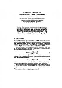
Summing up, the probability distribution P(ε = e|εˆ = t) in Eq. [9], for varying e and fixed t, can be calculated by computer by using the following algorithm. Algorithm PDF_cond: Find Dn, as described in (11). For each pair (u, v) ∈ Dn, calculate the error ε(u, v) using Eq. [7] and the probability P(U = u, V = v|εˆ = t) using either Eq. [10] and Eq. [13] in the stratified case or Eq. [10] and Eq. [14] in the full sampling case. If the error value ε(u, v) has not been encountered before, create a new entry in the probability disˆ = t), othtribution vector and initialize it with P(U = u, V = v|ε ˆ erwise simply add P(U = u, V = v|ε = t) to the existing entry. Results and Discussion Model-Based Results To explain the results and their interpretation, we focus in detail on one case: nonlinear model, ρ = 0.25, LDA classifi-


Confidence Intervals for the True Classification Error cation, and Bayes error 0.15. The six joint distributions of the error and error estimate are given on the companion website. Figure 2(a) gives the marginal distributions of the error estimators using beta fits. The marginal means are shown on the horizontal axis and there we see that leave-one-out cross-validation is essentially unbiased (the red and black diamonds being co-located), 5-fold cross-validation and semibolstered resubstitution are slightly and equivalently highbiased, bootstrap and bolstered resubstitution are slightly low-biased, and resubstitution is greatly low-biased. While the estimated-error mean tells us whether an estimator is globally low-biased or high-biased, it does not tell us the bias of the estimated error conditioned on the true error. The latter is explored in Figure 2(b), where the dotted 45degree line corresponds to the conditional expected estimated error equaling the true error, the estimated-error means are marked on the vertical axis, and the true-error mean is marked on the horizontal axis. We see that for all estimators except resubstitution, if the true error is sufficiently small, then the conditional estimated error is high-biased (curve above the 45-degree line); on the other hand; if the true error is sufficiently large, then the conditional estimated error is low-biased (curve below the 45-degree line). For bolstered resubstitution, which is globally low-biased, the curve falls below the 45-degree line much earlier than the curve for semi-bolstered resubstitution, which is globally high-biased. In sum, across the distributional models being employed (excepting resubstitution), low true errors result in high-biased estimates and high true errors result in low-biased estimates. One of our two main concerns in this paper is the conditional expectation of the true error given the estimated error. The corresponding curves are shown in Figure 2(c), where the estimated-error means are marked on the horizontal axis, and the true-error mean is marked on the vertical axis. Except for resubstitution and bolstered resubstitution, the conditional expected true error varies around the estimated error across the range of the estimate error, the conditional expected true error being larger than the estimated error for small estimated errors and smaller than the estimated error for large estimated errors. The shapes of the curves are revealing. For the high-variance cross-validation estimators, leave-one-out cross-validation and 5-fold crossvalidation, the curves bend more sharply so as to lie beneath the remaining curves as the estimated error increases. This behavior is different than the low-variance bolstered estimators, whose curvatures are much less. The high variation of the cross-validation estimators is evidenced in the extent of their curves to the right. Curves for the conditional variance, Var[ε|εˆ], are shown in Figure 2(d). A high conditional variance means that given a error estimate, the there is large variability in the distribution of the true error.

585

Our second major concern in this paper is the formation of conditional confidence intervals for the true error. Curves for the conditional 95% bounds are shown in Figure 2(e) for the model being considered. As in the case of the conditional expected true error, the means of the estimated errors are marked on the horizontal axis in the figure, but here, besides the red diamond marking the mean true error on the vertical axis, there are also marks giving the mean 95% confidence bounds across all estimated errors. Given an estimated error, a lower bound is better. For most of the estimated error range, and well beyond the mean of the true error, the semi-bolstered resubstitution bound is the best. For very high estimated errors, the cross-validation estimators give the smallest bounds, but looking at the distribution of the true error in Figure 2(a), we see that there is very little mass in this region. What is perhaps most surprising, and not uncommon for other models and classification rules, is the closeness of the mean bounds on the vertical axis. While on average the confidence bound for semi-bolstered resubstitution is slightly lower than the others, there is not much difference, including the mean for the resubstitution bound, which is virtually identical to the means for bootstrap and cross-validation bounds. At first, this might seem remarkable since the confidence-bound curve for resubstitution is so much above the other curves. But we must remember that the mean for the resubstitution estimate is much lower, so that the mass of the resubstitution estimate is concentrated towards the left of the confidence-bound curve, whereas the masses of the other estimates are concentrated much more towards the right of their confidence-bound curves. Finally, in Figure 2(f) we display the deviation distributions for the various estimators using beta fits. We see that the deviation distribution for bolstered resubstitution is very tight, with a bit of low bias and that the distribution for semi-bolstered resubstitution is less tight and a bit high-biased. Bootstrap has less low bias than bolstered resubstitution but significantly higher variance. For this particular feature-label distribution and classification rule, bolstered resubstitution, semi-bolstered resubstitution, and bootstrap perform well among the considered estimators relative to mean deviation, whereas the cross-validation estimators perform poorly owing to their high variances and resubstitution performs poorly owing to its extremely low bias. Error estimation gets better as the sample size increases and we expect to see this reflected in both the conditional expectation and the conditional confidence intervals. Continuing with LDA classification in the nonlinear model, with ρ = 0.25, Bayes error 0.15, and bolstered resubstitution used for error estimation, we have performed the experiments with sample sizes n = 100,150,200,250, the number of repetitions being N = 1,000,000. The conditional expectations and 95% confidence intervals for the true


586

Xu et al.

(a)

0.045

0.45

loo resub cv b632 bresub sresub true error

0.04 0.035

E(estimated error | true error)

Probability density function

0.05

0.03 0.025 0.02 0.015 0.01 0.005 0

(b)

0.4 0.35 0.3 0.25 0.2 0.15 loo resub cv b632 bresub sresub

0.1 0.05

0

0.1

0.2

0.3

0.4

0.5

0.6

0.7

0.8

0.9

1

0.1

0.15

0.2

(c)

0.4 0.35 0.3 0.25 0.2 loo resub cv b632 bresub sresub

0.15 0.1 0

0.35

0.4

0.45

0.5

0.1

0.2

0.3

0.4

0.06 0.055 0.05 0.045 0.04 loo resub cv b632 bresub sresub

0.035 0.03 0

0.5

0.1

0.2

0.3

0.4

0.5

Estimated error

Estimated error 0.08

0.5

(e)

(f)

0.45 0.4 0.35 0.3 0.25 0.2 loo resub cv b632 bresub sresub

0.15 0.1 0

0.1

0.2

0.3

0.4

0.5

Estimated error

Probability density distribution

95% upper-confidence bound for the true error

0.3

0.065 (d)

0.45

Var(true error | estimated error)

E(true error | estimated error)

0.5

0.25

True error

Error

loo resub cv b632 bresub sresub

0.07 0.06 0.05 0.04 0.03 0.02 0.01 0

-0.5

-0.4

-0.3

-0.2

-0.1

0

0.1

0.2

0.3

0.4

0.5

The difference of errors

Figure 2: Nonlinear model, ten correlated features, G = 2, ρ = 0.25, σ2 is set to let the expected Bayes error be 0.15. The markers on the axes show the estimated-error/true-error means or mean confidence bounds.

error given the estimated error for n = 50,100,150,200,250 are shown in Figure 3. In Figure 3(a) we see the conditional expected errors converging on the 45 degree line as n increases and in Figure 3(b) we see a similar phenomenon, where throughout the range of the estimated error the confidence-bound curves are above the 45 degree line and are falling down towards it.

Patient-Data Results Figure 4 shows: (a) the marginal densities of the true and estimated errors; (b) the conditional expectation of the estimated error given the true error; (c) the conditional expectation of the true error given the estimated error; and (d) the 95% confidence interval for the true error given the estimated error.



Confidence Intervals for the True Classification Error

0.5


0.45 0.4 0.35 0.3 0.25 0.2 0.15

n=50 n=100 n=150 n=200 n=250

0.1 0.05 0.05

0.1

0.15

0.2

0.25

0.3

0.35

0.4

Estimated error

587

0.5 0.45 0.4 0.35 0.3 0.25 0.2 0.15

n=50 n=100 n=150 n=200 n=250

0.1 0.05 0.05

0.1

0.15

0.2

0.25

0.3

0.35

0.4

Estimated error

5 4 3 2 1 0.1

0.15

Error

bresub

0.25 0.2 0.15 0.1 0.05 0

0.05

0.1

0.15

0.2

0.25

0.3

0.25

0.3

0.3

0.16

(b)

0.14 0.12 0.1 0.08

bresub

0.06 0.04 0.02 0

0

(d)

0.05

0.1

0.15

True error

0.2

0.25

3 2.5

bresub

0.25

2 1.5

0.2

1 0.5

0.15 0.1

0

(e) BRCA1 BRCA2+sporadic

0 -0.5 -1 -1.5

0.05 0

0.05

0.1

Estimated error

0.15

0.2

0.25

-2

0.3

-3 -2.5 -2 -1.5 -1 -0.5 0

Estimated error

0.5 1

1.5 2

KRT8

0.1

0.2

0.3

0.4

Estimated error

resub, b = 4

0.1

0.2

0.3

0.4

Estimated error

loo, b = 4

resub, b = 8

0.5 0.4 0.3 0.2

0.002 0.004 0.006 0.008 0.010

0.0

95% upper confidence bound for the true error

0.0

Var(true error | estimated error)

Figure 4: Regression analysis with real data.

0.15 0.20 0.25 0.30 0.35 0.40

0

0.2

0.18

DRPLA

0.05

(c)



bresub true error

6

0

0.3

(a)

E(estimated error | true error)

7


Probability density function

Figure 3: The conditional expectations and 95% confidence intervals for the true error given the estimated error for n = 50, 100, 150, 200, 250.

0.0

0.1

0.2

0.3

0.4

Estimated error

loo, b = 8

Figure 5: Conditional error statistics for discrete classification, E[ε] � 0.25, Var[ε] � 0.002. The blue dashed line is the y = x line.


588

Xu et al.

The Linear SVM classifier derived from the patient data (22 samples with seven from BRCA1 and 15 from BRCA2+sporadic) is shown in Figure 4(e). It has bolsteredresubstitution error 0.05. Referring to parts (c) and (d) of Figure 4, the expected true error given the error estimate 0.05 is 0.12 and the 95% confidence bound on the true error given the error estimate 0.05 is 0.20. Exact Performance Results We display exactly computed statistics of the true error given resubstitution and leave-one-out error estimates, under a small sample size and varying the expected true error and number of bins. Owing to the computational complexity of the expressions, we restrict ourselves to n = 20 and a small number of bins. We use a parametric Zipf model, where the parameter controls the difficulty of classification. For simplicity, we will focus here on the stratified sampling case and assume throughout equally-likely classes, i.e., c0 = c1 = 0.5. The Zipf distribution is a well-known power-law discrete distribution, encountered in many applications. The class-conditional probabilities under the parametric Zipf model are given by: pi =

K iα

,

[15]

qi = pb – i + 1,

[16]

for i = 1, 2,…, b. Here α > 0 and the normalizing constant K is given by: K=

b

Σ i=1

() 1 iα

.

[17]

As α → 0, the distributions tend to become uniform, which represents maximum confusion between the classes; whereas, as α → ∞, the distributions become concentrated in single (distinct) bins, which corresponds to maximum discrimination between the classes. In fact, the expected true error of the histogram rule decreases monotonically with α. We consider the case n = 20, under stratified sampling (ten samples of each class) and two values for the complexity, b = 4 and b = 8. In a setting where each feature is binary, this corresponds to classification using two and three features, respectively. For example, in functional genomics, gene expression is often binary (a promoter is either on or off). The cases considered here correspond to prediction using two or three genes, a not uncommon restriction in gene regulatory models. The parameter α in Eqs. [15] through [17] is tuned in both cases (b = 4 and b = 8) to obtain models of low (E[ε] � 0.10), average (E[ε] � 0.25), and high (E[ε] � 0.40) dif-

ficulty [the computation of the unconditional expected error follows the exact method of (11)]. Figure 5 shows the results for the E[ε] � 0.25 case, the results for E[ε] � 0.10 and E[ε] � 0.40 being given on the companion website. The curves for the conditional expectation rise with the estimated error, as with the continuous models. They also exhibit the property that the conditional expected true error is larger than the estimated error for small estimated errors and smaller than the estimated error for large estimated errors. A point to be noted is the flatness of the leave-one-out curves. This reflects the high variance of the leave-one-out estimator. Regarding the 95% confidence bounds, while they are nondecreasing with respect to increasing estimated error, they have flat spots resulting from the discreteness of the estimation rule. This phenomenon is more pronounced when the number of bins is smaller. Concluding Remarks Examining the large array of results presented on the companion website, two general observations are apparent. First, joint behavior between the estimated and true errors, as well as marginal behavior, conditional behavior, and estimation accuracy (behavior of the deviation distributions), is greatly dependent on the feature-label distribution, classification rule, and estimation rule. This observed model sensitivity is in accord with the wide variability in estimation accuracy noted in previous studies. One need only observe the different behavior between linear and polynomial SVM to see the sensitivity to the classification rule. Even more extreme is the behavior of CART. A consequence of this widely varying behavior is that one should use care in choosing a classification rule and error estimation rule. These are not independent and their joint performance depends on the nature of the feature-label distribution. A second key observation is that one must not extend conclusions concerning global estimation properties to local properties. Whereas, one estimation rule might be preferable to another from the perspective of the overall deviation distribution, it might not be preferable for certain ranges of the estimate. The basic point here is that the conditional expected true error, conditional variance of the true error, and the conditional confidence interval are very much dependent on the conditioning value of the error estimate; thereby, making problematic the inferring of local properties from global properties. Although specific results depend on the classification rule, error-estimation rule, and model, some general quantitative trends are seen: (i) if the true error is small (large), then the conditional estimated error is generally high (low)-biased; (ii) the conditional expected true error tends to be larger (smaller) than the estimated error for small (large) estimated errors; and (iii) the confidence bounds tend to be well


Confidence Intervals for the True Classification Error above the estimated error for low error estimates, becoming much less so for large estimates. We emphasize that the particular quantitative nature of the results depends on the parameter Θ governing the feature-label distribution. If one has more or less prior knowledge regarding the feature-label distribution, then this will be reflected in the distribution of Θ and, hence, in the results, in particular, the conditional expectation and conditional confidence bounds. This observation has immediate consequences for application. As we have seen with the patient data, loose specification of the prior distributions can lead to relatively large confidence bounds for small error estimates; nevertheless, prudence demands conservative model postulation. Finally, let us conclude that the results here point in the direction of calibrated error estimation. As is commonplace with measurement devices, rather than apply an error estimator directly, it may be beneficial to calibrate it. Specifically, replace the error estimate with the conditionally expected error given the error estimate. Calibration is problematic because it requires hypotheses on the data. For instance, if we know the feature-label distribution, then the conditional expectation can be found as in the present paper and this can be directly used for calibration. Generally, this is not the case, so that calibration needs to be accomplished using the data in conjunction with assumptions concerning the data. We are currently working on calibration. Acknowledgements This research was supported in part by the National Science Foundation (CCF-0514644) and the Brazilian National Research Council (DCR 35 0382/2004.2). References 1. E. R. Dougherty, A. Datta, and C. Sima. Research Issues in Genomic Signal Processing. IEEE Signal Processing Magazine 22, 46-68 (2005). 2. S. A. Armstrong, J. E. Staunton, L. B. Silverman, R. Pieters, M. L. den Boer, M. D. Minden, S. E. Sallan, E. S. Lander, T. R. Golub, and S. J. Korsmeyer. Mll Translocations Specify a Distinct Gene Expression Profile that Distinguishes a Unique Leukemia. Nat Genet 30, 41-47 (2002).

589

3. I. Hedenfelk, D. Duggan, Y. Chen, M. Radmacher, M. Bittner, R. Simon. P. Meltzer, B. Gusterson, M. Esteller, O. P. Kallioniemi, B. Wilfond, A. Borg, and J. Trent. Gene Expression Profiles in Hereditary Breast Cancer. New England Journal of Medicine 344, 539-548 (2001). 4. L. Li, C. R. Weinberg, T. A. Darden, and L. G. Pedersen. Gene Selection for Sample Classification Based on Gene Expression Data: Study of Sensitivity to Choice of Parameters of the ga/knn Method. Bioinformatics 17, 1131-1142 (2001). 5. J. B. Welsh, P. P. Zarrinkar, L. M. Sapinoso, S. G. Kern, C. A. Behling, B. J. Monk, D. J. Lockhart, R. A. Burger, and G. M. Hampton. Analysis of Gene Expression Profiles in Normal and Neoplastic Ovarian Tissue Samples Identifies Candidate Molecular Markers of Epithelial Ovarian Cancer. Proc Natl Acad Sci USA 98, 1176-1181(2001). 6. M. Bittner, P. Meltzer, Y. Chen, Y. Jiang, I. Seftor, M. Hendrix, M. Radmacher, R. Simon, Z. Yakhini, A. Ben-Dor, N. Sampas, E. R. Dougherty, E. Wang, F. Marincola, C. Gooden, J. Lueders, A. Glatfelter, P. Pollock, J. Carpten, E. Gillanders, D. Leja, K. Dietrich, C. Beaudry, M. Berens, D. Alberts, V. Sondak, N. Hayward, and J. Trent. Molecular Classification of Cutaneous Malignant Melanoma by Gene Expression Profiling. Nature 406, 536-540 (2000). 7. L. Devroye, L. Gyorfi, and G. Lugosi. A Probabilistic Theory of Pattern Recognition. Springer-Verlag, New York, 1996. 8. M. J. van de Vijver, Y. D. He, L. J. van’t Veer, H. Dai, A. A. M. Hart, D. W. Voskuil, G. J. Schreiber, J. L. Peters, C. Roberts, M. J. Marton, M. Parrish, D. Atsma, A. Witteveen, A. Glas, L. Delahaye, T. van der Velde, H. Bartelink, S. Rodenhuis, E. Rutgers, S. Friend, and R. Bernards. A Gene-expression Signature as a Predictor of Survival in Breast Cancer. New England Journal of Medicine 347, 1999-2009 (2002). 9. U. M. Braga-Neto and E. R. Dougherty. Bolstered Error Estimation. Pattern Recogn 37, 1267-1281 (2004). 10. U. M. Braga-Neto and E. R. Dougherty. Is Cross-validation Valid for Small-sample Microarray Classification. Bioinformatics 20, 374380, (2004). 11. U. M. Braga-Neto and E. R. Dougherty. Exact Performance of Error Estimators for Discrete Classifiers. Pattern Recognition 38, 17991814 (2005). 12. C.-C. Chang and C.-J. Lin. LIBSVM: A Library for Support Vector Machines, 2001. Software available at http://www.csie.ntu.edu.tw/~cjlin/libsvm. 13. I. Witten and E. Frank. Data Mining. Academic Press, San Diego, CA. (2000). 14. M. Chernick. Bootstrap Methods: A Practitioner’s Guide. Wily, New York, N.Y. (1999). 15. G. F. Hughes. On the Mean Accuracy of Statistical Pattern Recognizers. IEEE Transactions on Information Theory 14, 55-63 (1968). 16. U. M. Braga-Neto and E. R. Dougherty. Genomic Signal Processing and Statistics, Chapter Classification. EURASIP Book Series on Signal Processing and Communication. Hindawi Publishing Corp. (2005). Received: July 31, 2006; Revised: October 15, 2006; Accepted: October 25, 2006
