the game main tactic. Unfortunately, current games only use scripted and fixed behaviors for their artificial intelligence (AI), and the player can easily learn the ...
Connectionist Reinforcement Learning for Intelligent Unit Micro Management in StarCraft Amirhosein Shantia, Eric Begue, and Marco Wiering (IEEE Member) Abstract—Real Time Strategy Games are one of the most popular game schemes in PC markets and offer a dynamic environment that involves several interacting agents. The core strategies that need to be developed in these games are unit micro management, building order, resource management, and the game main tactic. Unfortunately, current games only use scripted and fixed behaviors for their artificial intelligence (AI), and the player can easily learn the counter measures to defeat the AI. In this paper, we describe a system based on neural networks that controls a set of units of the same type in the popular game StarCraft. Using the neural networks, the units will either choose a unit to attack or evade from the battlefield. The system uses reinforcement learning combined with neural networks using online Sarsa and neural-fitted Sarsa, both with a short term memory reward function. We also present an incremental learning method for training the units for larger scenarios involving more units using trained neural networks on smaller scenarios. Additionally, we developed a novel sensing system to feed the environment data to the neural networks using separate vision grids. The simulation results show superior performance against the human-made AI scripts in StarCraft.
I. I NTRODUCTION
T
HE coordinate behavior of discrete entities in nature and social environments has proved to be an advantageous strategy for solving task allocation problems in very different environments, from business administration to ant behavior [1]. The problem is that only a proper balance of individual decision making (actions) and group coordination (proper time and space allocation of individual actions) may lead a group to perform any task efficiently. Coordination among groups of individual entities using Artificial Intelligence (AI) techniques has been tested on different environments. For example, complex city catastrophe scenarios with limited time and resources in the Robocup Rescue tournaments are a common test place for machine learning techniques applied to achieve cooperative behavior [2], [3]. In addition, video games have gained popularity as common scenarios for implementing (AI) techniques and testing cooperative behavior [4]. The player, an agent, in video games performs actions in a real time stochastic environment, where units controlled by the human or game player have to fulfill a series of finite and clear goals to win the game. Such properties make games an ideal environment to compare machine learning techniques to obtain high quality individual decision making and group coordination behaviors [4]. Amirhosein Shantia and Eric Begue are with the Department of Computer Science, The University of Groningen, The Netherlands (email: {a.shantia}@rug.nl, {ericbeg}@gmail.com) Marco Wiering is with the Department of Artificial Intelligence, The University of Groningen, The Netherlands (email: {M.A.Wiering}@rug.nl)
The relationships between coordination, environmental conditions, and team performance are highly non-linear and extremely complex, leading to an ideal place to establish neural network (NN) based systems. Following this, Polvichai et al., developed an NN system (that was trained with genetic algorithms) which coordinates a team of robots [1]. Their evolved robot teams can work in different domains that users specify and which require tradeoffs. Their evolved neural networks are able to find the best configurations for dealing with those tradeoffs. In games, an NN, that was trained with Neuro-Evolution Through Augmenting Topologies (NEAT), was successfully implemented to improve the cooperation between the ghosts to catch a Pac-man human player in the game [5]. Van der Heijden et al. [6], implemented opponent modeling algorithms (via machine learning techniques) to select dynamic formations in real-time strategic games. However, the game industry is reluctant to use machine learning techniques, because knowledge acquisition and entity coordination with current methods is currently expensive in time and resources. This led to the use of non-adaptive techniques in the AI of the games [4], [5]. A major disadvantage of the non-adaptive approach is that once a weakness is discovered, nothing stops the human player from exploiting the weakness [4]. Even more, the current opponents in AI games are self interested, and because of it, it is difficult to make them cooperate and achieve a coordinated group behavior [5]. Other approaches to coordinate behavior are to use Reinforcement Learning (RL) techniques [7], [8]. RL techniques are implemented in learning tasks when the solution: (i) requires a sequence of actions embedded into deterministic, or more often stochastic environments; and (ii) the system must find an optimal solution based on the feedback from its own actions (generally called the reward). For instance, [9] designed a group of independent decision-making agents with independent rewards based on a Markov game (a framework for RL). Those independent agents have to decide whether they are going to operate on their own, or collaborate and form teams for their mutual benefit when the scenario demands it. The results show a performance improvement in environments with restriction on communication and observation range. In addition, Aghazadeh et al., developed a method called Parametric Reinforcement Learning [10], where the central part of the algorithm is to optimize, in real time, the action selection policies of different kinds of individual entities with a global and unique reward function. Their system won the city-catastrophe scenario in the Robocup Rescue tournament in 2007 which proves the efficiency [10]. A proper method for video-game AI must fit and learn
the opponent behavior in a relatively realistic and complex game environment, with typically little time for optimization and often with partial observability of the environment [4], [5]. It has been shown that neural networks are very efficient methods for approximating a complicated mapping between inputs and outputs or actions [11], [9], [10], and therefore we will also use them in our research. The Neural-Fitted Q-iteration (NFQ-i) algorithm was developed to exploit the advantages of a neural network to approximate the value function, and RL techniques to assign credit to individual actions [12]. In some applications NFQ-i has been shown to be much more experience efficient than online RL techniques. These properties predict that NFQ-i can be a powerful tool for learning video-game AI. In this paper, we developed the Neural-Fitted Sarsa (NFS) algorithm and compare it to online Sarsa [13], [14] on a simulation using StarCraft, in which efficient game strategies should be learned for a team of fighting units. StarCraft is one of the most popular real-time strategic games, and it has complex scripted AI which makes it an ideal candidate to prove the efficiency of the NFS technique. Real time strategy games are not only an interesting topic for sole research purposes. The video game industry has roughly sold eleven billion dollars in 2008 and 2009. The share for PC games are around seven hundred million dollars. Real time strategy games dominate the PC games sell by 35.5%. Therefore, any breakthrough in this field is a potential investment for financial success [15]. The university of Santa Cruz held a competition in 2010 (AAID 2010) in which StarCraft micro-management was one of the tournaments. The winner of that tournament used a finite state machine to control units. Our method, on the other hand, uses reinforcement learning algorithm with neural networks which can adapt themselves to changing enemy tactics and can find new tactics based on the team’s experiences without supervision [16]. Contributions. In this paper we explore whether connectionist reinforcement learning techniques can be useful for obtaining good performing game AI for controlling a set of units in a battlefield scenario in the game StarCraft. First of all, we compare neural-fitted Sarsa to online Sarsa to see whether the neural-fitted approach can better exploit limited experiences for obtaining good quality AI. Next, we introduce vision grids for obtaining terrain information about the dynamic state of the battlefield. Furthermore, we propose an incremental learning approach where the action-selection policies for larger teams are pretrained using the experiences obtained by smaller teams. This incremental learning is then compared to training bigger teams with randomly initialized neural networks. It is important also to note that, unlike the standard scripts or limited finite state machines where the design is bound to the type of units, our proposed methods can adapt themselves automatically against different types of enemies in different terrains. Therefore, if our system is successful it could be very applicable to learn to produce game AI for this game genre.
���� � ������������ ��� �� � �� ��� ������ � �� ������ ����� � � ���� �� � ����������� ������ ������ ����� � ������ ������ ����� � ������ �������� � ������ ��� ������ � ���� ������ �� ��� � � ���� �� ������� ���������
��� ������ � ����������������
���
�� ��
��
��
� ������ ����� � ! ����"������ ������� � ! ����"������ ��� ������ � ! ����"������ ������ �������
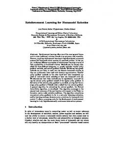
Fig. 1. The game state information (agent internal state and environment) are fed to a Neural Network with one hidden layer and one output unit that represents the Q-value.
Outline. In the next section, we first describe the game StarCraft, and then our proposed neural network architecture. We will there also describe the game environment and our vision grids. In Section III, we present our proposed reinforcement learning techniques. In Section IV, we show the results of 6 experiments where our learning systems train different sized teams to fight against the prescripted game AI used in StarCraft. Section V concludes this paper. II. S TAR C RAFT A. StarCraft
AND
N EURAL N ETWORKS
TM
StarCraft TM is a popular Real-Time War Strategy (RTS) video game developed by Blizzard Entertainment in 1998. StarCraft is the most successful RTS game with more than 9.5 million copies sold from its released date in 1998 until 2004. StarCraft consists of three races and involves building structures and using different types of soldiers to engage in battle. The game-play in these games involves unit micromanagement, building order, resource management, and the game main tactic. In this paper we focused on micromanagement of a number of units with the same type. The game has a terrain with different possible heights, choke points, etc. Each unit of the game has a number of attributes such as health, armor, weapon, move speed, attack speed, turn speed, etc. Player unit information is always accessible to the player, but enemy unit information can be chosen to be visible or hidden when it is out of sight. We currently use global knowledge to simplify the problem and avoid training an exploration technique, which would be necessary if the opponent cannot be seen otherwise. B. Neural Networks As mentioned before, the game environment contains a lot of information such as player and enemy locations, self attributes and a number of actions that each unit can perform. The relationship between the possible actions and the state of the game is non-linear and involves a high number of dimensions, leading to an ideal place to establish a neural network approach (Figure 1). We use several multi-layer NNs to approximate the state-action value function Q(st , at ) that denotes the expected future reward intake when performing action at in state st at time t. As activation function for the hidden layer, we used the hyperbolic tangent, and a
linear activation function for the output unit. Following the research described in [17] each NN is dedicated to one action-type. The input units represent the state and the output represents the Q-value for the action corresponding to the neural network. We used a feedforward multi-layer perceptron with one hidden layer. It can be described as a directed graph in which each node (i) performs a transfer function fi formalized as: n X ωij xj − θi ) yi = fi (
(1)
j=1
Where ωij are the weights and θi is the bias of the neuron. After propagating the inputs xj forward through the neural network, the output of the NN represents the Qvalue for performing a specific action given the state of the environment. 1) Environment and Input: We feed the neural networks with information we consider important to evaluate the game state (see Figure 1). This information constitutes our learning bias. The data sent to the neural networks are relative to the agent and are classified into two categories, which are: 1) Agent Internal State a) Hit points b) Weapon status c) Euclidean distance to target d) Is target the same as previous? 2) Environment State (Ally and Enemy) a) Number of Allies targeting this enemy b) Number of enemies targeting current unit c) Hit points of Allies and Enemies d) Surrounding environment dangerousness The variables in this last category are collected using ally and target state and different vision grids (see Section II-B3). The agents use this information to select an action one by one. 2) Input value normalization: Every input variable from the game-state is normalized before it is processed by the NNs. The variables that have an intrinsic maximum value (e.g. hit points) are normalized in a straightforward way, that is by x/xmax . The other variables that do not have an obvious maximum value are expressed as a fraction of a constant. For example, the number of units are expressed as a fraction of the number of units alive at the beginning of each game round, and distances are expressed as a fraction of the length of the entire map. 3) Vision Grids: In a battlefield scenario, terrain information is essential for the performance of a team. Terrain information contains clues or measurements about the battle field configuration. It is very time consuming to consider all the information in the environment at once for decision making. Therefore, we divided decision making into two phases. First, when the units are far, decisions are only made by simple hit point and damage calculation. Next, when they are close the neural networks for the computer players can take into account all the information around a unit. To encode this kind of information we use a grid
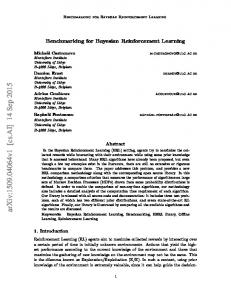
Fig. 2. Illustration of the usage of a vision grid to collect information about the dangerousness.
data structure. Our approach uses several small grids, where each encodes a specific type of battle field information such as location, weapon state, hit points, weapon cool downs, weapon range, etc. Currently, 9 different grids are used, each of which carries information about enemy and ally locations and hit points, targets of allies and enemies, the position of the current target being evaluated, dangerousness of surrounding locations, and finally the supported positions for the current unit. For example, the dangerousness grid is a map that tells how much it is dangerous or safe for a unit being at a specific location based on the attacking range and power of the enemies relative to that location, see Figure 2. A grid is centered on the agent and oriented accordingly with the facing direction of the agent (direction invariant). Each grid cell is either zero (if no information is present regarding that specific grid cell) or a number which gives specific information related to that cell. The grid information will finally be reshaped to a vector and will be added to the neural network input. Figure 2 illustrates the usage of grids to collect information about the dangerousness around the learning agent. The learning agent is represented as a red dot and its facing direction is denoted by the little arrow. Similarly, two enemies are represented in blue. The attack range of each enemy is drawn using the large circles. A vision grid is centered at the agent’s position and oriented in its facing direction. The numbers in the cells represent the dangerousness at the cell position, the value here represents the hypothetic fraction of the total hit points a unit can lose when being attacked at the corresponding location. Those values are for illustrative purpose and do not correspond to the actual game. The cells
with zero value are left blank. Notice that the dangerousness is higher at locations attackable by both enemies. Each cell is a neural network input unit. The proposed method has a number of advantages. Since the evaluation is done for each pair of units, an infinite number of units can use the architecture and, because the grids are rotation invariant, the number of learning patterns are limited. III. R EINFORCEMENT L EARNING When a task requires a sequence of actions to be done by an agent in a dynamic environment, one of the most common methods to make the agent to learn improving its behavior is reinforcement learning (RL) [7], [8]. The agent will start choosing actions depending on the state of the game by using the neural networks to output a single value for each action. An action will be selected based on the Q-values and an exploration strategy to deal with the exploitation/exploration dilemma [18]. When the action is done, a reward will be given to the action which is the feedback of the environment to the agent. After the final state of the game is reached, which in our case is the end of a single game round (after one of the two teams lost all its soldiers), the state-action value functions corresponding to the neural networks will be updated depending on state transitions and the rewards received during the game. Finally, the computed target values are back propagated through the neural network to update the weights. The agents should predict the state-action value, Q(st , at ), for each state st and each possible action at . This value reflects the predicted future reward intake after performing the action in that specific state, and the optimal Q-values should obey the Bellman optimality equation given by: Q∗ (st , at ) = E[rt ] + γ
X st+1
P (st+1 |st , at ) max Q∗ (st+1 , a) a
(2) Where P (st+1 |st , at ) denotes the state-transition function, E[rt ] the expected reward on the transition, and a discount factor 0 ≤ γ < 1 is used to discount rewards obtained later in the game. When γ is close to one, the agent is far-sighted and the rewards received in the future count more. On the other hand, when γ is zero, only the immediately obtained reward counts. A. Online Sarsa and Boltzmann exploration The most widely known online value-function based reinforcement learning algorithms are Q-learning [19], [20] and Sarsa [13], [14]. In preliminary experiments, our results indicated that Sarsa performed better for training the StarCraft fighting units than Q-learning. Therefore all our reported experiments use Sarsa as reinforcement learning technique. Sarsa is an on-policy method, which means that the policy is used both for selecting actions and for updating previous action Q-values. The online Sarsa update rule is shown in equation 3. Q(st , at ) ← Q(st , at ) + α[rt + γQ(st+1 , at+1 ) − Q(st , at )] (3)
The Boltzmann exploration strategy uses the Q-values to select actions in the following way: eQ(st ,a)/τ P (a) = P Q(s ,b)/τ t be
(4)
Here τ denotes the temperature, which we will decrease progressively in our experiments according to a cooling schedule. The computed action-probabilities P (a) are then used to select one final action. B. Actions In our system for training the StarCraft AI, we used two action types for all the agents. The units can either target an enemy and approach and attack them or they can evade from the battlefield. To calculate the evade location we consider the direct line between enemies and the current unit and the weapon range. Next, we take the average of these vectors and the opposite location of it will be selected. If the evade action is selected, the unit will move away from enemies until it reaches a safe spot. However, when a unit is surrounded, it will remain in its position. For the attack action, for each ally unit, all the enemy units will be evaluated using the inputs mentioned in the previous section. After a decision is made, units have a limited amount of time to perform the action. If the limit is passed, the action is canceled and another action will be selected. Each type of action is associated with a unique neural network. To evaluate a specific action, the neural network associated with the action type is fed with the inputs describing the state of the game, the neural network is activated and its output is the action Q-value. At each time-step an action needs to be selected, a living unit will compute with one neural network the Q-value for the evade action, and with another neural network the Q-value for attacking each enemy unit. Since information about the enemy unit is given as input to the neural network, in this way we can deal with an arbitrary amount of units, while still only having to train two neural networks. Finally, it is important to note that we used policy sharing in our system, which means that all units use the same neural networks and all the experiences of all units are used to train the neural networks. C. Dealing with Continuous Time RL techniques are well defined and work well with discrete time-steps. In StarCraft, the state (internal variables) of the game is updated in each frame, that is approximately twenty five times per second when the game is running at the normal playing speed. This update speed contributes to the real time aspect of the game. Despite the fact that the frame by frame update is discrete, the change of the game state is better conceived as being continuous when observed at the round time scale, that is at a scale of the order of seconds. In order to apply RL to this game we have to somehow discretize the continuous time. The first approach we had was to consider that a new state occurs after a number of frames (e.g. 25 frames, or one real second) have elapsed.
We encountered several problems with this approach. To illustrate an important one, it may happen that the agent is unable to perform a selected action, because it is busy doing a previous action and thus can not be interrupted. In this situation, the reward for a specific action may not be adequately given, resulting in a noisy reward. The second and last approach we used was more appropriate regarding applying RL to this dynamic game. We consider that a new state occurs when the agent has finished performing an action. So one step is as follow: the agent observes the state at time t, selects an action to perform from a set of possible actions, performs the selected action while the game is continuously updating (the clock is ticking), and after the action is done, the game is in a new state at time-step t + 1, and the agent uses its obtained reward in that interval to update its Q-function. D. Reward Function The performance of RL techniques may depend heavily on the reward function, which must sometimes be carefully designed to reflect the objectives of the task. Because the objective of the player in real time strategic games is to defeat the enemy in the battle, we designed a reward function that reflects this properly. Ally’s total hit points, number of alive allies, enemy total hit points, and number of alive enemies are the properties to measure this reward. The reward Ri for a frame i is given to each agent after it has done an action, and is computed using: Ri = damageDone−damageReceived+60∗numberKills (5) Where numberKills only uses the number of killed opponents during a frame. 1) Short Term Memory Reward Function: Using the previous reward function, that indicates the reward per frame, we developed a Short Term Memory Reward (STMR) function that computes a cumulative reward on a continuous basis. When an event occurs in which a reward is emitted (positive or negative), the value of the temporary reward-sum increases or decreases accordingly. When time passes, the absolute value of the total reward of all frames during performing the same action decreases by a decaying factor κ, which makes the reward decay in time. The agent receives the reward when an action is done at the next frame, which corresponds to a transition to the next time-step t + 1. The reward at time t (rt ) at the f th frame after starting executing the action is computed as follows: X Ri κf −i , rt = i
where Ri is the reward at frame i and κ is the decaying factor. This method is a bit similar to the use of macroactions, options, etc. in the Semi-Markov decision process framework, but an important difference is that in our shortterm reward function the rewards closest to the end of the action are more important. Furthermore, the number of timesteps are not used to discount the next state-action pair’s
Q-value in the update rule. We have also done experiments with the standard use of Semi-Markov Decision Processes, but our above described method performed much better. 2) Dead Units: Another problem that we faced during training was distributing the correct reward when an ally or enemy unit is dead. Normally, at the end of the game we give positive or negative reward values to all the units if they won or lost the game respectively. However, assigning rewards and punishments to units that die during a game round is not an easy problem. Consider a case when the team is winning but a unit dies in the process. Possibly the unit’s decisions were perfect, but it was the enemy’s focus that killed the unit. Therefore, it is not correct nor fair to just give a negative reward (we did not achieve good results by punishing dead units). Consequently, the reward of a dead unit during the game is the average reward of all living units in the next state. This makes sure that even the dead units will receive positive rewards when the team is acting well. However, when an enemy unit is killed, it is not fair to distribute the same amount of reward to all the units. Therefore, the unit with the highest kill count will receive the highest reward. This means that all units optimize their own different reward intake. Although the units are self-interested agents, the reward function is selected in such a way, that they all profit from a cooperative behavior in which they together defeat the opponent team. Algorithm 1: Neural-Fitted Sarsa algorithm pseudo-code NFS main () input a set of transition samples D, an MLP; output: Updated MLP that represents QN k=0 while k < N do Generate Pattern set P = {(inputl , targetl ), l = 1, ..., #D}, Where: inputl = sl , al targetl = rl + γQk (sl+1 , al+1 ) MLP-training(P ) → Qk+1 k := k + 1 end while
E. Neural-Fitted Sarsa We also compare online Sarsa to Neural-Fitted Sarsa (NFS). Neural-Fitted Sarsa is heavily inspired by the success of neural-fitted Q-iteration [12], and we want to test if it is a promising technique for training StarCraft teams. Neuralfitted techniques rely on neural networks that are trained multiple times on a large set of training experiences. The problem with online reinforcement learning methods and neural networks is that learning is slow. Instead of updating the Q-values online with Sarsa, we can also use the NeuralFitted Sarsa method in which the updates are done off-line considering an entire set of transition experiences collected in quadruples (s, a, r, s′ ). Here s is the initial state, a is the chosen action, r is the reward, and s′ is the next
TABLE I L EARNING PARAMETERS FOR NFS AND O NLINE S ARSA .
1
0.9
STMR (0.8 decay) 0.5 0.001 671 0.51 0.995 50 9×9
0.8
0.7
Winning Ratio
Reward Function Discount Rate Learning Rate Number of inputs Temperature start Temperature drop NN Hidden Units NN Vision Grid size
0.6
0.5
0.4
0.3
0.2
state. The method allows the establishment of a supervised learning technique for the NN that may lead to more efficient experience use as shown in [12]. The pseudo-code of NFS is given in Algorithm 1. We use N = 5 in our experiments, so that the experiences are replayed 5 times to update the MLP.
0.1
0
1
2
3 Game Rounds
4
5
6 4
x 10
(a) Online Sarsa 1
F. Incremental Learning
0.9
AND
0.8
0.7
Winning Ratio
The number of game states in scenarios involving a large amount of units (e.g. 6 vs. 6) is very large. Therefore, it may take a prohibitive amount of learning time to learn the right team strategies. The idea of using incremental learning is to first train the neural networks with RL techniques on a smaller problem involving less units and therefore less game states. Then, after pretraining the neural networks in this way, they can be used as a start to learn on larger scenarios. A problem that has to be dealt with in this approach is that the larger scenarios also involve more inputs, since in general information about each ally and enemy unit is passed to the neural networks. To cope with this, we use neural networks with as many inputs needed to deal with the larger scenario, and when learning on the smaller scenario always set the additional input units to the value 0. In this way we can simply reuse the trained neural networks, and after that they can learn to make use of the newly available inputs. IV. E XPERIMENTS
0
0.6
0.5
0.4
0.3
0.2
0.1
0
0
1
2
3 Game Rounds
4
5
6 4
x 10
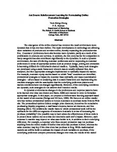
(b) NFS Fig. 3. The winning ratio versus game rounds of a three versus three marines scenario. The comparison of online Sarsa versus neural fitted Sarsa. The blue line is the mean and the red lines are 68% confidence intervals. After each 500 games the average number of times the RL systems won against the standard human-made StarCraft team is plotted.
R ESULTS
As mentioned before, the simulation environment is the StarCraft game engine. We focused our experiments on unit micro management where a balanced number of units of the same type will fight against each other. The simulations were done in three versus three and six versus six scenarios. The units are marines that can attack a single unit with ranged weapons. In this section we show the results of 6 experiments. First, we compare online Sarsa to the Neuralfitted Sarsa method using the STMR reward function on a 3 vs. 3 battlefield scenario. Next, we compare the learning performance on a more difficult 6 vs. 6 scenario. Finally, we compare the results with an incremental learning approach on the 6 vs. 6 scenario. The incremental scenario uses the previously trained neural networks in the 3 vs. 3 case as a start for training in the 6 vs. 6 scenario. In non-incremental learning, we start the training procedure with a randomly initialized neural network. A. NFS vs. Online Sarsa We first compare the NFS algorithm to the online Sarsa algorithm. The first experiment involves a three versus three
learning scenario in which we start with NNs that are initialized with random weights. In the NFS system the NNs are updated after every (50) game rounds, while in the online method, the NNs are updated after each game round. The temperature used by Boltzmann exploration drops after every 100 game rounds for both methods. The learning parameters of both systems, except the update methods, are the same. These parameters are presented in Table I. For these simulations, we run the scenarios for 50,000 to 60,000 game rounds, which lasts approximately 12 hours with the game running at full speed. For each method we repeated the experiment 5 times with different random seeds and calculated the mean and standard deviations. As can be seen in Figure 3, both methods converge to a similar solution of around 72% average winning ratio. Thus, both methods are able to learn to significantly outperform the standard StarCraft game AI. The figure also shows that the online method unexpectedly learns faster than the neuralfitted method, although when we give the NFS method a bit more training time (60,000 game rounds), it is able to obtain
1
0.9
0.9
0.8
0.8
0.7
0.7
0.6
0.6
Winning Ratio
Winning Ratio
1
0.5
0.5
0.4
0.4
0.3
0.3
0.2
0.2
0.1
0.1
0
0
1
2
3 Game Rounds
4
5
0
6
0
1
1
1
0.9
0.9
0.8
0.8
0.7
0.7
0.6
0.6
0.5
0.4
0.3
0.3
0.2
0.2
0.1
0.1
1
2
3 Game Rounds
4
5
6 4
x 10
0.5
0.4
0
3 Game Rounds
(a) Online Sarsa
Winning Ratio
Winning Ratio
(a) Online Sarsa
0
2
4
x 10
4
5
6 4
x 10
0
0
1
2
3 Game Rounds
4
5
6 4
x 10
(b) NFS
(b) NFS
Fig. 4. The winning ratio versus game rounds of non-incremental six versus six marines scenario. The comparison of online Sarsa versus neuralfitted Sarsa. The blue line is the mean and the red lines are 68% confidence intervals.
Fig. 5. The winning ratio versus game rounds of incremental six versus six marines scenario. The comparison of online Sarsa versus neural-fitted Sarsa. The blue line is the mean and the red lines are 68% confidence intervals.
the same level of performance as online Sarsa. We also compared the same methods in a six versus six learning scenario. We randomized weights and then let the system train the 6 soldiers. It should be mentioned that the number of possible patterns in a 6 vs. 6 scenario is much larger than in the 3 vs. 3 scenario. As can be seen in Figure 4 both methods are performing much weaker than in the 3 vs. 3 scenario, and are unable to defeat the StarCraft game AI. The online Sarsa system seems to achieve a better performance than the neural-fitted Sarsa algorithm. B. Incremental vs. Non Incremental Learning We saw that by going from a three versus three scenario to a six versus six scenario, learning became much harder. However, as described in Section III, we can use the trained neural networks on the 3 vs. 3 scenario as a start for further training on the 6 vs. 6 scenario. Figure 5 shows the results with this incremental approach for both online Sarsa and neural-fitted Sarsa. The figure clearly shows that the performance with incremental learning is much better than without incremental learning. Table II shows the average winning ratio and the best winning ratio
of the learned game AI against the handcrafted StarCraft AI. It shows that the learned behaviors are able to outperform the StarCraft AI, although not all learning runs result in the same good behavior. In the 3 vs. 3 scenario, the best results of 85% winning are obtained with the NFS method, whereas in the 6 vs. 6 scenario the best results of 76% winning are obtained with online Sarsa that uses incremental learning. The Table clearly shows the importance of incremental learning to obtain good results in the complex 6 vs. 6 scenario. V. C ONCLUSION In this paper, we presented a reinforcement learning approach to learn to control fighting units in the game StarCraft. StarCraft is one of the most famous real time strategy games developed unit now, and has recently been used in tournaments to compare the use of different techniques from artificial intelligence. We compared online Sarsa to neuralfitted Sarsa, and the results showed no clear improvement by using a neural-fitted approach. This may be because there are lots of different game patterns, and each new game follows different dynamics, so that only a small bit can be learned from each game. The results also showed that the
TABLE II T HE RESULT OF ALL SIMULATIONS . T HE TABLE SHOWS THE WINNING RATIOS OF THE LAST 1000 GAMES PLAYED . 3 3 6 6 6 6
vs. vs. vs. vs. vs. vs.
3 3 6 6 6 6
Online Sarsa NFS Online Sarsa NFS Incremental Online Sarsa Incremental NFS
Average Winning Ratio 70% 75% 35% 22% 49% 42%
proposed methods were very efficient for learning in a 3 vs. 3 scenario, but had significant problems to learn in a larger 6 vs. 6 soldier scenario. To scale-up the proposed RL techniques, we proposed an incremental learning method, and the results showed that using incremental learning, the system was indeed able to defeat the scripted StarCraft game AI in the complex 6 vs. 6 soldier scenario. In future work, we want to research extensions with learning team formations, which may be essential to scale up to even larger teams. This will involve learning to create subgroups of soldiers, but also the patterns with which they approach the enemy units. Furthermore, we want to study better exploration methods to find critical states in the environment. R EFERENCES [1] J. Polvichai, M. Lewis, P. Scerri, and K. Sycara, Using Dynamic Neural Network to Model Team Performance for Coordination Algorithm Configuration and Reconfiguration of Large Multi-Agent Teams, C. H. Dagli, A. L. Buczak, D. L. Enke, M. Embrechts, and O. Ersoy, Eds. New York, NY: ASME Press, 2006. [2] M. R. Khojasteh and A. Kazimi, “Agent Coordination and Disaster Prediction in Persia 2007, A RoboCup Rescue Simulation Team based on Learning Automata,” in Proceedings of the World Congress on Engineering 2010 Vol I., ser. WCE 2010. Lecture Notes in Engineering and Computer Science, 2010, pp. 122–127. [3] I. Martinez, D. Ojeda, and E. Zamora, “Ambulance decision support using evolutionary reinforcement learning in robocup rescue simulation league,” in RoboCup 2006: Robot Soccer World Cup X, ser. Lecture Notes in Computer Science, G. Lakemeyer, E. Sklar, D. Sorrenti, and T. Takahashi, Eds. Springer Berlin / Heidelberg, 2007, vol. 4434, pp. 556–563. [4] S. C. Bakkes, P. H. Spronck, and H. J. van den Herik, “Opponent modelling for case-based adaptive game AI,” Entertainment Computing, vol. 1, no. 1, pp. 27 – 37, 2009. [5] M. Wittkamp, L. Barone, and P. Hingston, “Using NEAT for continuous adaptation and teamwork formation in pacman,” in Computational Intelligence and Games, 2008. CIG 2008. IEEE Symposium On, december 2008, pp. 234 –242.
Standard Deviation 10% 11% 5% 7% 28% 27%
Best Winning Ratio 80% 85% 36% 24% 76% 61%
[6] M. van der Heijden, S. Bakkes, and P. Spronck, “Dynamic formations in real-time strategy games,” in Computational Intelligence and Games, 2008. CIG ’08. IEEE Symposium On, december 2008, pp. 47 –54. [7] L. P. Kaelbling, M. L. Littman, and A. W. Moore, “Reinforcement learning: A survey,” Journal of Artificial Intelligence Research, vol. 4, pp. 237–285, 1996. [8] R. S. Sutton and A. G. Barto, Reinforcement Learning: An Introduction. The MIT press, Cambridge MA, A Bradford Book, 1998. [9] A. C. Chapman, R. A. Micillo, R. Kota, and N. R. Jennings, “Decentralised dynamic task allocation: a practical game: theoretic approach,” in Proceedings of The 8th International Conference on Autonomous Agents and Multiagent Systems - Volume 2, ser. AAMAS ’09. Richland, SC: International Foundation for Autonomous Agents and Multiagent Systems, 2009, pp. 915–922. [10] O. Aghazadeh, M. Sharbafi, and A. Haghighat, “Implementing parametric reinforcement learning in robocup rescue simulation,” in RoboCup 2007: Robot Soccer World Cup XI, ser. Lecture Notes in Computer Science, U. Visser, F. Ribeiro, T. Ohashi, and F. Dellaert, Eds. Springer Berlin / Heidelberg, 2008, vol. 5001, pp. 409–416. [11] E. Alpaydin, Introduction to Machine Learning. The MIT Press, 2004. [12] M. Riedmiller, “Neural fitted Q iteration: first experiences with a data efficient neural reinforcement learning method,” in 16th European Conference on Machine Learning. Springer, 2005, pp. 317–328. [13] G. Rummery and M. Niranjan, “On-line Q-learning using connectionist sytems,” Cambridge University, UK, Tech. Rep. CUED/F-INFENGTR 166, 1994. [14] R. S. Sutton, “Generalization in reinforcement learning: Successful examples using sparse coarse coding,” in Advances in Neural Information Processing Systems 8, D. S. Touretzky, M. C. Mozer, and M. E. Hasselmo, Eds. MIT Press, Cambridge MA, 1996, pp. 1038–1045. [15] ESA, “Essential facts about the computer and video game industry,” 2010. [16] U. of Santa Cruz, “StarCraft AI Competition,” http://eis.ucsc.edu/ StarCraftAICompetition, 2010, [Online]. [17] L.-J. Lin, “Reinforcement learning for robots using neural networks,” Ph.D. dissertation, Carnegie Mellon University, Pittsburgh, January 1993. [18] S. Thrun, “Efficient exploration in reinforcement learning,” CarnegieMellon University, Tech. Rep. CMU-CS-92-102, January 1992. [19] C. J. C. H. Watkins, “Learning from delayed rewards,” Ph.D. dissertation, King’s College, Cambridge, England, 1989. [20] C. J. C. H. Watkins and P. Dayan, “Q-learning,” Machine Learning, vol. 8, pp. 279–292, 1992.