CONTEMPORARY VIEW OF FFT ALGORITHMS Aravind Ganapathiraju, Jonathan Hamaker, Joseph Picone
Anthony Skjellum
Institute for Signal and Information Processing Department of Electrical and Computer Engineering Mississippi State University, Mississippi State, MS-39762 {ganapath, hamaker, picone}@isip.msstate.edu
High Performance Computation Laboratory Department of Computer Science Mississippi State University, Mississippi State, MS-39762
[email protected]
ABSTRACT A large number of fast Fourier transform (FFT) algorithms exist for efficient computation of the discrete Fourier transform (DFT). In most previous benchmarking efforts, only the computation speed or the operations count have been used for assessing the efficiency of these algorithms. In this paper we provide a comprehensive comparison of several contemporary FFT algorithms on state-of-the-art processors. The criterion used are the operations count, CPU time, memory usage, processor, and compiler. The processors that were evaluated include the DEC Alpha, Intel Pentium Pro and Sun UltraSparc. Preliminary work on quantifying the effects of compilers on these algorithms is also presented. The most efficient algorithm was found to be the fast Hartley transform. For some algorithms, the results presented here differ significantly from theoretical predictions, thereby stressing the need for such contemporary benchmarks.
1. INTRODUCTION A large number of FFT algorithms have been developed over the years for the efficient computation of the DFT. The first major breakthrough was the Cooley-Tukey algorithm [1] developed in the mid-sixties which resulted in a flurry of activity on FFTs. This algorithm reduced the 2
have been compared based on their floating point operation counts), there has been little research to-date comparing algorithms on practical terms. The choice of the best algorithm for a given platform is still not easy because efficiency is intricately related to how an algorithm can be implemented on a given architecture. The important issues to be considered in comparisons are the computation speed, memory, algorithm complexity, machine architecture and compiler design. Therefore, we present what we believe to be the most recent comprehensive benchmarking of a few commonly used algorithms on widely available high-speed state-of-the-art CPUs. In this paper we provide the results of this benchmarking process on 6 different algorithms. These results will help correlate the numbers predicted by theory with the actual measured values. The CPUs used in this comparison are the DEC Alpha, Intel Pentium Pro and Sun UltraSparc. To quantify the effect compilers have o n algorithm performance, we have evaluated the Microsoft Visual C++ compiler and GCC, a publicly available compiler.
2. ALGORITHMS Most FFT algorithms achieve their speedup by computing an N-order DFT through successive computations of lower order DFTs.
complexity of a DFT from O( N ) to O(NlogN), which at the time was a tremendous improvement in efficiency. Algorithms which followed have achieved this complexity reduction to varying degrees. The Cooley-Tukey algorithm was a Radix-2 algorithm [8,9]. The next few radix algorithms developed were the Radix-3, Radix-4, and the Mixed Radix algorithm. Further research led to the Fast Hartley Transform (FHT) [2,3,4,10] and the Split Radix (SRFFT) [5,9,10] algorithm. Recently, two new algorithms have also emerged: the Quick Fourier Transform (QFT) [6] and the Decimation-in-Time-Frequency (DITF) [7].
Standard radix-2 (RAD2) algorithms are based on the synthesis of two half-length DFTs[1,8,9]. Radix-4(RAD4) algorithms are based on the synthesis of four quarter-length DFTs[1,8,9]. The Split-Radix algorithm is based on the synthesis of one half-length DFT together with two quarterlength DFTs[1,8,9]. This works because the radix-2 algorithm computes the even numbered samples independently of the odd numbered points. Therefore, the split-radix algorithm uses the radix-4 algorithm to compute the odd numbered DFT coefficients and the radix-2 to compute the even DFT coefficients.
While there has been extensive research on the theoretical efficiency of these algorithms (traditionally algorithms
The FHT evolved out of applying the same strategies used for the radix-based FFT algorithms for the computation of
Computation Time (log scale)
5.0
RAD2 algorithm, most of the computations (especially complex multiplications) are done in the initial stages of the algorithm. However, in the Decimation-in-Time (DIT) implementation of the RAD2 algorithm, most of the computations are done in the final stages of the algorithm. Thus, a straightforward approach to increase efficiency is to start with the DIT implementation and then shift to a DIF implementation at some later stage.
DEC Alpha 300MHz Pentium Pro 200MHz UltraSparc 200MHz
4.5
4.0 3.5 3.0 2.5
3. EXPERIMENTS AND RESULTS 1024
4096
16384
FFT Order Figure 1. Computation speed across machines the discrete Hartley transform. The main difference between the other algorithms discussed here and the hartley transform is the core kernel which is real, of the form jω
cos θ + sin θ , unlike the complex exponential ( e )for the DFT. Thus, the FHT is intuitively simpler and faster since the number of computations reduces drastically when we remove all complex computations. Similar to the other recursive radix algorithms, the higher order FHTs can be obtained by combining lower order FHTs. In the QFT algorithm the symmetry properties of the cosine and the sine functions are exploited to derive an efficient algorithm. The N-point DFT computation is achieved via a (N/2+1)-point discrete cosine transform (DCT) and a (N/2-1)-point discrete sine transform (DST). Since complex operations occur only in the last stage of the computation where the DCT and DST are combined, the QFT is expected to perform efficiently on real data. The DITF algorithm is based on the observation that, in a Decimation-in-Frequency (DIF) implementation of a FFT Order Algorithm 64
256
1024
4096
16384
RAD2
60
280
1960
10900
97100
RAD4
60
250
1800
9720
58220
SRFFT
40
160
1060
6140
38100
FHT
40
140
640
3800
38100
QFT
40
160
880
6560
44020
DITF
60
360
2500
12320
104080
Table 1: Performance across different FFT orders when run on an UltraSparc2
After implementing each of these algorithms in a common framework, we comprehensively benchmarked these algorithms. In the process we observed several results that were contrary to published theory. Many of these surprises can be attributed to compiler optimizations rather than discrepancies in the algorithms or the measurement process. Some algorithm implementations tend to be more amenable to optimizations on modern processors than others. In implementing the algorithms, we have tried to use uniform techniques for operations such as bit-reversal and lookup table generation so that the difference we see in performance can be attributed solely to the efficiency alone. 3.1. Computation Speed In most present day applications computation speed is by far the most important aspect of an algorithm one is interested in. Not only can we benchmark algorithms in terms of computation speed, but we can also benchmark processors using the same criteria. It is interesting to see how the performance of the algorithms scales in terms of processor speed. This is very heavily influenced by the architecture, cache usage, and other hardware-related features as illustrated in Figure 1. We evaluated each of the algorithms using the same compiler (GCC version 2.7.2.1) on a 200 MHz PentiumPro processor with a 256K cache. The computation speed of the best (FHT) algorithm is 4 times the that of the worst (DITF) algorithm. It has been consistently observed in our benchmarks that the FHT was the most efficient algorithm in terms of computation speed. The relative ranking of other algorithms does, however, change when benchmarked on a different machine. For example when evaluated on an UltraSparc2 machine, the SRFFT algorithm performs better than a QFT. This is possibly attributed to the paging mechanism and cache usage on the different architectures and the degree to which these algorithms are susceptible to these factors. Table 1 demonstrates the performance variations of these algorithms as a function of the order of the FFT.
In many applications, the designer knows in advance the type of architecture to be used. Information related to the performance of these algorithms in terms of the CPU architecture can be effectively used in such cases. For our evaluations, we choose the following processors: Sun UltraSparc, DEC Alpha 21164 and the Intel Pentium Pro. The UltraSparc and the Pentium Pros were 200 MHz processors with 256MB RAM, while the DEC Alpha was a 300MHz processor with 128MB RAM. The Alpha used the Windows NT operating system, while the UltraSparc and Pentium Pro used Sun Solaris 2.5. The DEC Alpha machine had a 2 MB cache. The Pentium Pro has a 256 KB cache and the Sun UltraSparc had a 1 MB cache. This feature will have a bearing on the computation speed of algorithms for large input data sizes.
compiled using MSVC++. Unfortunately, this does not happen. Figure 2 demonstrates this by comparing the computation speed difference between SRFFT and FHT on real data. It is very interesting to note how the performances of the algorithms swap when compiled with the two compilers. This highlights the need for a closer study of compiler effects on algorithms. 3.3. Memory Usage and Object Code size
3.2. Compiler Effects
One of the key issues in portable applications is memory usage. Each process in the application needs to be optimized for memory usage. In computing memory usage, we also account for the input and output data arrays, lookup tables and any intermediate swap space used by the algorithm. Since we wanted to keep the structure of algorithms uniform, we have implemented all algorithms with lookup tables. Thus, any difference in memory usage can be attributed to the actual swap space usage difference. Object code size/executable size is also a direct measure of the complexity of an algorithm. Most of the faster algorithms have a large object code size. Table 2 shows the memory used by different algorithms for a 1024 point FFT on a Pentium Pro compiled with GCC.
Compiler technology has advanced greatly over the past decade or so. Earlier benchmarks were not affected by compiler optimizations as much as they are now. During preliminary tests we found that variations in the compiler optimization level (in GCC) improved the computation speed by as much as 300%. This prompted us to explore this facet of benchmarking more closely.
It is well known that memory and computation speed are inversely related. We see this from Table 2 where the RAD2 algorithm is shown to be the most memory efficient algorithm, and the QFT is shown to be the worst algorithm. In the case of the QFT, this is due to the large work space required to perform the recursion in the DCT and the DST algorithms.
The impact of compilers optimizations are obviously compiler dependent. An application developer could look at benchmarks performed using code compiled on GCC and assume the effects to translate smoothly to code
3.4. Number of Computations
% Difference b/w FHT and SRFFT
A comparison of the computation time for the FHT algorithm on the three machines is shown in Figure 1. The performances of the machines are clearly affected by the amount of RAM and cache. As expected, the effect is more pronounced for higher order FFTs in which cache misses become common.
The number of arithmetic computations has been the traditional measure of algorithm efficiency. With the advent
50 Algorithm
Memory Usage (Bytes)
Object Code (Bytes)
RAD2
72440
5190
RAD4
72536
5293
20
SRFFT
72508
6275
10
FHT
72652
11506
QFT
122072
9800
DITF
78632
8691
40
GCC MSVC++
30
0
16
64
256 1024 4096 16394 FFT Order
Figure 2. Effect of compilers on FHT and SRFFT
Table 2: Comparison of memory usage for a 1024point DFT
Algorithm
Float Adds
Float Mults
Integer Adds
Integer Mults
Binary Shifts
RAD2
14336
20480
19450
2084
1023
RAD4
8960
14336
12902
3071
277
SRFFT
5861
5522
12664
2542
1988
FHT
7420
8841
3235
2048
12
QFT
9026
2560
29784
1048
144
DITF
14400
17664
20333
1076
1074
Table 3: Comparison of number of computations for a 1024 point FFT of new computer technology and implementation techniques, the relative importance of this figure of merit has dwindled. As our results suggest, the number of computations derived from the typical butterfly diagrams for FFTs are not of much use when a designer chooses to use a neat trick to avoid some redundant computations. In any case, we have generated concrete numbers for the arithmetic computations. We show the operations required by each algorithm for a 1024-point real DFT in Table 2.
the FHT are comparable in terms of number of computations and are the most efficient. The results of our benchmarks suggest the need for a cache model in our code design. This would bring insight into the cache and compiler-related issues. As noted earlier, compiler effects were drastic and the underlying phenomenon could not be explained directly by the algorithm implementations.
One very basic observation from the table is the fact that the faster algorithms perform lesser number of computations. Notice the excessive number of integer adds in the QFT. Most of the integer arithmetic is accounted for by loop control or re-indexing. In the QFT implementation, the DCT and DST recursions are implemented by accessing pointers in a common workspace. This results in the large number of integer operations. The large number of operations for the DITF algorithm are attributed to the bit-reversal process at various stages in the computation process. This aspect seems to have been overlooked in previous evaluations [7].
1
One should however not be blindly swayed by the performance of FHT. The main drawback of the FHT is that the complex FHT is computed via two real FHT computations. QFT also uses a similar methodology. The number of computations doubles for complex data for these algorithms when compared to real data, as against an insignificant change for the other algorithms
4. CONCLUSIONS Our results indicate that the overall best algorithm for DFT computations is the FHT algorithm. It is the fastest algorithm on all platforms with a reasonable memory requirement. If an FFT algorithm has to be chosen based on the memory requirements only, the RAD2 algorithm is the best, owing to its simple implementation. The SRFFT and
REFERENCES J. W. Cooley and J. W. Tukey, “An Algorithm for Machine Computation of Complex Fourier Series,” Math. Comp., vol. 19, pp. 297-301, April 1965. 2 R. N. Bracewell, The Hartley Transform, Oxford Press, Oxford, England, 1985. 3 R. N. Bracewell, “Fast Hartley Transform,” Proceedings of the IEEE, pp. 1010-1018, 1984. 4 H. S. Hou, “The Fast Hartley Transform Algorithm,” IEEE Transactions on Computers, pp. 147-155, 1987. 5 P. Duhamel and H. Hollomann, “Split Radix FFT Algorithm,” Electronic Letters., pp. 14-16, Jan. 1984. 6 H. Guo, G.A. Sitton, and C.S. Burrus, “The Quick Discrete Fourier Transform,” Proceedings of the ICASSP’94, pp. 445-447, Adelaide, Australia, April 1994. 7 A. Saidi, “Decimation-In-Time-Frequency FFT Algorithm,” Proceedings of ICASSP’94, pp. 453-456, Adelaide, Australia, April 1994. 8 J. G. Proakis, D. G. Manolakis, Digital Signal Processing - Principles, Algorithms and Applications, Mcmillan Publishing Co., NY, USA, 1992. 9 C. V. Loan, Frontiers in Applied Mathematics Computational Frameworks for the Fast Fourier Transform, SIAM, Philadelphia, PA, USA. 10 R. N. Bracewell, “Assessing the Hartley Transform,” IEEE Transactions on Acoustics, Speech and Signal Processing., pp. 2174-2176, 1990.