Formal methods; Reconfigurable computing; Software develop- ment. I. INTRODUCTION. Fast runtime partial reconfiguration features of embedded systems [9] ...
1
Continuity Aspects of Embedded Reconfigurable Computing Phan Cong Vinh and Jonathan P. Bowen London South Bank University Centre for Applied Formal Methods, Institute for Computing Research Faculty of BCIM, Borough Road, London SE1 0AA, UK URL: http://www.cafm.lsbu.ac.uk/ Email: {phanvc,bowenjp}@lsbu.ac.uk
Abstract— In embedded systems, dynamically reconfigurable computing can be partially modified at runtime without stopping the operation of the whole system. In this paper, we consider a reorganization mechanism for dynamically reconfigurable computing in embedded systems to guarantee that invariants of the design are respected. This reorganization is considered as a visual transformation of the logical configuration by the formulated rules. The invariant is recognized under the restructuring of the configuration using reconfiguration rules.
3
1
5
4
Index Terms— Dynamic reconfiguration; Embedded systems; Formal methods; Reconfigurable computing; Software development
2 6
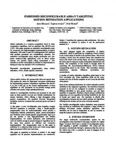
I. I NTRODUCTION Fast runtime partial reconfiguration features of embedded systems [9], [11] are available for programming the concept of dynamically reconfigurable computing by on-the-fly reorganizing of available cells in regular array structures such as those in FPGAs (Field-Programmable Gate Arrays). This is not only relevant to the composition of new embedded systems using architectures and procedural models that stem from the “designed for change” methodology but also can be of decisive importance during the perpetual process of upgrading existing evolution-capable embedded systems. Runtime reconfigurable computing supports many powerful features, including the following. If a new function cannot be immediately allocated due to lack of contiguous free cells, a suitable rearrangement of a subset of the functions currently running can solve the problem [4], [6], [16], [17]. A mechanism to fulfill such rearrangements without disturbing the system operation is illustrated in Fig. 1, where Fig. 1(b) shows the current configurations of two running functions, an incoming function is shown in Fig. 1(a) and the final configurations after runtime partial reconfiguration are depicted in Fig. 1(c). The continuity of this reorganization mechanism guarantees that invariants of the design are respected, dependencies can be detected, and the impact of planned changes can be determined. This paper is organized as follows. Section III discusses related work. Section IV presents some basic definitions. Section V covers the operators used in runtime reconfiguration. A set of rules for reconfiguration is presented in section VI and its reconfiguration consequence is given as an invariant
(a) An incoming function x
a
b
c
y
d
e
f
z
g
h
i
t
u
(b) The current configurations of two running functions a
b
c
1
2
d
e
f
3
4
g
h
i
5
6
x
y
z
t
u
(c) The final configurations after runtime partial reconfiguration Fig. 1.
Runtime partial reconfiguration
2
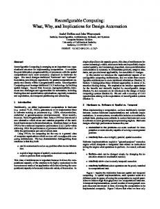
in section VII. Some algorithms for the reconfiguration are developed in sections VIII and IX. Finally, a short conclusion is given in section X. II. M OTIVATION For a diagram of runtime reconfigurable computing in a regular array structure such as in an FPGA, see Fig. 2. Any online management strategy implies a dynamic relocation mechanism of the available logic resources (L in the diagram), whereby the system tries to avoid a lack of contiguous free L resources from preventing the configuration of new functions (provided that the total number of L resources available is sufficient). If a new function cannot be allocated immediately due to lack of contiguous free L resources, a suitable rearrangement of a subset of the functions currently running can help to solve the problem. Any reconfiguration action must therefore ensure that the links from the original L are not broken before being totally re-established from its replica; otherwise its operation will be disturbed or even halted. For guaranteeing this continuity of development, various invariants of the design under the transformations must be respected.
L
c
L
c
L
c
s
c
s
c
L
c
L
c
L
Wiring segment
One cell
Horizontal Routing Channel
Channel segment c
s
c
s
c
L
c
L
c
L
Vertical Routing Channel
Fig. 2.
A regular array structure model
In this paper we consider and formalize the invariant for transformations as illustrated in Fig. 1 (i.e., restructuring of the configuration using reconfiguration rules). III. R ELATED W ORK In [4], [7], some of the opportunities for improving embedded software engineering technologies for requirements engineering and architecture design are discussed. When considering the embedded software development process, it is necessary to understand the context in which it is applied. Many familiar products today contain embedded software (for example, mobile telephones, DVD players, cars, airplanes, and medical systems). The software in these products constitutes only one important part. Embedded software engineering and other processes such as mechanical engineering and electrical engineering are in fact sub-processes of systems engineering. Coordinating these sub-processes to develop quality products
is one of most challenging aspects of embedded system development. The increasing complexity of such systems makes it impossible to consider these disciplines in isolation. Component-based software design has received considerable attention in industry and academia since object-oriented software development approaches have become popular. Recent years have seen the emergence of formal and informal techniques and technologies for the specification and implementation of component-based software architectures. With the growing need for safety-critical embedded software, this trend has become even more important. Formal methods [2], [10] have sometimes not kept up with the increasing complexity of software. For instance, a range of new middleware platforms have been developed in both enterprise and embedded systems industries. Engineers often use semi-formal notations such as UML to model and organize components into architectures. FESCA [14] addresses the open question of how formal methods can be applied effectively to these new contexts. In [8], a model-based design and analysis of componentbased embedded real-time software is described. All aspects of an embedded real-time system are captured in domain-specific models, including software components and architecture, timing and resource constraints, processes and threads, execution platforms, and so on. This can raise the level of abstraction for the designer and facilitate rapid system prototyping. In [13], a methodology of transforming structural models to runtime models with real-time constraints is considered. That method makes use of results from real-time scheduling theory and tries to obtain a runtime model that not only satisfies timing constraints but also yields high processor utilization and low overheads. The proposed approach is based on identifying transactions and assigning priorities to fine-granularity actions using the simulated annealing technique. As opposed to the traditional object-based or transaction-based approach, the approach in [13] yields higher processor utilization, lower implementation overheads and timing constraint satisfaction. It is possible to use diagrams as part of a formal mathematical proof [12]. More specifically for software, in [1], modelbased approaches to software development require languages and tools to support the creation and analysis, consistency management, refinement and implementation of models. In order to provide such support in a variety of contexts, efficient ways of designing languages have to be found, accepting that languages are evolving and that tools need to be delivered in a timely fashion. Thus, an engineering approach is required that allows for the generation of such tools from high-level specifications. Graph transformation provides such a high-level approach to diagrammatic languages, whose abstract syntax is naturally represented as a graph. Combined with techniques like meta modeling, compiler technology, logic and algebraic semantics, this provides a technological and semantic basis for the engineering of visual modeling languages. For reasoning about reconfiguration, we make use of the index-mapping concept presented in [5] and manipulate it to arrange the logical configuration formally, representing an application in a regular array structure with some forbidden cells due to occupation of some other applications or some
3
fault. The basic definitions in section IV are inspired by the index-mapping concept. Significantly, our rules of reconfiguration are be built from these concepts; the invariant is recognized under the restructure of configuration using the rules and our heuristic approach to dynamical reconfiguration is formally developed. By applying this heuristic, the problem of reconfiguring a running application dynamically is solved. IV. S OME BASIC D EFINITIONS Definition 4.1: Logical configuration A logical configuration is a set of logical index pairs (x, y) 6= (0, 0) of the abstract cells of regular array structure, namely working cells. In other words, a pair of logical indexes denotes the function performed by a working cell in the logical configuration. Any non-working cell, namely unused cell or spare, has its logical indexes set to (0, 0). The whole logical configuration is associated with an array L of logical indexes. Fig. 3 shows a regular array structure of 4 × 4 cells with two unused rows and two unused columns.
(0,0) (0,0) (0,0) (0,0) (0,0) (0,0) Fig. 3.
(0,0) (1,1) (2,1) (3,1) (4,1) (0,0)
(0,0) (1,2) (2,2) (3,2) (4,2) (0,0)
(0,0) (1,3) (2,3) (3,3) (4,3) (0,0)
(0,0) (1,4) (2,4) (3,4) (4,4) (0,0)
(0,0) (0,0) (0,0) (0,0) (0,0) (0,0)
A 4 × 4 array with the unused cells having (0, 0) logical indexes
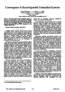
Definition 4.2: Reconfiguration Reconfiguration is as a transformation of the logical configuration by the reconfiguration rules. Note that, hereby, the meaning of reconfiguration and configuration transformation are similar and they are exchangeable in use. Definition 4.3: Locality Locality in reconfiguration is the predetermined bounds allowing each pair of logical indexes to be only transformed onto a restricted set of cells at limited distance from the current nominal position. The locality in reconfiguration is expressed by the adjacency domain notion. Definition 4.4: Adjacency domain An adjacency domain of cell (i, j) consists of precisely all cells onto which the logical index (i, j) can be transformed as a consequence of reconfiguration. Note that there are several available structures of adjacency domain based on this definition so we can choose one kind for reconfiguration. The number of rows and columns related to the directions and structure of the adjacency domains are illustrated in Fig. 4. For example, if the adjacency domain is defined as in Fig. 4(m), its cells will be on two columns and two rows. Formally, the adjacency domains are denoted by {(i, j), (i, j + 1)} for the diagram in Fig. 4(a), {(i, j), (i, j − 1)} for the diagram in Fig. 4(b),
{(i, j), (i − 1, j)} for the diagram in Fig. 4(c), {(i, j), (i + 1, j)} for the diagram in Fig. 4(d), {(i, j), (i − 1, j), (i, j − 1), (i, j + 1)} for the diagram in Fig. 4(e), {(i, j), (i, j − 1), (i, j + 1), (i + 1, j)} for the diagram in Fig. 4(f), {(i, j), (i − 1, j), (i, j + 1), (i + 1, j)} for the diagram in Fig. 4(g), {(i, j), (i − 1, j), (i, j − 1), (i + 1, j)} for the diagram in Fig. 4(h), {(i, j), (i, j + 1), (i + 1, j)} for the diagram in Fig. 4(i), {(i, j), (i − 1, j), (i, j + 1)} for the diagram in Fig. 4(j), {(i, j), (i − 1, j), (i, j − 1)} for the diagram in Fig. 4(k), {(i, j), (i, j − 1), (i + 1, j)} for the diagram in Fig. 4(l), {(i, j), (i − 1, j), (i, j − 1), (i, j + 1), (i + 1, j)} for the diagram in Fig. 4(m) Definition 4.5: Forbidden cell The cells of a regular array structure are occupied by some current logical configurations, namely forbidden cells. Alterternatively, there are forbidden-free cells, which can be allocated to a new logical configuration. Definition 4.6: Partially correct logical array Intermediate steps of a reconfiguration transformation lead to a partially correct logical array. This is defined as one in which: every logical index (i, j) appears once and only once; the adjacency domain structure is satisfied. Definition 4.7: Totally correct logical array The final reconfiguration results in a totally correct logical array, defined as one that, besides being partially correct, is also characterized as follows: all non-working cells are associated with the set of logical indexes to (0, 0); all nonzero logical indexes are associated with forbidden-free cells. V. RUNTIME R ECONFIGURATION O PERATORS From the definition of the adjacency domain, it can be seen that reconfiguration consists of a deformation of the nominal distribution of logical indexes onto the forbidden-free cells of a regular array structure and actually reconfiguration transformations are only the steps creating deformation lines. A deformation, which is a function of the given forbidden pattern, results in a deformation line. In other words, a deformation line is an abstract association that creates a correspondence between a forbidden cell and a forbidden-free unused cell. A deformation line consists of one vertical and one horizontal segment. A vertical deformation array, V , and a horizontal deformation array H represent these segments. Each entry of V and H can be either 0 or 1. Some vertical and horizontal deformation operators are associated with these arrays according to the chosen adjacency domain structure, see Fig. 4. In particular, the following operations will correspond to the adjacency domains. If the adjacency domain of (i, j) is {(i, j), (i, j +1)} then it needs only an eastward horizontal operator, OhE , which acts upon cell (i, j) and its adjacency in eastward. This will be denoted by {{(i, j), (i, j + 1)} : OhE }. Similarly, we also have the operators as follows: {{(i, j), (i, j − 1)} : OhW },
4
(i,j)
(i,j+1)
(i,j-1)
(a)
(i,j)
(b)
(i-1,j)
(i-1,j)
(i,j)
(i-1,j)
(i,j)
(i+1,j)
(c)
(d)
(i,j-1)
(i,j)
(i,j-1)
(i,j+1)
(i,j)
(i,j+1)
(i+1,j)
(e)
(f)
(i-1,j)
(i,j)
(i,j+1)
(i,j-1)
(i+1,j)
(g)
(i,j)
(i,j)
(i+1,j)
(i+1,j)
(h)
(i,j+1)
(i-1,j)
(i-1,j)
(i,j)
(i)
(i,j+1)
(j)
(i,j-1)
(i,j-1)
(i,j)
(i,j)
(k)
(i+1,j)
(l)
(i-1,j)
(i,j-1)
(i,j)
(i,j+1)
(i+1,j)
(m) Fig. 4.
The available adjacency domains of cell (i, j)
{{(i, j), (i − 1, j)} : OvN }, {{(i, j), (i + 1, j)} : OvS }, {{(i, j), (i − 1, j), (i, j − 1), (i, j + 1)} : OhE , OhW and OvN }, {{(i, j), (i, j − 1), (i, j + 1), (i + 1, j)} : OhE , OhW and OvS }, {{(i, j), (i − 1, j), (i, j + 1), (i + 1, j)} : OvN , OvS and OhE }, {{(i, j), (i − 1, j), (i, j − 1), (i + 1, j)} : OvN , OvS and OhW }, {{(i, j), (i, j + 1), (i + 1, j)} : OvS and OhE }, {{(i, j), (i − 1, j), (i, j + 1)} : OvN and OhE }, {{(i, j), (i − 1, j), (i, j − 1)} : OvN and OhW }, {{(i, j), (i, j − 1), (i + 1, j)} : OvS and OhW }, {{(i, j), (i − 1, j), (i, j − 1), (i, j + 1), (i + 1, j)} : OvN , OvS , OhE and OhW }. Note that when considering how operators O act and the nature of deformation arrays H and V , an important issue is the choice of the adjacency domain structure for use in the reconfiguration. As in Fig. 4, we can choose any of thirteen adjacency domain structures (from Fig. 4(a) to Fig. 4(m)) to reason about reconfiguration. We will consider the most complicated adjacency domain structure in Fig. 4(m) consisting of five cells {(i, j), (i, j − 1), (i, j + 1), (i − 1, j), (i + 1, j)}; reasoning about other structures is much the same. We say that Oh = OhE or OhW , Ov = OvN or OvS . Operator Oh , which acts upon the logical array L using horizontal deformation array H, creates a horizontal deformation segment, M (i, j) = Oh (H(i, j), L(i, j)). Similarly, operator Ov , which acts upon the logical array L using vertical deformation
array V , creates a vertical deformation segment, N (i, j) = Ov (V (i, j), L(i, j)) and a combination of horizontal and vertical deformation segments will create a deformation line of logical index, P (i, j) = Ov (V (i, j), Oh (H(i, j), L(i, j))). Let the deformation line connect a forbidden cell (i, j) with an unused cell (is , js ); two arrays H and V can be created according to location of (is , js ) as follows: If (is , js ) is in the right column then • i ≤ is H(is , r) = 1, j + 1 ≤ r ≤ js V (t, j) = 1, i + 1 ≤ t ≤ is • i > is H(is , r) = 1, j + 1 ≤ r ≤ js V (t, j) = 1, is ≤ t ≤ i − 1 If (is , js ) is in the left column then • i ≤ is H(is , r) = 1, js ≤ r ≤ j − 1 V (t, j) = 1, i + 1 ≤ t ≤ is • i > is H(is , r) = 1, js ≤ r ≤ j − 1 V (t, j) = 1, is ≤ t ≤ i − 1 If (is , js ) is in the top row then • j ≤ js
5
P P P P P P Fig. 5.
P C F C C P
P C C C C P
P C C C C P
P P P P P P
0 0 0 0 0 0
The situation of configuration cells
(0,0) (0,0) (0,0) (0,0) (0,0) (0,0) Fig. 6.
P C C C C P
(0,0) (1,1) (2,1) (3,1) (4,1) (0,0)
(0,0) (1,2) (2,2) (3,2) (4,2) (0,0)
(0,0) (1,3) (2,3) (3,3) (4,3) (0,0)
Fig. 7.
(0,0) (1,4) (2,4) (3,4) (4,4) (0,0)
0 0 0 0 0 0
Forbidden cell (2, 2) associated with unused (4, 5) cell
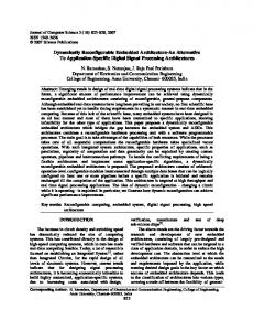
If (is , js ) is in the lower row then • j ≤ js H(is , r) = 1, j + 1 ≤ r ≤ js V (t, j) = 1, i + 1 ≤ t ≤ is • j > js H(is , r) = 1, js ≤ r ≤ j − 1 V (t, j) = 1, i + 1 ≤ t ≤ is Example: Consider the example shown in Fig. 5 to 10, where the symbols C, F, P in Fig. 5 denote, respectively, the correctly working, forbidden, and unused cells. Assume a forbidden cell (2, 2) has been associated with unused (4, 5). Fig. 6 to 10 indicate the initial logical array, the horizontal deformation array H, and the vertical deformation array V . Note that, given the constraints posed by the adjacency domain structure and the operations Oh and Ov , two unused columns and two unused rows can be added to the array for subsequent reconfiguration actions. We apply the operations O above to create H and V for each forbidden cell. More than one deformation line is present, each connecting a forbidden cell with an unused cell. By some consistent changes in processing, we develop runtime operators. Operator OhE [or OhW ] OhE [OhW ] acts upon the logical array L using horizontal deformation array H with the east-to-westward (or west-toeastward) order of deformation action to create a horizontal deformation segment, the duplication of cell and connections to them before doing the next deformation action. The
Fig. 8.
0 0 0 0 0 0
0 0 0 0 1 0
0 0 0 0 1 0
0 0 0 0 1 0
Array H for the forbidden cell (2, 2) and unused (4, 5) cell
(0,0) (0,0) (0,0) (0,0) (0,0) (0,0)
H(is , r) = 1, j + 1 ≤ r ≤ js V (t, j) = 1, is ≤ t ≤ i − 1 • j > js H(is , r) = 1, js ≤ r ≤ j − 1 V (t, j) = 1, is ≤ t ≤ i − 1
0 0 0 0 0 0
0 0 0 0 0 0
0 0 0 1 1 0
0 0 0 0 0 0
0 0 0 0 0 0
0 0 0 0 0 0
Array V for the forbidden cell (2, 2) and unused (4, 5) cell
intermediate logical array M = OhE (H, L) [OhW (H, L)] is determined by the following operations. (i)For k = js downto [to] j + 1 [j − 1] do begin H(is , k) = 1 ⇐⇒ M (is , k) = L(is , k − 1) [L(is , k + 1)]; Determine the set of connections of the cell corresponding to L(is , k − 1) [L(is , k + 1)]; i.e., C(L(is , k − 1)) [C(L(is , k + 1))]; Determine the set of connections of the cell corresponding to M (is , k); i.e., C(M (is , k)). In fact, it is easy to see C(M (is , k)) = Ø; Add the connections to cell corresponding to M (is , k) that
(0,0) (0,0) (0,0) (0,0) (0,0) (0,0) Fig. 9.
(0,0) (1,2) (2,2) (3,2) (0,0) (0,0)
(0,0) (1,3) (2,3) (3,3) (4,2) (0,0)
(0,0) (1,4) (2,4) (3,4) (4,3) (0,0)
(0,0) (0,0) (0,0) (0,0) (4,4) (0,0)
E to skip the cell (2, 2) using unused (4, 5) cell Running the Oh
(0,0) (0,0) (0,0) (0,0) (0,0) (0,0) Fig. 10.
(0,0) (1,1) (2,1) (3,1) (4,1) (0,0)
(0,0) (1,1) (2,1) (3,1) (4,1) (0,0)
(0,0) (1,2) (0,0) (2,2) (3,2) (0,0)
(0,0) (1,3) (2,3) (3,3) (4,2) (0,0)
(0,0) (1,4) (2,4) (3,4) (4,3) (0,0)
(0,0) (0,0) (0,0) (0,0) (4,4) (0,0)
Running the OvS to skip the cell (2, 2) using unused (4, 5) cell
6
0 0 0 0 0 0
0 0 0 0 0 0
0 0 0 0 0 0
0 0 0 0 1 0
0 0 0 0 1 0
0 0 0 0 1 0
(4 ,1 ) (4 ,2) (4 ,3 ) (4 ,4 ) (4 ,4 )
(4 ,1 ) (4 ,2) (4 ,3 ) (4 ,4 ) (0 ,0 )
(a) The array H
(b) A portion of logical index row 4 processed
(c)
(4 ,1 ) (4 ,2) (4 ,2 ) (4 ,3 ) (4 ,4 )
(4 ,1 ) (0 ,0 ) (4 ,2) (4 ,3 ) (4 ,4 )
(4 ,1 ) (4 ,2) (4 ,3 ) (4 ,3 ) (4 ,4 ) H(is,k)=1 ⇔ M (is,k) = L (is,k-1) i.e., H(4,4)=1 ⇔ M (4,4) = L (4,3)
H(is,k)=1 ⇔ M (is,k) = L (is,k-1) i.e., H(4,3)=1 ⇔ M (4,3) = L (4,2)
(d)
H(is,k)=0 and H(is,k+1)=1 ⇔ M (is,k) = (0,0) i.e., H(4,1)=0 and H(4,2)=1 ⇔ M (4,1) = (0,0)
(e)
0 0 0 0 0 0
0 0 0 0 0 0
0 0 0 1 1 0
0 0 0 0 0 0
0 0 0 0 0 0
(g) The array V
(2 ,2 ) (2 ,2 )
0 0 0 0 0 0
(f)
(2 , 2 )
(2 ,2 )
(3 ,2 )
(3 ,2 )
(0 , 0 )
(3 ,2 )
V(k,js)=1 ⇔ N (k,js) = L (k-1,js) i.e., V(4,2)=1 ⇔ N (4,2) = L (3,2)
(h) A portion of logical index column 2 processed
V(k,js)=1 ⇔ N (k,js) = L (k-1,js) i.e., V(3,2)=1 ⇔ N (3,2) = L (2,2)
(3 ,2 )
(i)
(0 ,0 ) (2 ,2 )
V(k,js)=0 and V(k+1,js)=1 ⇔ N (k,js) = (0,0) i.e., V(2,2)=0 and V(3,2)=1 ⇔ N (2,2) = (0,0)
(3 ,2 ) (j)
Fig. 11.
H(is,k)=1 ⇔ M (is,k) = L (is,k-1) i.e., H(4,5)=1 ⇔ M (4,5) = L (4,4)
(k)
E and O S to skip the forbidden cell (2, 2) using unused (4, 5) Running the runtime Oh v
are same as ones corresponding to L(is , kS− 1) [L(is , k + 1)]; i.e., C(M (is , k)) = C(M (is , k)) C(L(is , k − 1)) [C(L(is , k + 1))] = C(L(is , k − 1)) [C(L(is , k + 1))]; Release the connections to cell corresponding to L(is , k − 1)[L(is , k + 1)]; i.e., C(L(is , k − 1)) = C(L(is , k − 1))\C(L(is , k − 1)) [C(L(is , k + 1)) = C(L(is , k + 1))\C(L(is , k + 1))] = Ø; end H(is , j) = 0 and H(is , j + 1) [H(is , j − 1)] = 1 ⇐⇒ M (is , j) = (0, 0); (ii) H(i, j) = 0 and H(i, j + 1) [H(i, j − 1)] = 0 ⇐⇒ M (i, j) = L(i, j) Operator OvS [or OvN ] OvS [OvN ] acts upon the logical array L using vertical
deformation array V with the south-to-northward (or northto-southward) order of deformation action to create a vertical deformation segment, the duplication of cell and connections to them before doing the next deformation action. The intermediate logical array N = OvS (V, L) [OvN (V, L)] is determined by the following operations: (i) For k = is downto [to] i + 1 [i − 1] do begin V (k, js ) = 1 ⇐⇒ N (k, js ) = L(k − 1, js ) [L(k + 1, js )]; Determine the set of connections of the cell corresponding to L(k − 1, js ) [L(k + 1, js )]; i.e., C(L(k − 1, js )) [C(L(k + 1, js ))]; Determine the set of connections of the cell corresponding to N (k, js ); i.e., C(N (k, js )). In fact, it is easy to see C(N (k, js )) = Ø;
7
Add the connections to cell corresponding to N (k, js ) that are same as ones corresponding to L(k −S 1, js ) [L(k + 1, js )]; i.e., C(N (k, js )) = C(N (k, js )) C(L(k − 1, js )) [C(L(k + 1, js ))] = C(L(k − 1, js )) [C(L(k + 1, js ))]; Release the connections to cell corresponding to L(k − 1, js ) [L(k+1, js )]; i.e., C(L(k−1, js )) = C(L(k−1, js ))\C(L(k− 1, js )) [C(L(k + 1, js )) = C(L(k + 1, js ))\C(L(k + 1, js ))] = Ø; end V (i, js ) = 0 and V (i + 1, js ) [V (i − 1, js )] = 1 ⇐⇒ N (i, js ) = (0, 0); (ii) V (i, j) = 0 and V (i + 1, j) [V (i − 1, j)] = 0 ⇐⇒ N (i, j) = L(i, j) Example: As in Fig. 5 to 10, the tables in Fig. 11 illustrate in detail the order of operations of OhE , OvS based on the arrays H and V . VI. R ECONFIGURATION RULES Until now, we have been able to formulate the reconfiguration rules as follows: All forbidden-free cells Rule M.1.1. If the cell (i, j) is uninvolved then it is a corresponding target of logical index (i, j) There exists a forbidden cell Rule M.2.1. If the cell (i, j) is forbidden, an unused cell (is , js ) on the right column and i ≤ is then create the arrays H, V after that applying the operators OhE (H, L) and OvS (V, L). M.2.1 It will be denoted by h(i, j), (is , js ), i ≤ is , j < js i =⇒ E S hH, Oh (H, L)i and hV, Ov (V, L)i Rule M.2.2. M.2.2 h(i, j), (is , js ), i > is , j < js i =⇒ hH, OhE (H, L)i and N hV, Ov (V, L)i i.e., if the cell (i, j) is forbidden, an unused cell (is , js ) on the right column and i > is then create the arrays H, V after that applying the operators OhE (H, L) and OvN (V, L). Rule M.2.3. M.2.3 h(i, j), (is , js ), i ≤ is , j > js i =⇒ hH, OhW (H, L)i and S hV, Ov (V, L)i i.e., if the cell (i, j) is forbidden, an unused cell (is , js ) on the left column and i ≤ is then create the arrays H, V and applying the operators OhW (H, L) and OvS (V, L). Rule M.2.4. M.2.4 h(i, j), (is , js ), i > is , j > js i =⇒ hH, OhW (H, L)i and N hV, Ov (V, L)i i.e., if the cell (i, j) is forbidden, an unused cell (is , js ) on the left column and i > is then create the arrays H, V and applying the operators OhW (H, L) and OvN (V, L). Rule M.2.5. M.2.5 h(i, j), (is , js ), i < is , j ≤ js i =⇒ hV, OvN (V, L)i and E hH, Oh (H, L)i i.e., if the cell (i, j) is forbidden, an unused cell (is , js ) on
the top row and j ≤ js then create the arrays H, V and applying the operators OvN (V, L) and OhE (H, L). Rule M.2.6. M.2.6 h(i, j), (is , js ), i < is , j > js i =⇒ hV, OvN (V, L)i and hH, OhW (H, L)i i.e., if the cell (i, j) is forbidden, an unused cell (is , js ) on the top row and j > js then create the arrays H, V and applying the operators OvN (V, L) and OhW (H, L). Rule M.2.7. M.2.6 h(i, j), (is , js ), i > is , j ≤ js i =⇒ hV, OvS (V, L)i and hH, OhE (H, L)i i.e., if the cell (i, j) is forbidden, an unused cell (is , js ) on the lower row and j ≤ js then create the arrays H, V and applying the operators OvS (V, L) and OhE (H, L). Rule M.2.8. M.2.8 h(i, j), (is , js ), i > is , j > js i =⇒ hV, OvS (V, L)i and hH, OhW (H, L)i i.e., if the cell (i, j) is forbidden, an unused cell (is , js ) on the lower row and j > js then create the arrays H, V and applying the operators OvS (V, L) and OhW (H, L). VII. R ECONFIGURATION C ONSEQUENCE AS AN I NVARIANT We will show that the reconfiguration consequence is just an invariant in this section. 1) Reconfiguration consequence: A logical array X is a reconfiguration consequence of L (written L |⊂ X) iff the partial correction of L is also preserved in X. 2) Provability: A logical array X is provable from L (written L ` X) iff X is a result of L by the reconfiguration rules. Before considering the soundness of the reconfiguration rules we prove the following lemmas. Lemma 7.1: Rule M.1.1 creates a partially correct logical array Proof: This follows from the definition 4.6 Lemma 7.2: Rule M.2.1 creates a partially correct logical array Proof: A partial correction must satisfy two constraints that every logical index L(i, j) 6= (0, 0) is not duplicated and that the logical index L(i, j) = (0, 0) does not appear in X due to the locality of the cell adjacency domain (as in the definition of partially correct logical array above). We will prove that any logical array created by rule M.2.1 satisfy these above two constraints. Firstly, we prove every logical index L(i, j) 6= (0, 0) is not duplicated by rule M.2.1. Let the logical indexes X(i0 , j 0 ) and X(i”, j”) be not (0, 0) and L be a partially correct logical array. Suppose that (i, j) be a cell with initial logical indexes L(i, j) = X(i0 , j 0 ) = X(i”, j”). This cell is unique from the definition of L as a partially correct logical array. For the eastward horizontal operator OhE (H, L) of rule M.2.1, it is i = i0 = i”. By operation (i) of OhE (H, L), j 0 = j” = j − 1 or by operation (ii) of OhE (H, L), j 0 = j” = j, if j 0 6= j” then j 0 = j and j” = j + 1 or vice versa. By operation (i), if j” = j +1 = j 0 +1 then H(i0 , j 0 +1) = 1. By operation (ii), if j 0 = j then H(i0 , j 0 ) = 0. By operation (i), if H(i0 , j 0 +1) = 1
8
and H(i0 , j 0 ) = 0 then X(i0 , j 0 ) = (0, 0). This contradicts the hypothesis of logical indexes X(i0 , j 0 ) 6= (0, 0). Hence, every logical index L(i, j) 6= (0, 0) is not duplicated under the operator OhE (H, L). In the same way, every logical index L(i, j) 6= (0, 0) is not also duplicated under the southward vertical operator OvS (V, L). Secondly, we prove that the logical indexes L(k, h) = (0, 0) do not appear in X. Suppose that L is a partially correct logical array and L(i, j) 6= (0, 0) for each cell for which H(i, j) = 1 and H(i, j + 1) = 0. Due to H(i, j) = 1, then X(i, j) = L(i, j −1) by operation (i) of OhE (H, L). X(i, j +1) = L(i, j) iff H(i, j+1) = 1 by operation (i) as well. This contradicts the above hypothesis; hence the logical indexes that do not appear in X are zero in L under the operator OhE (H, L). Similarly, under the operator OvS (V, L), the logical indexes L(k, h) = (0, 0) do not also appear in X; see an illustration in Fig. 12. X, created from L by rule M.2.1, is then partially correct. H (i,j)=1 H (i,j+1)=0
H (i,j+2)=1
x1 x2 xi+1 xi+2 … … xki+1 xki+2
xi … … x2i … … … x(k+1)i
(a)
y1 yj+1 y2j+1 … ypj+1
y2 yj+2 y2j+2 … ypj+2
y3 yj+3 y2j+3 … ypj+3
yj … … y2j … y3j … … … y(p+1)j
(b)
x1 x2 ... x(k+1)i
y1 x x … x
y2 x x … x
y3 x x … x
… … … … …
y(p+1)j x x … x
(c) Fig. 13. Labels of logical indexes (in 13(a)), cells (in 13(b)) and the coverage table (in 13(c)).
�
(i,j)≠(0,0) H�(i,j)=1
�
(i,j)=
(i,j-1)
�
�
(i,j+1)=(0,0)
H�(i,j+1)=1
�
(i,j+1)=
(i,j)
�
Fig. 12. Logical index L(i, j + 1) = (0, 0) does not appear in X under the E (H, L) operator Oh
Lemma 7.3: Every rule of M.2.2, M.2.3, M.2.4, M.2.5, M.2.6, M.2.7 and M.2.8 creates a partially correct logical array Proof: The proof steps are similar to those for lemma 7.2. Theorem 7.4 (Soundness): If L ` X then L |⊂ X Proof: This is a consequence of the lemmas 7.1, 7.2, and 7.3 above. VIII. R ECONFIGURATION AS A C OMPLETE M ATCHING P ROBLEM Reconfiguration is now defined simply as the search for a mapping of logical indexes onto configuration cells, given a predetermined adjacency domain of cells. It will be seen that such a problem can be described by means of a complete matching problem [3]. Let X = {x1 , x2 , . . . , xm } and Y = {y1 , y2 , . . . , yn } be two finite sets with m logical indexesTand n forbidden-free cells, respectively. It is obvious that X Y = Ø. Let 4 be a collection of pairs e = {x, y} where x ∈ X and y ∈ Y . The triple GS = (X, 4, Y ) is called a bipartite graph. The elements of X Y are called the vertices of G, and X,Y is called a bipartition (partition into two parts) of the vertices of G. The pairs e = {x, y} in 4 are called the edges of G,
each edge e = {x, y} is a set of two vertices, one of which, x, comes from X and the other of which, y, comes from Y . We say that the edge e joins the vertices x and y, and that the vertices x and y meet the edge e. Thus a bipartite graph is represented by: (i) A set of vertices; (ii) A partition of that set of vertices into two parts of X and Y ; and (iii) A set 4 of edges joining a vertex in one part X to a vertex in the other part Y , and |4| = m × n. Reconsidering Fig. 5 to 10, we can draw the coverage table representing the relation between the logical indexes in rows and the forbidden-free cells in columns. This table can be considered as the incidence matrix of a bipartite graph, where: (i) Rows (i.e., logical indexes) correspond to the set of X; (ii) Columns (i.e., forbidden-free cells) correspond to the set of Y ; (iii) There is an edge (xi , yj ) from a vertex of xi ∈ X to a vertex of yj ∈ Y iff there is a mark in row xi , column yj of the coverage table. In this case, for simplifying the representation, we label the rows corresponding to logical indexes and columns corresponding to cells as in Fig. 13. We associate with Fig. 13(c) a bipartite graph as follows. Corresponding to each row of the table there is a left vertex: xi , i = 1, 2, . . . , (k + 1)i. Corresponding to each column of the table there is a right vertex: yj , j = 1, 2, . . . , (p + 1)j of the forbidden-free cells. Note that all forbidden cells will not be labeled and will also not be in table. The sets of left and right vertices are, respectively, X = {xi : i = 1, 2, . . . , (k + 1)i} and Y = {yj : j = 1, 2, . . . , (p + 1)j}. In G we join vertex xi and vertex yj by an edge iff the intersection of row i and column j is marked. We let 4 be the set of edges obtained in this way and then define a bipartite graph G by G = (X, 4, Y ). The
9
set 4 of edges of G is in 1-1 correspondence with the marks of the table. IX. A H EURISTIC FOR R ECONFIGURATION Prior to describing the algorithmic approach using our heuristic for matching, some definitions are presented. Definition 9.1: Matching A match M is a subset of edges of G(M ⊂ 4) such that no two edges have an end-point in common. Definition 9.2: Maximum matching A match is called maximum if no other match contains more edges. To solve the reconfiguration problem, our heuristic is specified with respect to three issues for problem solving [15]: representation of search space, objective and starting point. A. Representation of search space We will encode alternative candidate solutions for manipulation. In other words, the representation of a potential match and its corresponding interpretation implies the search space and its size. For this purpose, the coverage table is considered as a representation of search space of potential matches. Let S be the search space of potential maximum matches. Each element x of S is a maximum match and must satisfy the following two conditions: (i) Each logical index must be associated with a cell, so there is one mark in each row of coverage table. (ii) No cell can be associated with more than one logical index, so there is at most one mark in each column. The size of S is the number of different maximum matches in S, written as |S|, and determined as follows. Let n and m be the number of columns and rows of coverage table respectively, where n ≥ m. It is obvious that the value of |S| is just the largest number of maximum matches. In other words, it is calculated by the following expression: |S| = n × (n − 1) × (n − 2) × . . . × (n − m), where n is the number of possible selections of a mark on the first row, (n − 1) corresponds to the number of possible selections of a mark on the second row, . . ., and (n − m) corresponds to the number of possible selections of a mark on the mth row. B. Objective Once we defined the search space, we have to decide for what it is that we are searching. What is the objective of our problem? This should be a mathematical statement of the task to be achieved. Here, the objective is typically any maximum match that satisfies the total correction of a logical array. In mathematical terms, let Ssol be a set of the solutions (i.e., the maximum matches satisfying the total correction of the logical array). Hence, Ssol ⊂ S and our objective is to find any maximum match x ∈ Ssol ⊂ S. To build Ssol we separate it into two cases, existing forbidden-free and forbidden cells. If all forbidden-free cells then Ssol = {(xi , yi ), i = 1, 2, . . . , m} as a result of applying rule M.1.1 and in this case x is easy to determine: x = {(xi , yi ), i = 1, 2, . . . , m} ∈ Ssol . If there are some forbidden
cells then we realize that each cell in distribution of forbidden cells has potential correspondence with unused cells for the reconfiguration as described in the coverage table in Fig. 14, where F = {fi : i = 1, 2, . . . , k} is set of the forbidden cells and P = {pj : j = 1, 2, . . . , k} is set of the unused cells. This coverage table is considered as a representation of the solution space Ssol of potential reconfigurations, in which each element x of Ssol is a maximum match and must satisfy two following conditions: (i) Each forbidden cell must be associated with an unused cell, so there is one mark in each row of coverage table. (ii) No unused cell can be associated with more than one forbidden cell, so there is at most one mark in each column. Each component of element x ∈ Ssol (i.e., each selected mark in the coverage table in Fig. 14) related to reconfiguring the corresponding location of cells between a forbidden cell and unused cell is defined by one of the following rules: M.2.1, M.2.2, M.2.3, M.2.4, M.2.5, M.2.6, M.2.7 or M.2.8. The size of Ssol is the largest number of different maximum matches in Ssol , written as |Ssol |. This is determined by the following expression: |Ssol | = k × (k − 1) × (k − 2) × . . . × 2 × 1, where k is the number of possible selections of a mark on the first row, (k − 1) is the number of possible selection of a mark on the second row, . . ., and in the last case, there is one possible selection of a mark on the k th row.
x1 x2 ... x(k+1)i Fig. 14.
y1 x x … x
y2 x x … x
y3 x x … x
… … … … …
y(p+1)j x x … x
Coverage table of solution space Ssol .
C. Starting point So far we built up our solution space Ssol ⊂ S. A question to consider is which x ∈ S should be selected as starting point to arrive at a solution y ∈ Ssol ? In this case, we always choose the starting point x = {(xi , yi ) : i = 1, 2, . . . , m} ∈ S as a one-to-one relation between logical indexes and cells. Therefore, if there are only forbidden-free cells, x is a single solution (rule M.1.1); otherwise from starting point x we apply one of rules M.2.1–M.2.8 to each forbidden cell fi (i = 1, . . . , k) corresponding to a selected unused cell pj (j = 1, . . . , k); by the end, we will definitely reach a solution y ∈ Ssol . D. Sequential reconfiguration algorithm The following is a structure of our reconfiguration algorithm based on the heuristic approach presented above. Suppose that |P | ≥ |F |. Procedure Sequential-Reconfiguration; begin initialize a starting point x = {(xi , yi ) : i = 1, 2, . . . , m} ∈ S;
10
if F = Ø then run the rule M.1.1; while F 6= Ø do begin select f ∈ F ; select p ∈ P ; run one of rules M.2.1-M.2.8 according to the relation of location between f and p; F = F \{f }; P = P \{p}; end end Analysis and computational complexity of sequential reconfiguration algorithm: The computational complexity implies the computational time, which is just the time needed for computing the deformation operations in the selected rules M.2.1–M.2.8 in all iterations of the while loop. In other words, the computational time measured by the number of values 1 in the arrays H and V of the deformation operations because each value 1 in the arrays H and V determines a horizontal and vertical move respectively. Let 1(H) and 1(V ) be the functions determining the number P of values 1 in the array H and V ; then hij , P they are 1(H) = with ∀hij ∈ H and 1(V ) = vij , with ∀vij ∈ V . In each iteration of the while loop, the number ofPhorizontal P and vertical moves are 1(H) + 1(V ) = hij + vij , with ∀hij ∈ H and ∀vP ij ∈ V , and the total number of moves for all iterations are |F | (1(H) + 1(V )), where |F | is equal to the number of elements of the set F . Therefore its complexity is O(|F |n), where n = max(1(H) + 1(V )) over the set F . In determining this computational complexity, we realize that to reduce the number of moves 1(H) + 1(V ), we must suitably select the pair of (f, p) so that ∀f, ∃p: minimal (1(H) + 1(V )); i.e., local minimum (1(H) + 1(V )) or min(1(H) + 1(V P )) for short and the total number of moves of all iterations are |F | min(1(H) + 1(V )). This is just the reduced number of computations of the following Reconfiguration* algorithm, modified from the earlier Reconfiguration algorithm. Procedure Sequential-Reconfiguration*; begin initialize a starting point x = {(xi , yi ) : i = 1, 2, . . . , m} ∈ S; if F = Ø then run the rule M.1.1; while F 6= Ø do begin select f ∈ F ; select p ∈ P so that ∀f, ∃p: min(1(H) + 1(V )); run one of rules M.2.1-M.2.8 according to the relation of location between f and p; F = F \{f }; P = P \{p}; end end Illustration: We can manipulate the reconfiguration algorithm
to arrange a logical configuration into the variform portions of a regular array structure, provided that the number of cells required in each portion is available.
P1 C C C P4
P2 C C C P5
P3 C C C P6
F1 F3 F5
F2 F4 F6
(a)
(1,1) (2,1) (3,1)
(1,2) (2,2) (3,2)
(1,3) (2,3) (3,3)
(1,4) (2,4) (3,4)
(1,5) (2,5) (3,5)
(b)
(1,1) (2,1) (3,1) (2,4) (2,2)
(1,2) (1,3) (2,3) (3,4) (3,2)
(1,4) (1,5) (2,5) (3,5) (3,3)
(c) Fig. 15. Arranging a logical configuration in Fig. 15(b) into a portion in Fig. 15(a), and a solution in Fig. 15(c).
Given a portion size 5 × 3, in which we want to arrange a logical configuration size 3 × 5. As in Fig. 15(a), the portion labeled C for working cells and P for unused cells; however let us imagine there are further six unreal forbidden cells, labeled F, only for the purpose of corresponding to the logical configuration in Fig. 15(b). The C and F cells in Fig. 15(a) correspond to the logical configuration in Fig. 15(b). A solution in its solution space can be reached using the reconfiguration algorithm in Fig. 15(c); its number of moves P are calculated as ( [1(H) + 1(V )] = 22), as shown in Fig. 16(a). Note that confusion is avoided since the violation on the adjacent domain structure when we use the same logical indexes of the original configuration to indicate the last configuration in Fig. 15(c). The adjacent domain structure is only between two consecutive steps of configuration change. As a further calculation, it is easy to reach the values of moving of all solutions in its solution space, as in Fig. 16(b). From these values, it is useful to evaluate a potential solution with its minimal computational complexity by the relations between number of moves, F cells and P cells; see Fig. 16(c) and 16(d) for conducting the process of the Reconfiguration* algorithm mentioned above and hence improving the performance of the dynamic reconfiguration system. E. Parallel reconfiguration algorithm We now present a kind of the shared memory multitasking programming approach to reconfiguration, where our reconfiguration is allowed to consist of multiple processes executing concurrently. The method uses data partitioning. We suppose that there is a set of available processors, CP U s, which are activated by the statement For all CP U s in Parallel do . . .
11
P1 F1 F2 F3 F4 F5 F6
P2 3
P3
P4
P5
P6
Calculation
3
1(H) + 1(V) =2+1 1(H) + 1(V) =1+1 1(H) + 1(V) =2+2 1(H) + 1(V) =1+2 1(H) + 1(V) =3+3 1(H) + 1(V) =3+1 Σ[1(H) + 1(V)] =22
2 4 6 4
(a)
F1 F2 F3 F4 F5 F6
P1 4 4 5 5 6 6
P2 3 3 4 4 5 5
P3 2 2 3 3 4 4
P4 6 6 5 5 4 4
P5 5 5 4 4 3 3
old parent process, with the same data, and access rights to shared memory. For synchronization, a barrier is a synchronization point used to make sure that all processes executing a barrier call arrive and wait at the synchronization point before proceeding. The statement m sync(n) means that there is a barrier call to synchronize the n child processes. For an illustration of forking and barrier synchronization, see Fig. 17.
P6 4 4 3 3 2 2
CPUs m_fork(n) CPU 1
Compute
(b)
...
CPU i
...
Compute
CPU n
Compute
Idle Idle
Computational Complexity
(Complexity,F Cells)=P Cells
m_sync(n)
Fig. 17.
8 6
P1
4
P2
Statements of m fork() and m sync().
P3
2
P4
0
Fig. 16. Number of moves (in 16(a)), of all solutions (in 16(b)) and computational complexity between F cells and P cells (in 16(c) and 16(d).
Procedure Parallel-Reconfiguration; begin initialize a starting point x = {(xi , yi ) : i = 1, 2, . . . , m} ∈ S; For all CP U s in Parallel do if F = Ø then CP U (run the rule M.1.1); while F 6= Ø do begin Tn ∀fi ∈ F, ∃pj ∈ P : i=1 (fi , pj ) = Ø; m fork(n); kni=1 CP Ui ((fi , pj )) using rules M.2.1-M.2.8; m sync(n); Tn Sn F = F \ Si=1 {fi : Ti=1 (fi , pj ) = Ø}; n n P = P \ i=1 {pj : i=1 (fi , pj ) = Ø}; end end For all end
end For all, allowing them to be ready to start processing. A process running under CP U ∈ CP U s, invoked by the statement CP U (. . .) and the process including the n parallel child processes on n processors CP Ui ∈ CP U s (i = 1, . . . , n) by the statement kni=1 CP Ui (. . .). For data partitioning, let the pair of (fi , pj ) denote the set of relevant logical indexes in its horizontal andTvertical deforman tion operations. So ∀fi ∈ F, ∃pj ∈ P : i=1 (fi , pj ) = Ø (n ≥ 1) means that there exists n horizontal and vertical deformation operations that are data-independent; i.e., they read and write the different data. For process creation, a new process is usually created using a system call named m fork(. . .). The statement m fork(n) means a process is divided into n child processes for running in parallel. Each new child process is a duplicate copy of the
Analysis and computational complexity of parallel reconfiguration algorithm: In each iteration of the while loop, the number of horizontal and vertical moves are determined by the longest process CP Ux (x = 1 or 2 or . . . or n) among n parallel processes P n kP hij + i=1 CP Ui ((fi , pj )) as follows: 1(Hx ) + 1(Vx ) = vij , with ∀hij ∈ Hx and ∀vij ∈ Vx (Hx and Vx are the H and V matrices of process P CP Ux ). The total number of moves for all iterations are ite (1(Hx ) + 1(Vx )), with ite indicating the number of iterations of while loop. From determining this computation, we realize that its worst case is exactly the computation of the related sequential solution andP its best case is just whenPite = 1 (i.e., 1(Hx ) + 1(Vx ) ≤ ite (1(Hx ) + 1(Vx )) ≤ |F | (1(H) + 1(V ))). Therefore its complexity will be between O(n) and O(|F |n) P (i.e., O(n) ≤ O( ite (1(Hx ) + 1(Vx ))) ≤ O(|F |n)).
P5 F1
F2
F3
F4
F5
F6
P6
Forbidden Cells
(c)
Computational Complexity
(Complexity,P Cells)=F Cells 8 6
F1
4
F2 F3
2
F4
0
F5 P1
P2
P3
P4
P5
P6
F6
Spare Cells
(d)
12
Illustration: Referring back to the illustration in Fig. 15(a) and 15(b) above, this time we consider processing by the parallel reconfiguration algorithm. We immediately realize that the connection between fi and pj can be partitioned into some pairs of (fi , p Tjn) to reach a solution under the constraint ∀fi ∈ F, ∃pjT∈ P. i=1T (fi , pj ) = Ø as follows: (f1 , p3 ) T (f3 , p2 ) T (f5 , p1 ) = Ø (f2 , p4 ) (f4 , p5 ) (f6 , p6 ) = Ø P and its number of moves are calculated as ( 2 [1(Hx ) + 1(Vx )] = 12), as shown in Fig. 18(a). As a comparison, if this solution isP reached by the sequential algorithm its computation will be ( [1(H) + 1(V )] = 24), as in Fig. 18(b). Obviously, this parallel approach improves the performance better than the sequential one with reduced computation time.
P1 F1 F2 F3 F4 F5 F6
P2
P3
P4
P5
P6
P5
P6
6
6 (a)
P1 F1 F2 F3 F4 F5 F6
P2
P3 2
P4 6
4 4 6 2 (b)
Fig. 18. Number of moves of parallel solution (in 18(a)) and serial solution (in 18(b)).
X. C ONCLUSION For the continuous evolution of dynamically reconfigurable computing in embedded systems, we have considered how to reconfigure an embedding of a graph into a regular array using graph transformations. These transformations are bounded by adjacency constraints, which mean that connected nodes of a graph are still embedded adjacently after the execution of a graph transformation rule. An important contribution is that using the suggested approach, continuous evolution of the applications can be partially carried out at runtime without stopping the operation of the whole system. The continuity of this reorganization mechanism guarantees that invariants of the design are respected, dependencies can be detected and the impact of planned changes can be determined. Dynamic reconfiguration is likely to become increasingly important in embedded systems to allow increased flexibility.
However, the added complexity can create additional opportunities for errors in such systems. Particularly in safetycritical or security-critical applications, it will be important to use formal techniques to avoid the introduction of errors. In such cases, it is hoped that a rigorous approach such as that presented in this paper will be applied. R EFERENCES [1] G. Allwein and J. Barwise, Logical Reasoning with Diagrams, Oxford, England: Oxford University Press, 1996. [2] J. P. Bowen and M. G. Hinchey, Formal methods, in A. B. Tucker, Jr. (ed.), Computer Science Handbook, 2nd edition, Section XI, Software Engineering, Chapter 106, pp. 106-1–106-25, Chapman & Hall / CRC, ACM, 2004. [3] R. A. Brualdi, Introductory Combinatorics, Upper Saddle River, NJ: Prentice Hall, 1999. [4] K. Compton, S. Hauck, Reconfigurable computing: a survey of systems and software. ACM Computing Surveys, June 2002 (Vol. 34, No. 2), pp. 171–210. [5] F. Distance, M. G. Sami and R. Stefanelli, Fault-tolerance and Reconfigurability Issues in Massively Parallel Architectures, IEEE, 1995, pp. 340–349. [6] M. Gericota, G. Alves, M. Silva, and J. Ferreira, Runtime management of logic resources on reconfigurable systems, Design, Automation and Test In Europe Conference (DATE’03), Munich, Germany, 3–7 March 2003, pp. 974–979. [7] B. Graaf, M. Lormans and H. Toetenel, Embedded software engineering: The state of the practice, IEEE Software, November/December 2003 (Vol. 20, No. 6), pp. 61–69. [8] Z. Gu, S. Kodase, S. Wang and K. G. Shin, A model-based approach to system-level dependency and real-time analysis of embedded software, 9th IEEE Real-Time and Embedded Technology and Applications Symposium, Toronto, Canada, 27–30 May 2003, pp. 78–87. [9] S. Guo and W. Luk. An integrated system for developing regular array designs, Journal of Systems Architecture, Vol. 47 (2001), pp. 315–337. [10] M. G. Hinchey and J. P. Bowen (eds.), Industrial-Strength Formal Methods in Practice, London: Springer-Verlag, FACIT series, 1999. [11] E. Horta and J. W. Lockwood, PARBIT: A Tool to Transform Bitfiles to Implement Partial Reconfiguration of Field Programmable Gate Arrays (FPGAs), Washington University, Department of Computer Science, Technical Report WUCS-01-13, July 2001. [12] M. Jamnik, Mathematical Reasoning with Diagrams: From Intuition to Automation, Stanford University: CSLI Press & Chicago University Press, 2002. [13] S. Kodase, S. Wang, K. G. Shin, Transforming structural model to runtime model of embedded software with real-time constraints, Design, Automation and Test In Europe Conference (DATE’03), Munich, Germany, 3–7 March 2003, pp. 170–175. [14] J. Kuester-Filipe, I. Poernomo, R. Reussner and S. Shukla (eds.), Formal Foundations of Embedded Software and Component-based Software Architectures (FESCA), Electronic Notes in Theoretical Computer Science, 13 December 2004 (Vol. 108). [15] Z. Michalewicz and D. B. Fogel, How to Solve it: Modern Heuristics, Berlin: Springer, 2000. [16] P. C. Vinh and J. P. Bowen, Formalising Configuration Relocation Behaviours for Reconfigurable Computing, Proceedings of Forum on specification & Design Languages (FDL’02), Marseille, France, 24-27 September 2002 (CD-ROM). [17] P. C. Vinh and J. P. Bowen, An algorithmic approach by heuristics to dynamical reconfiguration of logic resources on reconfigurable FPGAs, Proceedings of 12th ACM International Symposium on FieldProgrammable Gate Arrays (FPGA 2004), Monterey, California, USA, 22–24 February 2004, p. 254.