shown in Figure 1 (Sternberg et al., 1988) and Figure 2 (Chouteau and Bouchard,. 1988). The effect of geological noise on the apparent resistivity curves is ...
CORRECTION
FOR DISTORTIONS FIELDS:
LIMITS
THE STATIC
OF MAGNETOTELLURIC
OF VALIDITY
OF
APPROACH
B. SH. SINGER The Institute of the Physics of the Earth, US Academy of Sciences Troitsk, Moscow Region 142092, Russia
(Received 21 October 1990; accepted 14 August 1991)
Abstract. Subsurface inhomogeneities can be classified in three categories depending on the comparison of their sizes against the effective skin depth and "adjustment distance". These categories are geological noise, local and regional inhomogeneities. Due to its random nature, geologicalnoise leads to uncontrollable distortions of the magnetotelluric field. Such methods as curve shifting, distortion tensor techniques, decomposition and spatial filtering can effectivelybe used to correct for static shift caused by geological noise. It is shown that the effects of local and regional subsurface inhomogeneities reduce to static shifts of MT-curves when rather rigid conditions are satisfied. The methods used to suppress the effect of geological noise have limited applicability to local and regional inhomogeneities, which can be accurately accounted for only by modelling.
1. Introduction Due to its importance for magnetotellurics, the problem of local distortions of electromagnetic fields has a rather long history. Local distortions reduce the quality and resolving power of MT-soundings and create erroneous interpretations. There exist a number of approaches to the problem but none completely addresses all aspects of distortion. Further development of data acquisition, processing and interpretation tools will be unlikely to solve the problem in itself. This means that some special measures will always be necessary to remove the distortions before the data can be interpreted correctly. Inductive and galvanic distortions taking place in 2-D media were first described by Berdichevsky and Dmitriev (1976a, b). Inductive distortions result from the excessive currents flowing in areas adjacent to the observation point. As a result, MT sounding in the vertical direction is often influenced by lateral conductivity structure as well. The distortions usually affect the ascending branch of the apparent resistivity curve o a ( T ) and have negligible effect on the descending branch. Inductive distortion can introduce spurious inflections on the curve, leading to an erroneous impression that additional layers exist in the medium. In 2-D media, the S-effect takes place for B-polarized fields observed over a surface inhomogeneity. It does not affect the ascending branch but vertically shifts the descending one. This leads to erroneous conclusions on depths of layers. Some distance from the anomaly the so called "edge effect" can be observed Surveys in Geophysics" 13: 309-340, 1992. 9 1992 Kluwer Academic Publishers. Printed in the Netherlands.
310
9. sH. SINOZR
(Berdichevsky and Dmitriev, 1976b). It spoils the ascending branch of the curve and shifts the descending one. The value of the effect depends upon the distance from the anomaly. In 3-D media more complicated effects, such as flowing around, current channeling, etc. take place. The name "three-dimensional S-effect" is sometimes used in such cases. Instructive examples of modelling 3-D effects can be found in (Vasseur and Weidelt, 1977), (Singer et al., 1984) and (Park, 1985). As in 2-D media, the effect shifts that part of the pa(T) curve when inductive effects in the inhomogeneous layer become negligible. The apparent impedance phase is not affected. The earth's surface roughness also is a source of MT field distortions (Dmitriev and Tavartkiladze, 1975). Topographic distortions are frequency dependent at short periods and have static character at long periods. Significant distortions can originate from moderate surface roughness. The slope of the surface is often more important than the amplitude (Reddig and Jiracek, 1984). The physical essence of the static effect has been described repeatedly. Current j flowing through geoelectrical inhomogeneities creates electric charges whose density is j 9V(eo/o-), where E0 = 10 -9/36~r F/m, and o- is the specific conductivity. While the magnetic field H = V x A
(1)
depends only on the current distribution as A(r) = fR
j(r') dr' 3 I r ~ r ,] 47r'
(2)
the electric field E = w)/x0A - V~,
(3)
is sensitive to the charge distribution (/xo = 47r- 10 -7 H/m), as @(r) = fR j" V(eo/~) dr'.
3 Ir- r' I 4~r
(4)
To reveal geoelectrical structure at depth z, the frequency o) is chosen so that induced currents would flow at this depth. Although only a small part of the currents flow at the earth's surface, they can produce significant charge if inhomogeneities exist there. It follows from Equations (1)-(4) that the galvanic part of the electric field prevails at low frequencies, while the major part of the magnetic field emerges from the currents flowing at depth z. If the medium is laterally uniform at this depth, then both the secondary and total magnetic fields will be uniform and any further decrease in frequency will affect only their amplitudes. This means that the surface current distribution can be found from the DCproblem solution. Thus the spatial distribution and the phase shift of the electric
CORRECTIONS FOR DISTORTIONS OF M A G N E T O T E L L U R I C FIELDS
311
field relative to the magnetic field will be conserved. This justifies the term "static distortions". We shall terminate here the discussion on the physical essence of static distortion. More detailed consideration can be found in the previous excellent review (Jiracek, 1990) and two earlier ones (Jones, 1983; Menvielle, 1988).
2. Methods to Correct for Surface Inhomogeneities
The field configuration is usually chosen to represent basic peculiarities of the electromagnetic field. Therefore the distance between the neighboring points of observation is, as a rule, smaller than the depth of sounding. The same is valid for a numerical modelling mesh. Inhomogeneities whose size is smaller than or comparable with the distance between nodes of the experimental or numerical mesh cannot be adequately represented on the mesh. They are small also in comparison with the skin depth and will be referred to below as "geological noise". Typical dimensions of such inhomogeneities do not usually exceed several kilometers. Inhomogeneities which are comparable with or greater than the skin depth but smaller than the "adjustment distance" will be referred to as "local inhomogeneities". For inhomogeneities whose dimensions are comparable with the "adjustment distance" the term "regional inhomogeneities" will be used. Methods used to correct for subsurface inhomogeneity distortions such as curve shifting, distortion tensor techniques, decomposition, spatial filtration and modelling are discussed below. Some of them can be used as a remedy against both geological noise and local inhomogeneities, others have only limited usage. For example the geological noise effect on practical MT sounding cannot be modeled numerically. In 2-D situation and in the frequency band of deep MTS, the effects of the subsurface inhomogeneities are often negligible in the E-polarized field, which can be interpreted using one dimensional inversion. Exceptions are to be made for deep conductive fractures or sea shore areas, when 2-D interpretation is unavoidable. Sometimes B-polarization is more informative (Wannamaker et al., 1989). Local 2-D inhomogeneities can in both cases be incorporated in the model, but geological noise can not, as corresponding inhomogeneities are three-dimensional. The effects of geological noise should be taken into account for both E- and Bpolarized fields. Due to its uncontrollable character, geological noise leads to dangerous distortions of the MT field. Fortunately, the corresponding inhomogeneities are so small that even at high frequencies only a negligible part of the currents is induced in the inhomogeneities. In other words, the whole MT frequency band can be considered as the low frequency band with respect to geological noise. Thus, inductive distortions created by the geological noise inhomogeneities are negligible; the main effect is the static distortion of the electric field.
312
B. SH. SINGER
2.1.
C U R V E SHIFTING AND DISTORTION TENSOR TECHNIQUES
Examples of how a small inhomogeneity affects the apparent resistivity curves are shown in Figure 1 (Sternberg et al., 1988) and Figure 2 (Chouteau and Bouchard, 1988). The effect of geological noise on the apparent resistivity curves is manifested as a frequency-independent vertical shift. The shift value can be evaluated at each field point if there exists some additional information on the conductivity distribution just under the point. The information can be acquired from the global conductivity distribution (Rokityansky, 1982). The global curve in Figure 3 was provided by Fainberg (1983a, b) as a result of careful data selection. Corrections of Sq-harmonic frequency responses were made to compensate the effect of the oceans and the sedimentary cover. The short period bound of the curve is at the period T = 8h, which corresponds to the depth 400 km. It was assumed that the conductivity distribution becomes laterally uniform at such depth, and hence any undistorted MT curve should coincide with the global one at periods T > 8h. This gives a key to selection of undistorted MT curves. The procedure can be used only if the MT curves have a sufficiently long low-frequency branch. The MT curves in Figure 3 were obtained on the East European Platform and selected as undistorted (Vladimirov and Dmitriev, 1972). If one continues the global curve along the envelope of the MT curves, the normal curve of the East E
PLAN VIEb/
E *W
) ~,~C
I00
~.m
:
=
xPx-B- x
i,i E
E9
o
g
E
U.I
I0o
&
~..m
y
s
CROSS-SECTION 0
iO
20
STATIC SHIFT MODEL
30
4rn~ I I i ; ; ; i ~ ~ i : r 100 a.m r a.ms x
X 0 -
2%m~
10.0..m I_000 .~..m
MT STATION TEM STATION
0
10
20
30
4(}
i
I
I
I
l
SCALE (m) Fig. la.
CORRECTIONS FOR DISTORTIONS OF MAGNETOTELLURIC
1000
313
FIELDS
MT: TE - MODE
50 30 25 18
10b
0
STATION DISTANCE
"_~
b
10
rd 1
I
O.Ol
0,1
I
I
1.0
10.
I
100.
1000.
PERIOD ( S ) 2S
1000
30
5O
MT ; TM - MODE
Do
100 0
U}
10
C
"tJ
cd 1
0.01
I
I
0,1
1,0
I
10, PERIOD ( s )
I
100,
1000.
". 1000. TEM
I ,[--ID
d
1 10(0 0 . ~
"\"STATION 10 I
"~
10. ~ 1 0.01
~" STATIO N 0
0.1
I
I
t.0
10. (ms)
TIME
I
100.
1000.
Fig. 1. Model example of the static shift effect (Sternberg et al., 1988). (a) The model and the acquisition geometry, (b) MT apparent resistivity curves for TE-polarization. Station distance from the center of the anomaly is noted on a plot, (c) MT apparent resistivity curves for TM-polarization, (d) TEM apparent resistivity curves.
314
B, SH. SINGER
o~
-9
.J
c~
o
F~0
:Z -J
0
o~o
\
0
O O
0
p. _o
o er
N
!
I
_o
!
_ T" O
I o
I O
I
I
O
o ('~2G) 3 S V H d
E.~E a ~'.''.
O
O
-'E
!
,-g
.-I Isk
e4.~
0
CORRECTIONS FOR DISTORTIONS OF M A G N E T O T E L L U R I C FIELDS
10 ~
~)a'
315
S2.m
\\\
Xx 102 I
101 ] 10~
i
10~
104
i
105
"1-', S
MT - c u r v e s MT - c u r v e
:.-.:..,..-.,,,, ~'1 o b a 1
envelope
d a ta
Fig. 3. The standard global curve (Fainberg, 1983a,b) together with undistortedMT-curvesat East European Platform. European Platform with the bound at T = lh is obtained (Fainberg, 1983a). The approach has been used in (Vanyan et al., 1977; Vanyan et al., 1980; Avagimov et al., 1981; Berdichevsky et al., 1989). In a number of regions the descending branches of MT curves either undershoot or overshoot the global curve. If the subsurface conductivity distribution is known then numerial modelling is the most natural way to obtain the regional reference curve. The MT curve undistorted by geological noise should have the descending branch which coincides with the normal regional curve. When using this approach it should be kept in mind that deep inhomogeneities can shift the low frequency branch (Berdichevsky et al., 1984) as well as a subsurface one. An alternative approach was considered in (Berdichevsky et al., 1988). It was proposed to shift individual MT curves to a position corresponding to some "averaged" value of the surface conductance. Additional information on the section can also be acquired if there exist a simple parameterization of the conductivity distribution in one of the layers (Jones, 1988). Independently of which of the layers has been referred to for the static shift correction procedure, the resultant
316
B. SH. SINGER
curve contains adequate information on layers just below the inhomogeneous layer responsible for the shift down to the next inhomogeneous layer if the reference layer occupies the intermediate position. It seems the most promising approach to a static shift correction is based on utilization of auxiliary magnetic field measurements. Unlike the telluric field the magnetic field is much less affected by surface inhomogeneities. Transient electromagnetic (TEM) sounding was used by Andrieux and Wightman (1984). TEM sounding curves for the model in Figure la are shown in Figure ld (Sternberg et al., 1988). It can be seen that at t -- 0.1 ms, TEM curves become insensitive to the surface inhomogeneity. Thus the joint interpretation of MT and TEM curves is a way to abolish the static shift. Naturally such interpretation is possible only if the maximum depth of TEM sounding is greater than the minimum depth of MT sounding and the medium at this depth interval is laterally uniform. The logical approach to find a correct reference curve is to carry out the TEM curve inversion followed by MT curve calculation for the revealed structure (Pellerin and Hohmann, 1990). The procedure was investigated numerically for a model consisting of a deep 3-D target and geological noise (Figure 4a). Distorted, undistorted, and calculated reference curves are shown in Figure 4b. It is curious that p~y, pyx curves are so close at high frequencies that they could be erroneously accepted as undistorted. The method extracts the p~y curve which is close to the locally longitudinal one, and provides little information on the correct position of the Pyx curve. Auxiliary sounding was also implied in Kaufman (1988) where the idea to use the ratio of apparent impedances Za(w)/Za(wo) instead of the impedance itself was discussed. Natural magnetic fields can also be useful in the static correction procedure (Larsen, 1977). Joint interpretation of MT and magnetovariational soundings is also the essence of "Electrical Conductivity Reference Exploration (ECRE)" (Wolfgram and Scharberth, 1986). The methods just described are designed to correct the apparent resistivity curves. Of even greater importance is restoring the telhric field itself. In 2-D media the undistorted E-polarized electric field can be found if one integrates the vertical magnetic field. In more complicated 3-D media the distortion tensor technique can be used (Schmucker, 1970; Larsen, 1977; Hempfling, 1977; Mozley, 1982; Berdichevsky and Zhdanov, 1984; Bahr, 1985; Junge, 1986; Junge, 1988; Jiracek et al., 1989). The electric field at an observation point can be expressed via the undistorted electric field E~ using the distortion tensor/3:
E. =/)E~. A similar expression is valid for distorted and undistorted impedances. If the normal impedance is known at one frequency then using the experimental fields it is possible to find the distortion tensor/5. In a frequency band where distortions
CORRECTIONS
(a)
FOR
225 3?5 I I = 300
I
I
3001
..............
I
" " ~
"'"-"'""
9 .'l
. . . . . . . . . . . . . . . I
.
~ 9
" . "
9
.
.
,
,
,
,
~
"
. .
,'.'.',
*~176
9
~
0
=
I
. . . .
l
100 ~ . rn
I
loo~.m
.:~
1200 ..Q.rn 3000 &'l,- m
, ooo ~ '~
." . . . .
-500
I
50q
,
. ."...Z.?.i. 9 '~
1
i!:1 5m h,'ok
I.".'.'." ........... IReceiVe/" 9
'225 375
900
".~
o
...-:,..','..,..,.'.:-"
-25
-300
~ ,
l).'." "'"'"'"" "~~
.--
E v X
*
,
. . . . . . . . .
317
FIELDS
I
. . . .
,
MAGNETOTELLURIC
0 300
'
9 . . . . . . . . . . . . . . . . . .
iI .. ". ' .. ". ". ".
OF
Y(m)
Y(m) o
-3oo
DISTORTIONS
."
'
~ ~ . . . .
I
400
"'," ' . ' " :'1
.............
"'J
3
g',,-m
20 ~ . r n CROSS
PLAN SECTION
SECTION
(b) 103 Undls ~or~ed O~ X,N....~.~.,,.. ~ Undlstorted~
J
~
1
1o' 10-2
~"~x 101
~ 100
~ 10 1
L 10 z
I
I
I
l
~ X
10fDm body e~,depSh
10 3
21,, ;
.O-
0/
I
5a m 10-1 100 101 102 103 PERIOD ( S } Fig. 4. Removal of surficial distortion in case of 3-D target object (Pellerin and Hohmann, 1990). (a) Geometry of 3-D 5 f~-m, 5 m thick conductive surficial inhomogeneity and a large deeper 3-D 10 ft- m body in a layered earth, central loop TEM receiver. (b) Synthetic p~_~amd Pyx together with undistorted and computed curves. 100 m crossed MT electrode array. 10-2
are static, the undistorted field can be f o u n d f r o m / ) - I E , . F r e q u e n c y d e p e n d e n t tensor stripping was discussed in ( C h o u t e a u and B o u c h a r d , 1988; Jiracek e t a l . , 1989). T h e distortion tensor can also be m o d e l e d for local inhomogeneities, otherwise it should be d e t e r m i n e d on the basis of experimental data. It seems that the m o s t consistent a p p r o a c h should use the field calculated for a m o d e l taking into a c c o u n t the local i n h o m o g e n e i t e s as the u n d i s t o r t e d field. T h e distortion tensor technique should then be i n v o k e d to strip the effect of geological noise. It was shown in ( G r o o m and Bailey, 1989) that if the regional structure is two
318
B. s~. sIy~Ea
dimensional and distorted by a 3-D inhomogeneity, then unique determination of the strike is possible. The main impedances are determined in this case up to some frequency independent factors. 2.2. SPATIAL FILTIERING Geological noise is a set of randomly distributed surface inhomogeneities whose deterministic separation is practically impossible. At the same time, geological noise causes enormous scatter in MT data. Apparent resistivity maps drawn for a single period look very irregular. Spatial filtering of such maps was used in (Berdichevsky and Nechaeva, 1975; Berdichevsky et al., 1989). Another approach consists of averaging of apparent resistivity curves. Berdichevsky et al. (1980) classified the Baikal Region into 10 zones with conformal effective pa(T) curves. The curves belonging to each zone were averaged and only the averaged curve were used for the interpretation. Spatial curve averaging was used also in (Sternberg et al., 1982; Warner et al., 1983) and a number of other papers. Often it is the only tool available to correct for the distortions. Nevertheless, when using this approach one can never say with certainty that the averaged curve will not be shifted (Hermance, 1982). A more consistent approach is based on the spatial filtration of the telluric field itself. This can be done in different ways. For example two smoothing procedures were proposed recently in (Kaufman, 1988). It should be noted also that a minimum level of intrinsic averaging is always involved in any MT experiment because of the finite length of electrical measurement dipoles. The observed magnetic field is measured at a point while the electric field is averaged along the dipole. If the dipole originates at rl and terminates at r2, then the value measured is (r2 - rl)(E.) = ~r~2E,(r) dr.
1 This averaging provides an additional stabilization of the apparent impedance (Poll et al., 1989; Jones, 1988). The E-polarized field contains information not only on the medium at depth 0 < z ~< IAol just below the observation point (where Zo = -LW/xoA0is the impedance and IAol is the skin depth) but on the lateral conductivity distribution at horizontal distances of order ]Aol. The same is true for the B-polarized field if the observed electric field is smoothed with a spatial window whose width is IA01 or greater. This is the basic concept of the "ElectroMagnetic Array Profiling (EMAP)" (Bostick, 1977; Bostick, 1984; Torres-Verdin, 1985; Word et al., 1986). It was stressed in (Bostick, 1986) that if a profile is approximately orthogonal to strike the averaging effectively takes place along both directions. This statement is valid for quasi-two-dimensional structure. In three-dimensional media, the situation is more complicated as the electromagnetic field does not decompose into
319
CORRECTIONS FOR DISTORTIONS OF MAGNETOTELLURIC FIELDS
X
"~
z
N Fig. 5. The acquisition geometry for MT array survey of EMAP type (Shoemaker et al., 1986). E~, Ey - electric dipoles, Hx, He - magnetic field sensors.
E- and B-polarization modes. Hence only areal averaging would guarantee the necessary effect. The typical E M A P sensor disposition is shown in Figure 5 (Shoemaker et al., 1986). The dipole length is between 60 m and 600 m. At high frequencies when IA01 is smaller than the single dipole length, the signal is measured off every dipole. For lower frequencies, the weighted signals of several dipoles is combined. The window width ranges between lAd and 3lA01. It is not necessary to use very long electric arrays at low frequencies. Instead the transfer functions between the measured electric field and the magnetic field in a fixed reference point are calculated, and then the array can be moved to a new position. The important feature of E M A P is the employment of continuous arrays to avoid aliasing. Aliasing is practically unavoidable when sampling is used. The effective penetration depth is usually evaluated via the apparent impedance, which can be significantly scattered. Jones et al. (1989) proposed to use the electric field averaged along the profile to evaluate the cut off spatial frequency. The spatial averaging smooths out structures which are smaller than the skin depth. One dimensional inversion is usually used to interpret the E M A P acquired data. Some examples of 2-D interpretation also exist (Shoemaker et al., 1986). Spatial filtering as well as the other approaches designed to suppress the static
320
B. SH. SINGER
10 2
a
/,-.--
-,,,x,\
/" /i / 7 /
/
Q/
/X
101
/
_L
/~
5bx \
I
10 5
i
I
I
10 4
i
I
10 ~
i
I l
10 4
T, s
10 2.
.f.s
-m
//
~d
d
~
I I
.
\
.
.
.
. . . . . . . -
10 3
10 4
10 3
-
10 4
experiment modeY
- ~ tandard
T, s
CORRECTIONS FOR DISTORTIONS OF MAGNETOTELLURIC FIELDS
32t
shift are first of all a remedy against geological noise. The same methods can be used in the case of local inhomogeneities, but information on the depths corresponding to the maximum of the p a ( T ) curve is lost in this case. Regional distortions can not be suppressed by spatial filtering. 2.3.
ELECTROMAGNETIC
FIELD MODELLING
The approach based on physical or numerical modelling has now become a practical tool for taking into account local and regional scale distortions. At the same time its application for geological noise in practical MT soundings is inhibited by insufficiency of experimental information, and limits on the performance of computers. The modern state of physical modelling (Moroz el al., 1975; Dosso el al., 1989) makes it possible to simulate rather complicated earth models. There exists a large number of papers devoted to 3-D numerical modelling (Raiche, 1974; Weidelt, 1975; Hohmann, 1975; Ting and Hohmann, 1981; Hvozdara, 1981; Zhdanov and Spichak, 1980; Velikhov et al., 1983; Park, 1985; Druskin and Knizhnerman, 1988; Wannamaker et al., 1984; Vanyan el al., 1984; Newmann, 1989). A separate branch consists of thin sheet modelling programs (Vasseur and Weidelt, 1977; Singer el al., 1984; Vanyan et al,, 1984; McKirdy et al., 1985; Robertson, 1988). Thin sheet modelling programs appear to be an adequate tool to analyze and correct local and regional distortions as they make available sufficiently large numerical meshes on moderate performance computers. Thin sheet modelling was used for interpretation of MT observations in the Carpatian Region (Zhdanov et al., 1987), the Ural Region (Diakonova et al., 1987), in Turkmenia (Avdeev et al., 1988) and many others. An example of how the thin sheet modelling and inversion work was presented in (Avdeev et al., 1990a), where the main features of the MT field distribution at the South Turanian Plate and South Caspian Depression was explained (Figure 6). These features include the edge effect observed at the South Kara-Kum Platform for the telluric field orthogonal with respect to Kopet-Dagh mountains, significant depression of the electric field at the South Caspian Depression, magnetovariational anomaly beside Kopet-Dagh and so on. As a result, a crustal conductor was revealed under the Kopet-Dagh mountains, and the hypothesis on the possible existence of an astenospheric layer was proved, Thin sheets can also be used to simulate electromagnetic fields induced in a model consisting of both surface and deep inhomogeneities. For example a preliminary model for the region of the EMSLAB experiment was presented in (Fainberg Fig. 6. Comparisonof experimental and theoretical curves at the South Turanian Plate and South Caspian Depression (Avdeev et al., 1990a). (a) The South Slope of The Kara-Kum Platform, (b) Balhan and Western Kopetdagh zones, (c) Northern side of the South Caspian Depression, (d) South Caspian Depression, • - transverse curves, II- longitudinal curves.
322
B. SH. SINGER
et al., 1988). The model consisted of two inhomogeneous layers embedded in the otherwise layered structure. The program used was based on the "Iterative Dissipative Method (IDM)" (Fainberg and Singer, 1980; Singer and Fainberg, 1985), and was able to carry out calculations on the mesh consisting of 104 nodes. At low frequencies simpler DC thin sheet programs can be useful to investigate the effects of local inhomogeneities (Hermance, 1982; Vanyan et al., 1983; Barashkov A. S., 1988). It should also be noted that problems similar to that of MT arise also in soundings with powerful controlled sources (Singer et al., 1985; Kaikkonen et al., 1987; Vanyan et al., 1989a; Vanyan et al., 1989b; Fainberg et al., 1989). Topographic distortions have been modeled in (Dmitriev and Tavartkiladze, 1975; Tavartkiladze, 1975; Thayer, 1975; Jiracek and Holcombe, 1981; Holcombe, 1982; Mozley, 1982; Reddig and Jiracek, 1984; Reddig, 1984; Wannamaker et al., 1986; Jiracek et al., 1989).
3. The Validity Limits for Static Shift Correction Procedures and Spatial Filtering This section is devoted to discussion of conditions which guarantee that the effect of surface inhomogeneities on electromagnetic fields reduces to static shift. Some analytical examples demonstrate the consequences which occur when the constraints are violated. The influence of spatial filtering on MT fields is also discussed. 3.1. THE ADJUSTMENTDISTANCE The concept of adjustment distance is of great importance in any analysis of MT field distortions. It was shown in (Dmitriev, 1969; Ranganayaki and Madden, 1980) that B-polarized anomalous electric fields decay outside the surface anomaly in accordance with an exponential law, with the characteristic scale X/ST. Here S is the surface layer conductance, and T is the transverse resistance of the intermediate high ohmic layer underlaid by a perfect conductor. The decay of the anomalous electric field was studied analytically b y Dawson et al., (1982) for a model consisting of two homogeneous half-sheets, overlaying the thin high ohmic layer underlaid by a uniform half space. It was shown in (Fainberg and Singer, 1987) that the toroidal part of the anomalous electric field decays outside the 3D surface anomaly as 1/r 3. The poloidal part decays as KI(r/AL), where/s is the McDonald's function and
AL =
T S- ~ + Zo"
(5)
Here Zo = -~Op.oAo is the Tikhonov-Cagniard impedance of the laterally uniform medium underlying the surface layer. Equation (5) is valid for a layered underlying medium if ]ALl ~> la01. The anomalous field amplitude depends on the
CORRECTIONS FOR DISTORTIONS OF MAGNETOTELLURIC FIELDS
323
o
III Illlll I I lllllllllllllllllllNIlll Ill I I II ~J
Z
d(z)
Fig. 7. Model with a n o n - u n i f o r m surface layer. S(r) - surface conductance, h, T - thickness and transverse resistance of the intermediate layer, ~r(z) - the layered structure conductivity distribution.
conductivity distribution and the primary field polarization. Some examples are given below. 3.2.
S T A T I C SHIFT
We shall consider the model consisting of an inhomogeneous surface layer whose conductance is S(x, y), and a laterally uniform underlying medium (Figure 7). The surface current distribution excited by an external field js satisfies the integral equation (Vasseur and Weidelt, 1977; Singer and Fainberg, 1985; Fainberg et al., 1990a) js = j~ _ Go * (SoR*j'),
(6)
where " , " means the convolution operation, R* = 1/S-
I/S0,
(7)
So is some constant value and ~o is the tensor Green's function for a 1-D model consisting of the uniform surface layer with conductance So, and the same underlying structure as in the original model: Go = - ( n • V , ) |
(n x V,)Qor - V, | V~Qg.
(8)
Here V~ is the spatial differentiation operator with respect to lateral coordinates, n is the unit vector orthogonal to the earth's surface and directed outward and " ~ " means the tensor product operation. Functions Qg and Q~ are determined by expressions
324
B. SH. SINGER
d r (~ Jl(kr) d k ~rrO0 = Jo 1 - td1, 4~'
W/xoSoAk (k---1 + kAk'
Zr=-tWlXoAk,
(9)
d p (f J~(kr) d k drr Qo = ~. 1 - tSoZ P 4~r' where J~ is a first order Bessel function, Z T and Z~ are the spectral impedances of underlying structure for toroidal and poloidal modes. It was shown by Singer and Fainberg (1985) that the Green's tensor possesses an important property. For an arbitrary vector u ~ ~-2 the norm
I1~o 9 nil ~ Ilull
(10)
This is valid for any value of So, but below the value 2
1
1
SO
Smin
Sma x"
is assumed. At low frequencies when
Smax" [2OI < 1,
(11)
the value I~kl ~ s0. IN0-I, and it can be shown that S o ( Z f - Zo) is real and frequency independent. Hence the Green's function has a form
where ~ ; is real and frequency independent and IIG~II~ g '
327
CORRECTIONS FOR DISTORTIONS OF MAGNETOTELLURIC FIELDS
l~t
II I IIIIIIIIIIIIIlllllllllllllllllllllllllllllJ_8o(g)//~
o
....
I[11 IIIIIIIINNIIII[[IIIII[I[I I
'
c~(z)
Fig. 9. The model with two conductive thin sheets.
/ 2L ~ IAA,
r~
A~ = ~/.
Si-1 + Zi-'
(Zi- is the impedance of the medium underlying the deep conductive layer) is satisfied, then the apparent impedance of the B-polarized mode is (~7 i J- S7 ['xl |~/-+0 i IL+aI, L+J
Za(x) = ~
--
~7i~ ~OS"
~
cosh(x/A~) 1
~
cosn(LIAL)
[ Z o + {Zo(L) - ZS}"
exp(-lxl
- LI/aeD,
Ixl
g'
where Z8 is the impedance of the normal section and Z~ is the normal impedance of the section at point x -- 0,
/ a~ : , / ~So + 1/S~
-
t~oh I '
AL =
1/So + 1/Sel - w)txohl
(13) Z a ( L ) = Zs/AeL + Z~~
" tanh(L/A~)
1/AE + 1/1~- tanh(L/A~) '
(14)
328
B. SH. S~OER
%~---T-
,
o4
!
i :
Ld
..............
i:,
;
:
;.
: : . . ..
Cz:
cs
EL