Dec 19, 2008 - [9] R. N. Bracewell, The Fourier Transform and Its Applications. (McGraw-Hill, Princeton, 1999). [10] C. K. Burrell and T. J. Osborne, Phys. Rev.
Coupling strength estimation for spin chains despite restricted access Daniel Burgarth1,2, Koji Maruyama2, and Franco Nori2,3 1
Mathematical Institute, University of Oxford, 24-29 St Giles’, Oxford OX1 3LB, United Kingdom Advanced Science Institute, The Institute of Physical and Chemical Research (RIKEN), Wako-shi, Saitama 351-0198, Japan 3 Center for Theoretical Physics, Physics Department, The University of Michigan, Ann Arbor, Michigan 48109-1040, USA
2
arXiv:0810.2866v2 [quant-ph] 19 Dec 2008
Quantum control requires full knowledge of the system many-body Hamiltonian. In many cases this information is not directly available due to restricted access to the system. Here we show how to indirectly estimate all the coupling strengths in a spin chain by measuring one spin at the end of the chain. We also discuss the efficiency of this ‘quantum inverse problem‘ and give a numerical example.
I.
INTRODUCTION
The great progress in experimental techniques for manipulating microscopic objects has brought even quantum mechanical systems under control. It has been one of the strong driving forces to promote the recent intensive theoretical study of quantum information science. What we need towards the realization of quantum information processing and quantum simulations is control over a quantum system that resides in a high-dimensional Hilbert space. Then, in order to achieve the physical controllability, we typically decompose the Hilbert space into a tensor product of many low (usually two-) dimensional spaces and consider addressing each of them individually as well as coupling any two members. Although the addressability of the whole system is thus the key, paradoxically it is the origin of the biggest problem in quantum control. That is, that we can access the system means that the surrounding environment can also interact with it, causing unwanted errors. In order to circumvent or minimize the effect of noise, various methods have been proposed, e.g., quantum error correcting codes, decoherence-free subspaces, and topological quantum computing. Here, we focus on an alternative approach, i.e., operating only a (small) subset of the system while isolating the rest from its environment. If we have all information on the Hamiltonian describing the system, its controllability can be analyzed by the theory of quantum control (see [1] for an introduction). Recently, it has also been shown that entire spin chains can be fully controlled by operating on one end only, provided all parameters of the Hamiltonian are known [2, 3]. However, if we could completely isolate part of the network from any interactions with the outer world, then this isolation would prevent us from obtaining the required information on the shielded subsystem. While the type of interaction that governs the dynamics inside the network would be known due to its intended design, the precise values of various parameters that characterize the full Hamiltonian might only be in a certain range and not accurate enough to enable us to have a desired controllability. Hence, a natural question arrises: is it possible to estimate the necessary parameters of the Hamiltonian only by accessing a subset of the whole network? We answer this question positively and show how to do it for chains of spin-1/2 particles whose interaction is of Heisenberg type. The main task is thus to estimate the coupling strengths between ‘untouchable’ spins. This is also useful for quantum state transfer in spin chains, where some schemes require a
Figure 1: (Color online) All coupling strengths (black lines) of a chain of spins can be estimated indirectly by quantum state tomography on one end (dashed area).
good knowledge of the system Hamiltonian [4]. The question of system identification of a quantum device by Fourier analyis has recently been studied in [5], where the identification of two-level subspaces was emphasized. Here we give a solution to system identification for the N-level case under strong local constraints. Our work can be seen as an example of inverse problems that are very important in a number of areas of science and engineering. There are plethora of situations where indirect probing is the only way to acquire desired information, from medical ultrasonography to seismic reflection in geophysics. A closely related problem to the one in this paper is the estimation of spring constants in classical harmonic oscillator chains [6]. Our contribution is to provide the quantum mechanical counterpart of this problem and to discuss the efficiency of the estimation procedure. Roughly speaking, we obtain information on the couplings by inserting one excitation into the chain and observing its return probability. Since the excitation travels back and forth the chain, it obtains knowledge on all the couplings. This is proved by the main theorem in Section II. It turns out that in order to obtain good knowledge on the coupling strengths, the excitation needs to ‘see’ each single link of the chain 2N times, where N is the length of the chain. This claim will be made rigorous by using the uncertainty principle of the Fourier transform in Section III.
II.
SETUP AND MAIN RESULT
We consider a chain of N spins coupled by an anisotropic Heisenberg Hamiltonian, i.e. H=
N −1 X n=1
− + z δn σn+ σn+1 + σn− σn+1 + ∆σnz σn+1
�
(1)
with unknown couplings δn and anisotropy ∆. Additionally, we assume that we know the signs of δ1 and δ2 . H conserves
2 Taking the inner product with hn| and using Eq. (2) we obtain
the number of excitations, i.e. " # X Zv , H = 0.
(Ej − Dn ) hn|Ej i−δn−1 hn − 1|Ej i = δn hn + 1|Ej i. (5) For n = 1 this reads
v∈V
This allows us to speak about local excitations in the system. In particular, we will see later that for almost all cases it suffices to restrict the parameter estimation to the single excitation sector of the system. As usual, we let |ni denote single excitation states with spin n in the state |1i and all other spins in the state |0i. The state with all spins in |0i will be denoted as |0i. The unknown part of the Hamiltonian is the interaction strength δn between spin each neighboring pair of spins (n, n + 1). The purpose of the following will be to estimate these coupling strengths. Theorem: Assume that the Hamiltonian of Eq. (1) has a nondegenerate spectrum in the first excitation sector. Then the coupling constants δn can be obtained by acting on on the first spin only. We remark that although the non-degenerate spectrum is the generic case, in practice almost-degenerate eigenvalues can be problematic to the efficiency of the method suggested below. This will be discussed in more detail in Section III. The following lemma is similar to the inverse problems for classical oscillator chains considered in [6]: Lemma: Assume that all eigenvalues Ej (j = 1, . . . , N ) in the first excitation sector of the Hamiltonian of Eq. (1) are non-degenerate and known. Assume that for all orthonormal eigenstates |Ej i in the first excitation sector the coefficients h1|Ej i are known. Then the coupling constants δn are known. While the requirements of the lemma may sound unrealistic at the first sight, we will see towards the end of this section that they are provided by a simple Fourier analysis of the return probability of a single excitation. Proof of the Lemma: Our first observation is that (setting δ0 = δN = 0 for the boundary terms) H|ni = δn−1 |n − 1i + δn |n + 1i + Dn |ni
(2)
with Dn ≡ ∆ (G − 2δn − 2δn−1 ) G ≡
N −1 X
Since the l.h.s. is known for all j, the expansion of |2i in the basis |Ej i is known up to the unknown constant δ1 . Through normalization of |2i we then obtain |δ1 | and since the sign of δ1 is known by assumption, we obtain δ1 . Also, we now know h2|Ej i for all j. The next equation is obtained by setting n = 2 in (5) as (Ej − D2 ) h2|Ej i − δ1 h1|Ej i = δ2 h3|Ej i. The only unknown on the l.h.s. is D2 which is obtained by Eq. (3). Using again the normalization we obtain δ2 and h3|Ej i. We could continue this procedure, but the normalization would not provide us with the signs of the δn . We know more: from DP 1 − D2 = −4∆δ2 we obtain ∆ and from D1 we N −1 can then get m=1 δm . Then, Eq. (3) gives us D3 and therefore δ3 including its sign. This method is then easily generalized by using Eq. (5) for n = 4 to obtain h3|Ej i, and Eq. (3) for δ4 , and so on. � Now we describe how the requirements of the lemma can be measured by controlling the first spin only. First, we initialize the system in √12 (|0i + |1i). We remark that this can be done by acting on the first spin only, cf. [7]). We then perform quantum state tomography [8] on the same spin at a later time. The evolved state is 1 1 √ U (t) (|0i + |1i) = √ 2 2
exp {−iGt} |0i +
N X
with fn1 given by hn|U (t)|1i. The reduced density matrix of the first spin of the chain is given by � � ∗ 2 − |f11 |2 exp{iGt}f11 /2. ρ1 = 2 exp{−iGt}f11 |f11 | Thus, by performing quantum state tomography on spin 1 we can sample the following matrix element of the time evolution operator, X |h1| Ej i|2 exp {−i (Ej + G) t} . exp{−Gt}h1|U (t)|1i =
(6) Since the eigenvectors of H are determined only up to an irrelevant phase, we can assume, without loss of generality, that
m=1
The first equation we use is
h1|Ej i > 0 (j = 1, . . . , N ). X
2
Ej |hn|Ej i| .
(3)
In particular this implies that D1 is known by the requirements of the lemma. Then, for all j we have Ej |Ej i = H|Ej i.
(4)
!
fn1 (t)|ni
n=1
j
δm .
Dn = hn|H|ni =
(Ej − D1 ) h1|Ej i = δ1 h2|Ej i.
Hence through Fourier transforming Eq. (6), the coefficients h1|Ej i are known (as long as the spectrum is non-degenerate). The eigenvalues Ej are known up to the constant G. As usual, this global shift of eigenvalues does not change the physics – Eq. (5) shows that G cancels out when determining the coupling strengths.
3 2
(a) 1
Probability
0.8 0.6 0.4 0.2 0
0
50
100
150
200
250
300
350
400
Time (b) 0.1
0.06
j
||2
0.08
0.04 0.02 0
0
0.5
1
1.5
2
Energy
Figure 2: (Color Online) Simulated measurement data and its Fourier transform. The green stars show the position of the exact eigenfrequencies. The coupling strengths have been chosen randomly in the interval 1 ± 0.05 for a chain of N = 20. The simulated measurement points allowed the estimation with a standard deviation of 0.01 with respect to the real couplings. The Fourier transform was computed using standard FFT algorithms and a Hann window. Only the 10 peaks with positive Ej are shown, the others are symmetric around the y-axis.
III.
EFFICIENCY
The efficiency of the coupling estimation can be studied using standard properties of the Fourier transform (see [9] for an introduction). The functions h1|U (t)|1i is sampled for each time t by state preparation, system evolution, and quantum state tomography. Therefore an important cost parameter is the total number of measured points, being proportional to the sampling frequency. The minimal sampling frequency is given by the celebrated Nyquist–Shannon sampling theorem as 2fmin = Emax , where Emax is the maximal eigenvalue of H in the first excitation sector. Due to decoherence and dissipation, the other important parameter is the total time interval T over which the functions need to be sampled to obtain a good resolution. This is given by the (classical) uncertainty principle that states that the frequency resolution is proportional to 1/T. Hence the minimal time interval over which we should sample scales as Tmin = 1/ (∆E)min , where (∆E)min is the minimal energy distance of the eigenvalues of the Hamiltonian. Another important parameter is the height of
the peaks in the Fourier transform given by |h1|Ej i| . These should be high enough to resolve, which means that all energy eigenstates need to be well delocalized. If there is too much disorder, localization will take place (see for example [10]), and couplings far away from the controlled region can no longer be probed (in turn, this suggests a way of obtaining information on localization lengths indirectly - see conclusion). When localization is negligible, the numerical algorithm to obtain the coupling strengths from the Fourier transform is very stable [6]. The reason is that the couplings are obtained from a linear system of equations, so errors in the quantum state tomography or effects of noise degrade the estimation linearly. In our numerical analysis we found a good agreement with the real couplings for systems with small randomness (Fig. 2). Let us also look at the scaling of the problem with the number of spins. Typically the dispersion relationship in 1D systems of length N is cos πk N , which means that the minimal energy difference scales as ≈ N12 and the total time interval should be chosen as N 2 . This agrees well with our numerical results (tested up to N = 100). For each sampling point a quantum state tomography of a signal of an average height of ≈ 1/N needs to be performed. Since the error of tomography scales inverse proportionally to the square root of the number of measurements, roughly N 2 measurements are required for each tomography. IV.
CONCLUSION AND OUTLOOK
In conclusion, we have found that a vast class of spin chain Hamiltonians can be estimated by some restricted operation at the chain end. There are obviously many variants of the inverse problem that we have introduced above. For example, it is straightforward to see that the anisotropy parameter ∆ can be estimated even if it is site dependent (i.e., ∆n ) if one assumes that the signs of all δn are known. We have emphasized here only one example as we think it is the most relevant one for the applications [3, 4] and stands as a paradigm for the setup we have introduced: quantum system identification of a black box by restricted access. There are many interesting more general and fundamental questions that our study suggests. For instance, is it possible to count the number of qubits by restricted access [11]? What can be said about more complicated networks and higher dimensional lattices? If the black box contains some dissipation and decoherence, what can we learn about it through restricted access? What can be learned about the localization length? Acknowledgments
DB acknowledges the QIP-IRC and Wolfson College, Oxford. KM is grateful for the support by the Incentive Research Grant of RIKEN. This work is supported in part by the NSA, LPS, ARO, and the NSF grant No. EIA-0130383.
4
[1] D. D’Alessandro, Introduction to Quantum Control and Dynamics (Taylor and Francis, Boca Raton, 2008). [2] S. G. Schirmer, I. C. H. Pullen, P. J. Pemberton-Ross, arXiv:0801.0721. [3] D. Burgarth, S. Bose, C. Bruder, and V. Giovannetti, arXiv:0805.3975. [4] H. L. Haselgrove, Phys. Rev. A 72, 062326 (2005) [5] S. G. Schirmer, D. K.L. Oi, and S. J. Devitt, arXiv:0805.2725. [6] G. M. L. Gladwell, Inverse Problems in Vibration (Kluwer, Dordrecht, 2004). [7] D. Burgarth and V. Giovannetti, arXiv:0710.0302. [8] M. A. Nielsen and I. L. Chuang, Quantum Computation and Quantum Information (Cambridge University Press, Cambridge, 2000).
[9] R. N. Bracewell, The Fourier Transform and Its Applications (McGraw-Hill, Princeton, 1999). [10] C. K. Burrell and T. J. Osborne, Phys. Rev. Lett. 99, 167201, 2007. [11] For the specific Hamiltonians at hand, counting the qubits is indeed possible. The easiest approach is to count the number of peaks in the Fourier transform. However in the presence of localization or degeneracy there are better ways of doing this: introduce many excitations into the system by replacing the end qubit state with |1i, until the spin chain state converged to |111 . . . 1i [7]. Then, measure and reset the end qubit state to |0i, until the state of the chain converged to |000 . . . 0i. The number of 1′ s measured is equal to the number of qubits.