Crime, Corruption and Institutions - CiteSeerX

 

Department of Economics Issn 1441-5429 Discussion paper 20/09

Crime, Corruption and Institutions♣ Ishita Chatterjee† and Ranjan Ray‡

Abstract: This paper explores the link between crime and corruption, compares their magnitudes, determinants and their effects on growth rates. The study uses a large cross country data set containing individual responses to questions on crime and corruption along with information on the respondents’ characteristics. This data set is supplemented by country level indicators from a variety of sources on a range of macro variables and on institutions in the respondent’s country of residence. A methodological contribution of this study is the estimation of an ordered probit model based on outcomes defined as combinations of crime and bribe victimisation. The principal results include the evidence that while a male is more likely to be a corruption victim, a female is more exposed to crime, especially, serious crime. Older individuals and those living in the smaller towns and cities are less exposed to crime and corruption due presumably to their ability to form informal networks that act as protective mechanisms. With increasing levels of income and education, an individual is more likely to report both crime and bribe victimisation. A crime victim is more likely than a non victim to report receiving demands for a bribe. The results suggest that variables such as inequality, unemployment rate and population size have a strong effect on the country’s crime and corruption statistics though the sign and significance of the country effects are not always robust. However, the paper does provide robust evidence that a stronger legal system and a happier society result in a reduction in both crime and corruption. While the study finds that both crime and corruption rates decline as a country becomes more affluent, as measured by its per capita GNP at PPP, there is no evidence of a strong and uniformly negative impact of either crime or corruption on a country’s growth rate. There is limited OLS based evidence of a non linear relationship between growth and corruption rates, though the significance of the corruption effect on growth disappears on the use of IV estimation. The paper also provides evidence that there has been a decline in both crime and corruption during the latter half of the 1990s. This is true even after controlling for the individual and country characteristics. JEL Codes: C13, D63, H80, I31, K42. Key words: Crime Victimisation, Institutions, Happiness, Ordered Probit, Rule of Law.                                                              ♣

The research for this paper was supported by a grant from the Faculty of Business and Economics, Monash University. We are also grateful to John van Kesteren, the International Victimology Institute, Tilburg and the United Nations Interregional Crime and Justice Research Institute for providing us with the ICVS data. The authors retain responsibility for any errors in their use and interpretations of these data sets. † [email protected]. Economics Department, Monash University, Clayton, Melbourne, Victoria 3800 Australia ‡ [email protected]; corresponding author. Phone: +61-03-99020276 Fax: +61-03-99055476. Economics Department, Monash University, Clayton, Melbourne, Victoria 3800 Australia © 2009 Ishita Chatterjee and Ranjan Ray All rights reserved. No part of this paper may be reproduced in any form, or stored in a retrieval system, without the prior written permission of the author.

 

1.

Introduction

There are several similarities and contrasts between the literatures on the economics of crime and corruption. They have grown in parallel but have rarely intersected. While both these literatures are predicated on concerns over the adverse economic and social consequences of such illegal behaviour, there are differences in emphasis and motivation in the research on these twin phenomena. The corruption literature has a longer history. For example, Bardhan (1997) traces the early literature on corruption to the work of the classical Indian scholar, Kautilya, in fourth century BC. In more recent times, Myrdal (1968) in his celebrated text, Asian Drama, has discussed the endemic problem of corruption in South Asia. An example of early public concern over corruption is evident in the setting up of a high level committee, called the Santhanam Committee, in the early 1960s, by the Government of India to look at ways of preventing corruption. As Myrdal notes, though corruption was a significant issue in public discussions, the subject of corruption was taboo in research on development especially in the South Asian context. Mauro(1995)’s influential work, that suggested that corruption has an adverse effect on growth by reducing private investment, coinciding with increasing concern among the donor countries that the effectiveness of aid is reduced by corruption led to a proliferation of literature on corruption1. While Mauro’s paper that caused a revival of interest in this ancient phenomenon was on the effects of corruption, much of the recent work has been on its determinants. Treisman (2000), Paldam (2002), Mocan (2008), Chatterjee and Ray (2009) are examples of recent studies that examine on cross country data the determinants of corruption2. While the earlier empirical literature, including Mauro’s (1995) influential findings on corruption, was based on data on the perceptions of corruption collected by the Transparency International and Business International,

                                                             1

See Bardhan (1997), Jain (2001) and Mishra (2005) for recent surveys of the literature on corruption. While most of the empirical studies on corruption related to the individual’s experience of corruption as a citizen, a recent study by Dabla-Norris, Gradstein and Inchauste (2008) reported firm level corruption resulting from non reporting of a certain proportion of the firm’s sales activity. 2

1   

increasing concern over the subjective biases inherent in such data has led to the use of cross sectional survey data containing unit record information3 on individuals’ bribery experiences. The economics literature on crime has a somewhat different origin and orientation. It is more recent than the corruption literature and is more closely integrated with the micro based theory of individual behaviour4, thanks to the pioneering work of Becker (1968) leading to a stream of significant analytical contributions that analysed criminal behaviour and issues of criminal justice5 followed by empirical investigations. The research in both corruption and crime was set off by concerns over their consequences. However, while the recent interest in corruption can be attributed to its negative macro economic consequences on efficiency and distribution, the literature on crime has focussed more on the physical and emotional effects on the victims of crime. The effects of crime are more individualistic and directly and immediately observable with, in many cases, tragic consequences. In contrast, the effects of corruption on its victims are less drastic and visible though, at least in the long run, it can have similar tragic consequences. Consequently, while there is a need for urgency in crime prevention, particularly in the wake of a violent crime that attracts media attention, this is not quite so in the case of bribery or corruption. Neither as a political imperative nor as a research agenda has the discussion on anti corruption measures attracted quite the same degree of public or academic attention as crime prevention. While the discussion in the crime literature has focussed more on the strategies to reduce crime by deterring criminal activities, the literature on bribery/corruption6 has been much less concerned with the normative policy issues and more with the positive behavioural aspects such as the effects and determinants of corruption. Consequently, the corruption literature7 has not                                                              3

Svensson (2003), Mocan (2008) and Chatterjee and Ray (2009) are examples of this recent trend.  This is not to suggest that the corruption literature is devoid of micro theoretic contributions altogether-see, for example, the contributions in the volume edited by Mishra (2005). The corruption literature lacks the rich theoretical antecedent of the crime literature that is provided by the seminal contributions of Becker (1968) and Ehrlich (1981). 5 These include Stigler (1970), Ehrlich (1973, 1981), Witte (1980), and Levitt (1998). See Cameron (1988), Levitt (1998) and Buonanno (2003) for a more comprehensive list of references.  6 The two terms are used synonymously in this paper. 7 The corruption literature has not been free of debates either. Mauro’s (1995) original result of a negative relationship between corruption and growth rates could not be reproduced in Svensson (2005), Mendez and 4

2   

seen the sort of policy debates that have characterised the crime literature with, for example, Witte (1980) arguing that the severity and certainty of punishment can deter crime, while Myers (1983) argues the opposite, namely, that “increases in the certainty of punishment are positively related to participation in crime” (p.157). Ehrlich (1981) uses FBI data on crimes and arrest to argue that “efficient crime control requires only the imposition of deterring punishments or the promotion of general legitimate earning opportunities, without any attempt at individual control” (p. 319). Grogger (1991) uses a large data set on crime to measure the deterrence and incapacitation effects and estimate the effect of earnings and employment on criminal activity. Levitt (1998) contributes to this debate by distinguishing between the deterrence and incapacitation aspects of crime prevention and observing that “deterrence appears to be empirically more important than incapacitation in reducing crime...” (p. 369). In recent years, there has been some convergence of the literatures on crime and corruption with a common focus on empirical research on their determinants. A combination of single country studies with investigations on cross country data sets has characterised both the empirical literatures, though cross country investigations seem to dominate single country studies in the corruption literature much more than in the crime literature. A possible reason could be the fact that while there are several common features in corruption across countries, the features and determinants of crime are unique to every country and are context specific. This also partly reflects the fact that the Transparency International’s Corruption Perceptions Index (CPI) and the Business International Index (BI) on which much of the earlier empirical literature on corruption was based involve corruption scores for a wide cross section of countries. There has not been, until recently, a comparable cross country data set on crime. This has changed recently with the availability of the International Crime Victim Surveys (ICVS) and the United Nations World Crime Surveys. Fajnzylber et. al. (2002) use the latter cross country data set on crime for a                                                                                                                                                                                                  Sepulveda (2006), Chatterjee and Ray (2009). Again, Gupta, et. al. (2002)’s result that high corruption increases inequality and poverty was directly contradicted by Li, et. al. (2000) who found an inverted U relationship between corruption and inequality with high corruption countries having low inequality.  

3   

sample of developed and developing countries for the period 1970-1994 to find that increases in income inequality raise crime rates. This parallels the corruption result of You and Khagram (2005), also on cross country data, that growing inequality increases the level of corruption. Earlier, on international data involving a more limited set of countries, namely, England, Japan and the U.S. ( as represented by California). Wolpin (1980) examined the extent to which deterrence, environment and culture can explain the variation in criminal behaviour between these three countries. Another significant distinction between the crime and corruption data sets is that while the former is based on actual incidence of crime, the latter has until recently been based on the perception of corruption. Consequently, while the crime literature has tended to distinguish between different forms of crime, most notably, between violent and property crimes [see, for example, Fajnzynlber, et. al. (2002), Kelly (2000)], the corruption literature has not emphasised the distinction between different forms of corruption to the same extent8. Until recently, there has been no attempt to investigate empirically the link between criminal and corrupt behaviour. This was largely due to the lack of data sets that contained simultaneous information on both types of illegitimate activities. For example, the corruption perceptions data across countries did not contain comparable information on the perception of criminal behaviour in those countries. Correspondingly, the data on crimes, typically available on a country by country basis, did not contain information on corrupt practices in those countries. The situation has changed recently with the availability of micro data on crime and corruption at the level of individuals. Hunt (2007) has used such a data set from Peru to investigate the link between crime and corruption and finds that “crime victims are much more likely than non victims to bribe public officials” (p.574). In an earlier study, Hunt (2006) found that such a result holds on cross-

                                                             8

Once again, this could be reflecting the empirical literature’s reliance on the corruption perception indices which do not provide perception scores by different forms of corruption. In contrast, most of the data sets on which the crime literature is based distinguish between different forms of crime. Chatterjee and Ray (2009) provide a departure in the corruption literature by comparing between individual and business corruption using alternative data sets on corruption.

4   

country data as well. As far as we are aware, there have not been any previous or subsequent empirical attempts to link the two types of illegitimate behaviour. The investigation of a possible association between criminal and corrupt behaviour is the principal motivation of the present study. We attempt to answer the question: Is a crime victim more likely to be asked for a bribe? We use a rich international data set containing micro information on both criminality and bribery at the level of individuals, across countries and over time, to compare the incidence of crime and corruption and how they have changed over time, compare the sign and magnitude of the determinants of crime and corruption, estimate the effect of crime victimisation on corruption exposure, examine and compare the distributions of crime and corruption across countries and their variation with living standards. While the corruption literature contains plenty of evidence, though not always unanimous, on the effect of corruption on growth, there is no such evidence in the crime literature on the effect of criminal behaviour on a country’s growth. This study uses the cross country information to provide such evidence on this important policy issue. Against the background of Mauro’s (1995) celebrated result that corruption lowers growth, we investigate whether increased criminal activities adversely affects economic growth as well. We exploit a unique feature of the data set that it contains responses from the same individual to questions on crime and corruption. Moreover, since the same organisation, namely, the United Nations Interregional Crime and Justice Research Institute (UNICRI) was involved in designing the questionnaires for all the countries, the issue of comparability that affects all cross country comparisons is unlikely to have posed a significant problem in this case. Another advantage of the present data set is that, while individuals and firms are reluctant to give their true responses on crime and corruption to government agencies, they are more forthcoming when responding to questions from non-governmental organisations.

5   

A significant feature of this study is the combination of the information on the characteristics of the respondents available in the micro data sets with the country level macro indicators obtained from a variety of sources to analyse both the micro and macro determinants of crime and corruption. The country level indicators range from compliance institutions such as the rule of law and regulatory mechanism to welfare measures such as inequality, happiness and unemployment. While the evidence on crime and corruption, especially, how they have moved over time are of interest on their own, the emphasis here is on a comparison between them and examination of the nature and magnitude of their association. Another distinguishing feature of this study is the differentiation that is made here between “serious” and “light” crimes. Such a distinction is made not on the basis of an ad hoc definition of “serious crime” by the data collector but on the basis of the victim’s own, admittedly subjective, view of the nature of the crime. Moreover, in focussing attention on the characteristics of the victim, this study aims to build up the profile of an individual who is exposed to either form of victimisation. While much of the empirical literature on crime has been motivated with a view to contributing to the debate on alternative crime control measures such as rehabilitation, incapacitation and deterrence, the present study is more concerned with the victim, be it a crime or bribery victim, by building up a profile of an individual who is particularly vulnerable and should be targeted for protection. In his survey of the literature on crime, Cameron (1988) had observed that “there is still scope for future developments. These could profitably be in greater exploration of victimisation surveys...” (p. 315). Two decades on, this comment is still valid. The present study takes a hopefully significant step in acting on Cameron (1988)’s suggestion. The rest of the paper is as follows. Section 2 describes the data set used in this study. Section 3 reports and compares the summary evidence on crime and corruption. Section 4 presents probit estimates of crime and corruption and compares their determinants. A significant feature of this 6   

section is that it contains evidence of the impact of crime victimisation on exposure to corruption. This section also presents and compares the effects of the level of inequality and happiness in a country on the magnitude of crime and corruption prevailing in that country. Section 5 presents and compares the effects of crime and corruption on growth rates. Section 6 summarises the principal results and concludes the paper.

2.

Data Description9

The data set used in this study came from the International Crime Victim Surveys (ICVS) that is collected by the United Nations Interregional Crime and Justice Research Institute (UNICRI). The ICVS project started in 1989. To date, the ICVS data base covers the period, 1989-2005.One of the most comprehensive in its coverage, the ICVS data set covers a wide range of countries. The data set covers both EU10 and non EU countries. An attractive feature of this data set is that the same individual was asked a range of questions covering her/his experience as a possible victim of both crime and corruption. The respondent was also asked if, in case she/he was a crime victim, she/he considered the crime to be “very serious”, “fairly serious” or “not very serious”. In this study, we define a “serious crime” to be one where the crime victim felt that the alleged crime was “very serious” or “fairly serious”. A “light crime” or “non serious crime” is one where the crime victim considered it to have been “not very serious”. A standard set of data analysis tools has been developed over the years to ensure that choice of data analysis that have been made in the past are applied over time and also between countries. Two types of methodologies have been developed over the years, Cati methodology for the countries with high telephone penetration, and face to face methodology for the countries with low telephone penetration. In most cases, the latter are restricted to the capital city. This introduces a city bias in the responses to questions on crime and corruption in the case of many of the developing                                                              9

The data description has been taken from the websites: http://www.unicri.it/ and http://rechten.uvt.nl/icvs. The interested reader is referred to these websites for further details. 10 The data from the EU countries is available separately. For access to the EU ICVS data, see http://www.europeansafetyobservatory.eu/ .

7   

countries. If, as seems likely, crime and corruption in many less developed countries are largely restricted to the cities and the urban metropolitan centres, the ICVS scores are likely to suffer from an upward bias in case of the poorer countries. This is analogous to the cultural bias in case of the CPI scores of developing countries which is also likely to introduce an upward bias in corruption perception in such countries. In case of the industrialised countries, the response rates have shown a steady improvement over the years, up from a 43 % response rate in 1989 to a 67 % response rate in 1996. UNICRI was responsible for the face to face questionnaire and monitoring of the ICVS in the developing and transition countries. In 1996, the response rates in developing countries were on average 95 %, ranging from a minimum of 86 % in Botswana to a maximum of 99 % in South Africa, the Philippines and Bolivia. The ICVS data on crime consisted of responses to questions on the following 13 types of criminal offence: car theft, theft from car, car vandalism, theft of motorcycle/moped, bicycle theft, burglary, attempt at burglary, theft from garages, robbery, theft of personal property, sexual offences, assaults and threats, and consumer fraud. In case of each type of criminal offence, the respondent was asked not only whether she/he was a victim but also, if a victim, whether the crime was considered “serious”, “fairly serious” or otherwise by the respondent In this study, we defined a respondent to have been a crime victim if she/he reported being a victim of any of the 13 types of crimes. Moreover, we define a “serious crime” victim as one who reports at least one incident of “serious or fairly serious crime” as viewed by that respondent. All other crime victims were treated as “non serious crime” victims. The ICVS data on corruption was based on the individual’s response to the question: [During the past year] has any government official, for instance a customs officer, police officer or inspector in your own country, asked you or expected you to pay a bribe for his services? The responses, combined with a host of personal and household information, constituted the data set for this study. This information was supplemented by a set of country level characteristics that have been 8   

listed (with scores) in Appendix C of the paper by Dabla-Norris, Gradstein and Inchauste (2008) and in Table 4 of the study by Mocan (2008). A comprehensive listing of the abbreviated variable names and data sources for the country level indicators appears in Appendix Table A2. This study used the information contained in the 4 ICVS surveys carried out between 1991 and 2003. More specifically, surveys conducted during 1992-94 are categorised under the 1991 sweep, those during 1995-98 under the 1995 sweep, those from 1999-2002 under the 1999 sweep and those during 2003-05 under the 2003 sweep. We shall refer to these years as Sweeps 1- 4.

3.

Summary Evidence on Crime and Corruption

The average rates of crime and corruption, calculated by country and year, are presented in Appendix Table A1 in all cases where such information is available. The list of countries considered in this study and mentioned in Table A1 range from some of the poorest countries in Africa to the more affluent countries in the EU and North America. The summary measures show that there is generally a positive association between the crime and corruption rates and that both these rates tend to decline as we move to the richer and more developed countries across the development spectrum. For example, crime rates of 0.995 in Tanzania and 0.976 in Uganda in 1991contrast sharply with crime rates of 0.557 in the U.S.A. and 0.569 in the U.K. in 1995.This table provides the disaggregation of crime rates between “serious crime rates” (SCR) and “non serious or light crime rates”11 (LCR). This table also provides the bribe/crime ratios and the share of serious (SC) and non serious (LC) crime cases in the total number of crime victims. The bribe crime ratio shows that the number of crime victims not only far exceeds the number of bribe victims in all countries but so does the number of serious crime cases. The majority of crime victims regard the crime committed against them as “serious” as is evident from the fact that in nearly all cases the share of “serious crime” in total crime is well above 0.60. This table also shows that the light crime rates are generally lower, and the serious crime

                                                             11

The terms “non serious” and “light crimes” are used synonymously in this paper.

9   

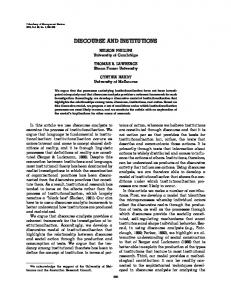
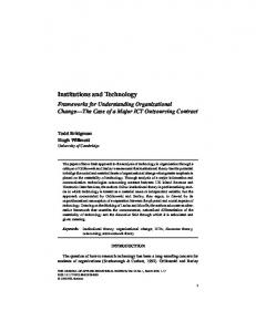
rates higher, in the poorer countries than in the more affluent ones. The same is true of the composition of crime, as viewed by the victims themselves, between serious and light crime. The nature and magnitude of association between crime and bribery is depicted in Figures 1-3. They plot the scatter points representing a combination of average bribe and crime rates for a particular country, and draw the Lowess Plots based on the scatters. While Figure 1 shows the association between crime (overall) and bribery rates across countries, Figures 2 and 3 show, respectively, the corresponding association between serious crime and bribery rates , and light crime and bribery rates. The association between serious crime and bribery rates is positive and stronger than that between light crime and bribery rates. It is worth noting that while serious crime rates tend to increase monotonically with bribery rates, the light crime rates have a non monotonic relationship with bribery rates. The asymmetric pattern between serious and light crime is also seen from Figures 4-6 which show, respectively, the relationship between crime rates, serious crime rates and light crime rates and per capita GNP at PPP. As the country gets richer and enjoys higher living standards, the serious and (overall) crime rates both come down, but the light crime rates increase and register a mild decrease only at higher levels of per capita GNP. Figure 7 highlights the discussion by presenting the three graphs in the same Figure without the scatter points. The corresponding relation between bribery and GNP is depicted in Figure 8 which shows that, similar to serious crime rates, bribery rates decline as a country enjoys higher living standards. It is worth noting that the association between serious crime and GNP is very close to that between bribery and GNP in both magnitude and direction. As a further comparison, Figure 9 plots the bribe to crime ratio against GNP and finds a fairly strong negative relationship. As a country gets richer, the number of bribe cases goes down much faster than the number of crime cases so that their ratio declines quite rapidly. A poorer country not only experiences higher bribe and crime rates, the seriousness of the crimes increase there as well. 10   

The distribution of countries with respect of crime (overall), serious crime, light crime and bribes are presented for each sweep as kernel density plots in Figures10-13, respectively. We present below each figure the principal summary statistics of the corresponding kernel density graph. Due to insufficient number of observations, we did not calculate the country averages or draw the graphs for bribery in the first sweep .The median values show that, during the period considered, serious crime and bribery rates have both gone down sharply. The incidence of serious crime and crime (overall) increased marginally during the first half of the 1990s and then declined quite sharply during the late 1990s and the early part of the new millennium. In contrast, the light crime rates have been fairly static. Figure 13 and the summary measures below that figure show that there was a continuous and sharp decrease in the incidence of bribery during the latter half of the 1990s. The overall message from these figures is that as the transition economies and the poorer developing countries after a period of sluggishness in the early 1990s saw a significant increase in their living standards, their crime and bribe rates declined during the latter half of the 1990 s and beyond in the new millennium. The composition of crime shifted towards “light crime” away from “serious crime” as viewed by the victims themselves. The relation between bribe and growth rates has attracted much discussion in the corruption literature with Mauro (1995)’s result of a negative association between the two rates triggering a large literature. In contrast, there is no evidence or discussion of any association between crime and growth rates in the crime literature. One would also expect a negative relationship here since the forces that cause high bribery rates to lower growth by reducing investment (both domestic and foreign) are similar to those that should cause higher crime rates to undermine business confidence and hence constrain economic growth. Figure 14 presents evidence on this by plotting the 4 graphs in one figure. Consistent with the result presented in Svensson (2005) and Chatterjee and Ray (2009), we find no evidence of the celebrated strong and uniformly negative

11   

relationship, due to Mauro (1995), between corruption and growth rates12. This paper extends the result to find a similar absence of a strong negative relationship between crime and growth rates. The correlation magnitudes confirm the lack of a strong association between both corruption and growth rates and between crime and growth rates. Serious crime and crime (overall) have a negative association with growth only for countries with high crime rates, i.e. crime rates in excess of 0.5. Such countries exhibit a negative relationship between serious crime and growth rates. The graphs indicate that, over the ranges of the crime/corruption rates that prevail in the more affluent countries (i.e. corruption rates between 0.0 and 0.3, and light crime rates between 0.0 and 0.4) corruption and light crime act as a greater constraint on growth rates than serious crime. The overall message from these graphs, namely, Figures 7, 8 and 14, is as follows. We do not find overwhelming evidence that either corruption or crime has a strong association with growth rates that is uniformly negative at all values of crime and corruption rates. The limited evidence that does emerge from these graphs is that for poorer countries (i.e. typically those with per capita GNP less than $20000), serious crime and crime (in general) have a negative impact on growth. As a country develops and living standards improve and crime rates drop, light crime and corruption take over as significant impediments to growth. The range of per capita GNP between $20,000 and $30,000 is the dividing range where the constraint on growth shifts from serious crime to corruption and light crime.

4.

The Determinants of Crime and Corruption

The probit regression estimates of crime and corruption on a selection of individual and country characteristics have been presented in the two halves of Table 1. This Table also presents the                                                              12

The OLS estimates presented later show, however, that corruption impacts significantly and nonlinearly on growth rates. Consistent with the backward bending curve in Figure14 showing the relationship between growth and corruption rates, the OLS estimates suggest that at very low levels of corruption, it impacts positively on growth rates but as one crosses a threshold corruption rate of around 0.16 or 16 %, it impacts negatively on growth.  

12   

corresponding probit coefficient estimates for serious crime rates. The corresponding marginal effects have been reported in Table 2. There are some interesting similarities between the effects of the various individual and country characteristics on an individual’s exposure to crime, serious crime and corruption victimisation. The size of a town’s population has strong and similar effects on both crime and bribery. Residents of a large town (the default category), i.e. one with a population size of more than 1 million people, are more likely to witness both crime and corruption than those in less populated places. Hunt (2006)’s explanation of this result in the corruption context, through the formation of informal net works in the smaller towns and cities as anti corruption mechanisms, holds for crimes as well. In the larger towns and cities, such networks that act as protective mechanisms are more difficult to form making the individual more vulnerable to both crime and bribe demands. The gender effects differ in both sign and significance between the two forms of victimisation. Males are more likely to be approached with bribe offers than females but females are more prone to being crime victims than males. The weak statistical significance of the effect of gender on crime victimisation contrasts sharply with the strong significance of gender effect on bribe victimisation. Note also that the gender effect on serious crime victimisation is much stronger in both size and significance than non serious or light crime. With increasing age, individuals are less exposed to both crime and bribery. Individuals in the oldest age category, 60 years and above, are least exposed to both crime and bribery compared to those in the default age group of less than 35 years. Married individuals are less likely than non married individuals to be crime victims, but the reverse is true in case of corruption victimisation. Working men and women are less exposed to crimes but more exposed to corruption than non working individuals. The latter result is explained by the possibilities of corruption that open up due to work related contact. Individuals in the higher income brackets and the more educated ones are more likely to

13   

be victims of crime and bribery than those who are poorer and less educated13. Individuals who are crime victims also report greater approaches for bribes. This is consistent with the result of Hunt (2007) who suggests that a crime victim having reported the crime to the police comes in contact with potentially corrupt officials increasing her/his exposure to bribe demands. There are some interesting similarities and contrasts between the country effects on crime and bribery. The OLS results show that rising inequality reduces (overall) crime and bribery14 but increases serious crime15. The IV results presented below show however that rising inequality has a positive impact on bribery. A strengthening of the rule of law reduces both crime and corruption. Ceteris paribus, a happier16 society sees less of both crime, especially serious crime, and corruption. The only previous evidence of a link between happiness and crime victimisation, that we are aware of, is that of Powdthavee (2005) who found on South African data that “victims report significantly lower well-being than the non-victims” and that “happiness is lower for non-victimized respondents currently living in higher crime areas”(p.531). Powdthavee (2005)’ s study ,which complements the present study, looks at the link running from crime( cause) to unhappiness (effect) based on single country data while ours , based on cross country data, provides evidence on the link running from unhappiness (cause) to crime (effect).While rising unemployment has a strong positive effect on overall crime rates, but a negative effect on serious crime rates, it has no significant impact on corruption. Population size has a similar effect to that of unemployment in impacting positively on crime, negatively on serious crime and has no effect on corruption. Improvements in the human development indicator (HDI) lead, paradoxically, to a more crime prone but a less corrupt country. The time coefficients show that,                                                              13

This effect may reflect the fact that the educated and high income earners are more likely to record and report crime and corruption victimisation than the others.

See also Gupta, et. al. (2002) and Li, et. al. (2000) for evidence on the association between inequality and bribery. Note however that, as we report later, the effect of inequality on crime and bribery is sensitive to the relaxation of the exogeneity assumption and the use of IV. 16 See Oswald (1997) and Frey and Stutzer (2000) for evidence on the association between the subjective measures of individual well being and a host of demographic, economic and institutional variables.     14 15

14   

once individual and country effects are controlled, there was a decrease in the serious crime rates. The probit estimates in Tables 1 are likely to suffer from bias if one or more of the country variables are correlated with variables that, also, influence the respondent’s answers to the questions on crime and bribe victimisation .The issue of sensitivity of the principal results to the relaxation of the OLS assumptions is examined by reporting the IV probits of crime, serious crime and bribe in Table 3.The country variables, regulatory burden, HDI and unemployment rate were treated as potentially endogenous and instrumented by Freedom of Press, Economic Freedom and Female/Male ratio which are all available at the country level. The Wald test easily rejects the assumption of exogeneity underlying the probit estimates of Table 1. A comparison of Tables 1 and 3 confirms, however, that, qualitatively, the effects of the individual characteristics on crime and corruption are fairly robust between the two sets of probit estimates. For example, residents of the larger towns and cities continue to report more crime and bribe victimisation, males report more bribe demands, females report more incidents of crime and serious crime victimisation. While with increasing age, individuals are less exposed to crime and bribe victimisation, with increasing education and income, individuals are more exposed to both types of victimisation. The earlier result that crime victims are more likely than non victims of crime to be approached for bribes holds in the presence of IV probit estimation as well. The country effects are less robust between the ordinary probit estimates reported in Table 1 and the IV probit estimates reported in Table 3. Rising unemployment increases both crime and bribery, while improvement in the human development indicator also leads, paradoxically, to an increase in both forms of victimisation. This latter, somewhat paradoxical, result may be explained by the fact that with an improvement in the human development indicator, residents are more likely to be forthcoming in reporting both crime and corruption. A strengthening of the legal institutions, as measured by the rule of law variable (rol), leads to a decline in crime and in 15   

bribery. A happier society sees less of both crime and bribery. These results, that establish the positive roles that the quality of legal system and happiness can play in reducing crime and corruption in society, acquire significance in view of their robustness between the probit and the IV probit estimates. Table 3 shows that rising inequality increases serious crimes and corruption. The IV estimates show that, once individual and country characteristics are controlled, there was a significant decline in crime and in bribery. This is consistent with the summary statistics presented and discussed in Section 3. The decline was particularly sharp in case of corruption followed by serious crime. In the spirit of this exercise that looks at the possible nexus between crime and corruption, we performed ordered probit estimation where the following outcomes, based on combinations of crime and bribe victimisation, were defined and ordered sequentially with a higher order denoting a superior outcome. (1) Respondent reports being a victim of both crime and bribery (i.e. Crime=1, Bribery=1). (2) Respondent reports either crime victimisation or bribe victimisation, but not both (Crime=1, Bribery=0, or Crime=0, Bribery=1). (3) Respondent denies being a victim of either crime or bribery (Crime=0, Bribe=0). Clearly the third outcome is the best, the first the worst, with (2) being the intermediate one. The ordered probit estimates (without and with the country effects) have been presented in Table 4. Keeping in mind the possibility of non linearities in the relationship between inequality and crime/corruption, we allow both linear and square terms in the inequality variable in the ordered probit regressions. If statistically significant, a positive sign of the estimated coefficient indicates a move towards a superior outcome, a negative sign otherwise, when the relevant characteristic increases by one unit. A comparison between the two halves of Table 4 confirms that the qualitative impact of the respondent’s individual characteristics to the combination of crime and 16   

bribe victimisation that she/he reports is robust to the introduction of the country indicators. Ceteris paribus, residents of smaller sized towns and cities, females, older adults, lower income earning individuals and less educated individuals are more likely report the superior outcome of no bribe and no crime victimisation. The country effects are also in line with the earlier results. For example, while stronger legal institutions, as measured by Rule of Law (rol) , and increasing happiness push the country towards a superior outcome, rising unemployment and an increase in the regulatory burden contribute to an inferior outcome. The inverse U shaped impact of inequality is interesting - initially, inequality pushes the country towards a superior outcome, but high inequality does the reverse. There are strong regional effects as well. Residents of countries in East Asia and the Pacific are better off than those in Europe and the Caribbean, while those in Latin America fare the worst. The Latin Americans are the most exposed to both crime and corruption victimisation. Consistent with the earlier evidence, as reported in the summary statistics and the probit regression estimates, the significantly positive estimate of the time trend confirms that over the period of this study, the world has moved towards the best outcome, i.e., has become a safer place from the viewpoint of both crimes and bribery.

5.

Impact of Crime and Corruption on Growth

This section shifts attention from the determinants of crime and corruption to their effects on a country’s growth rate. As we mentioned earlier, the resurgence of interest in the corruption literature was triggered by Mauro (1995)’s result that corruption impacts negatively on growth by reducing investment. This result has been found to lack robustness in subsequent studies, including Mauro’s own study on cross country data using the Business International (BI) Index of corruption17. The present study revisits the issue by providing evidence on the association between growth and corruption using the country means from the ICVS data on corruption. We also extend the literature by providing evidence, where currently none exists, on the relation                                                              17

Apart from the fact that the BI data is subjective and is based on perceptions, it is an ordinal measure though it has been treated as cardinal in most of the studies that are based on this data set. This is also true of studies that use the perceptions data from the Transparency International.

17   

between crime and growth rates and, further, on that between serious crime and growth rates. In common with the rest of the study, we provide evidence on robustness by presenting OLS and IV estimates of the regressions. The OLS, IV regression estimates of crime, serious crime and corruption, along with a selection of country level variables, on a country’s growth rate are presented in Tables 5 and 6 respectively. In the IV estimations, we instrumented the principal determinants of interest, namely, crime, serious crime and bribery rates (and their squares) by a selection of variables that include economic freedom, freedom of press, government intervention, informal sector, government control of wages and prices, and happiness. Since the country level variables, that were collected from a variety of sources listed in the Appendix (Table A2)18, were not available for all the countries in the ICVS data set, a significant consideration behind the choice of those to include in the regressions was their availability for as many countries as possible, so as to not lose too many observations. The IV estimates confirm the validity of the instruments. The OLS estimates presented in table 5 show that corruption does impact nonlinearly on growth rates with the coefficients of the linear corruption rate variable and the square of corruption rate variable recording statistical significances at 5% level of significance. The estimated magnitude of the coefficients of the linear and square terms show that at low levels, corruption impacts positively on growth, but as the corruption rate exceeds a threshold of around 16 %, it starts to impact negatively on growth. Table 6 shows, however, that the effect of corruption on growth weakens to insignificance on the use of IV estimation. In case of crime, neither crime rates nor serious crime rates have significant effects on growth rates and this result holds true in case of both OLS19 and IV estimates .This lack of a strong association between crime and growth rates and between corruption and growth rates is consistent with the picture portrayed in Figure 14 and                                                              18

See Appendix Table A2 for a full listing of all the variables (with their abbreviated names), along with the sources, used in this study.  19 The OLS estimates show that serious crime has a marginally stronger negative impact on growth than does crime (overall) via the significance, at 10 % level of significance, of the square term in serious crime rate in Table 5.

18   

the weak correlation magnitudes reported there. The OLS estimates show that, ceteris paribus, the strengthening of legal institutions that is captured by the rule of law variable leads to an increase in the growth rate. This effect weakens somewhat in case of IV estimation.

6.

Summary and Conclusions

This paper uses a large cross country micro data set (ICVS) to compare the determinants of crime and bribe victimisation and their effects on economic growth. This data set contains information on both forms of victimisation in a range of countries that span a wide spectrum of economic and social indicators. The paper exploits a unique feature of the data set that the same individual was asked whether she/he was a crime and a bribe victim. The responses contained in the data set are accompanied by the individual characteristics of the respondent. The study uses the crime victim’s own subjective view to categorise the crime committed into “serious crime” and “non serious or light crime”. The study supplements the individual characteristics with country level information obtained from a variety of sources to examine the effect of individual characteristics and institutions in the respondent’s country of residence on the individual’s exposure to crime and corruption. This paper also contains evidence on the association between crime and corruption at both country level and at the level of individuals. A methodological novelty of this study is the ordered probit estimation where combinations of crime and bribe victimisation were used to define and order outcomes in a welfare improving ascending order. This study also examines the question whether crime impacts negatively on a country’s growth rate similar to the result on corruption that generated a large literature. The principal results include the evidence that suggests that while males are more vulnerable to bribe demands, females are more likely to be crime victims, especially of serious crime. The role of informal social networks in the smaller towns and cities in acting as protective mechanisms against crime and bribe victimisation explains the higher prevalence of both forms of victimisation in the more populated regions. A crime victim is more likely to be exposed to bribe 19   

demands than a non victim. Rising income and higher education levels increase the individual’s exposure to both crime and bribery. The paper contains evidence on the importance of institutions and country level indicators in explaining cross country differences in the individual’s exposure to both forms of victimisation. For example, the strengthening of the rule of law reduces the incidence of both crime and corruption. A happier country also sees less of both crime and corruption. The paper also contains evidence that rising unemployment and inequality lead to higher criminalisation and a more corrupt society. The last two results are not unrelated since, as Frey and Stutzer (2000) observe, “unemployment has a strongly depressing effect on happiness”20. It is also important to recognise the lack of robustness of some of the country level determinants of crime and corruption between the OLS and IV regression results. The most prominent of these is the effect of inequality on crime and corruption. This may point to the need to allow for the mutual impact of corruption and inequality on one another, as You and Khagram (2005) suggest, but such an extension is beyond the scope of this study. Against such a background of non robustness of several country effects21, the robust evidence on the positive role of rule of law and happiness in reducing both forms of victimisation is a result of considerable significance. The ordered probit estimates establish the robustness of the positive role that a strengthened legal system and a happier society play in improving outcomes. This study finds no strong evidence of any significant association either between crime and growth rates or between corruption and growth rates. While the former result is found to be robust to the treatment of endogeneity and the use of IV estimation, the OLS estimates provide limited evidence that suggests that corruption impacts nonlinearly on growth rates. At low levels, corruption has a positive effect on growth, but impacts negatively at higher levels of corruption.                                                              20

See also Oswald (1997) for strong evidence of the negative association between unemployment and happiness or, as he says, “unemployed people are very unhappy”. 21 The lack of robustness of several of the country effects possibly reflects the inferior quality of the country level indicators, especially the lack of a consistent time series of such information to coincide with the time period of the ICVS data sets, and the consequent problem of errors in variables that this entails.    

20   

This evidence of a significant effect of corruption on growth rate disappears on the use of IV estimation. A by product of this exercise is the evidence on the positive role that the strengthening of legal institutions plays in increasing a country’s growth rate. This study was motivated by an attempt to bridge the gap between the parallel literatures on crime and corruption. While the evidence on the determinants of crime and corruption are of interest on their own, the focus of this study has been on a comparison between their magnitudes, determinants and effects on growth. The results of this study point to the importance of both individual characteristics and institutions in profiling an individual who is at a high risk from both crime and bribery. As we gain access to more data sets that contain information on crime and corruption, the recent convergence in the two empirical literatures will gather momentum. The results of this exercise suggest that examination of the link between crime and corruption and attempts to integrate studies of the two types of victimisation provide a fruitful area for further research. The estimates of the effect of unemployment and inequality on crime and corruption and their non robustness to the use of IV estimation seem to suggest a more complex relationship than we have considered in this study. The simultaneous estimation of crime, corruption, inequality and unemployment incorporating their mutual dependence is another fruitful area for further research that is indicated by the present results. A result that stands out because of its robustness is the role of rising happiness in reducing both crime and corruption in society. The present study suggests that it plays an analogous role to that of legal institutions in checking crime and corruption. In recent years, as the study by Frey and Stutzer (2000) illustrates, economists have been paying increasing attention to happiness and its determinants. Much of the literature on happiness, summarised in Oswald (1997), has been on its magnitude and determinants rather than on its consequences for outcomes such as crime and corruption. The present results suggest that we need to change focus from the former to the 21   

latter. To our knowledge there has not been any previous attempt to study the link between happiness, crime and corruption. While there is now an emerging literature on the link between crime and happiness [Powdthavee (2005)] and on the link between crime and corruption [Hunt (2007)], there has been no previous attempt to examine the link between crime, corruption and happiness in a unified framework .A greater exploration of the link between happiness (at both individual and country levels), institutions, crime and corruption provides another fertile ground for further research. For such a study to proceed, we need more and better quality data on institutions that are consistently available for a large number of countries over a long time period. Given the importance of institutions in explaining cross country differences in crime and corruption, as this study has demonstrated, the need to embark on a project to collect such information on an international scale comparable to the ICVS data sets that have been used here cannot be overstated.

References Bardhan, P. (1997), “Corruption and Development: A Review of Issues”, Journal of Economic Literature, 35, 1320-1346. Baum, C.F., Schaffer, M.E., and Stillman, S. (2007), “Ivreg2: Stata module for extended instrumental variables/2SLS, GMM and AC/HAC, LIML and k-class regression”, http://ideas.repec.org/c/boc/bocode/s425401.html Becker, G.S. (1968), “Crime and Punishment: An Economic approach”, Journal of Political Economy, 76 (2), 169-217. Buonanno, P. (2003), “The Socioeconomic Determinants of Crime: A Review of the Literature”, Working paper No. 63 of Dipartimento di Economia Politica, Universita degli Studi di MilanoBicocca, November. Cameron, S. (1988), “The Economics of Crime Deterrence: A Survey of Theory and Evidence”, Kyklos, 41(2), 301-323. Chatterjee, I. and Ray, R. (2009), “Does the Evidence on Corruption Depend on how it is measured? Results from a Cross Country Study on Micro Data sets”, Discussion paper 07-09 of 22   

Department of Economics, Monash University, Melbourne, Discussion Paper Series (http://www.buseco.monash.edu.au/eco/research/papers/2009/0709corruptionchatterjeeray.pdf). Dabla-Norris, E., Gradstein, M., and Inchauste, G. (2008), “What causes firms to hide output? The determinants of informality”, Journal of Development Economics, 85, 1-27. Djankov, S., La Porta, R., Lopez-de-Silanes, F., and Shleifer, A. (2002), “The regulation of entry”, Quarterly Journal of Economics, 117, 1-37. Ehrlich, I. (1973), “Participation in Illegitimate Activities: A Theoretical and Empirical Investigation”, Journal of Political Economy, 81, 521-565. Ehrlich,I. (1981), “On the usefulness of Controlling Individuals: An Economic Analysis of Rehabilitation, Incapacitation and Deterrence”, The American Economic Review, 71(3), 307-322. Fajnzylber, P., Lederman, D. and Loayza, N. (2002), “What causes violent crime?”, European Economic Review, 46, 1323-1357. Frey, B.S. and Stutzer, A. (2000), “Happiness, Economy and Institutions”, The Economic Journal, 110, 918-938. Grogger, J. (1991), “Certainty vs. Severity of Punishment “, Economic Inquiry, 29, 297-309. Gupta, S., Davoodi, H. and Alonso-Terme, R. (2002), “Does Corruption affect income inequality and poverty?”, Economics of Governance, 3, 23-45. Hunt, J. (2006), “How Corruption hits people when they are down”, NBER Working Paper, No. 12490. Hunt, J. (2007), “How Corruption hits people when they are down”, Journal of Development Economics, 84, 574-589. Jain, A. (2001), “Corruption: A Review”, Journal of Economic Surveys, 15(1), 71-121. Kelly, M. (2000), “Inequality and Crime”, The Review of Economics and Statistics, 82 (4), 530539. Levitt, S. (1998), “Why do increased arrest rates appear to reduce crime: deterrence, incapacitation, or measurement error?”, Economic Inquiry, 36, 353-372. Li, H., Xu, X.C., and Zou, H. (2000), “Corruption, Income Distribution and Growth”, Economics and Politics, 12(2), 155-182. 23   

Mauro, P. (1995), “Corruption and Growth”, Quarterly Journal of Economics, 110, 681-712. Mendez, F. and Sepulveda, F. (2006), “Corruption, growth and political regimes: cross country evidence”, European Journal of Political Economy, 22, 82-98. Mishra, A. (2005), The Economics of Corruption, Oxford University Press, New Delhi. Mocan, N. (2008), “What determines Corruption? International Evidence from Corruption data”, Economic Inquiry, 46(4), 493-510. Myers, S.L. (1983),”Estimating the Economic Model of Crime: Employment Versus Punishment Effects”, The Quarterly Journal of Economics, 98(1), 157-166. Myrdal, G. (1968), Asian Drama: An Inquiry into the Poverty of Nations, Pantheon, New York. Oswald, A.J. (1997), “Happiness and economic performance”, Economic Journal, 107 (445), 1815-1831. Paldam, M. (2002), “The cross-country pattern of corruption: economics, culture and the seesaw dynamics”, European Journal of Political Economy, 18, 215-240. Powdthavee, N. (2005), “Unhappiness and Crime: Evidence from South Africa”, Economica, 72, 531-547. Stigler, G. (1970), “The Optimum Enforcement of Laws”, Journal of Political Economy, 78(2), 526-536. Svensson, J. (2003), “Who must pay bribes and how much: evidence from a cross section of firms”, Quarterly Journal of Economics, 118(1), 207-230. Svensson, J. (2005), “Eight Questions about Corruption”, Journal of Economic Perspectives, 19(3), 19-42. Treisman, D. (2000), “The causes of corruption: a cross-national study”, Journal of Public Economics, 76, 399-457. Witte, A.D. (1980), “Estimating the Economic Model of Crime with Individual Data”, The Quarterly Journal of Economics, 94(1), 57-84. Wolpin, K.I. (1980), “A Time Series-Cross Section Analysis of International Variation in Crime and Punishment”, The Review of Economics and Statistics, 62(3), 417-423. 24   

You, J. and Khagram, S. (2005), “A Comparative Study of Inequality and Corruption”, American Sociological Review, 70, 136-157.

25   

Figures: Figure 1: Lowess Fit between Crime and Bribe Rates, 1991 - 2005

Figure 2: Lowess Fit between Serious Crime and Bribe Rates, 1991 - 2005

Figure 3: Lowess Fit between Light Crime and Bribe Rates, 1991 - 2005 26   

Figure 4: Lowess Fit between per capita GNP at PPP and Crime Rate, 1991 - 2005

Figure 5: Lowess Fit between per capita GNP at PPP and Serious Crime Rate, 1991 - 2005

27   

Figure 6: Lowess Fit between per capita GNP at PPP and Light Crime Rate, 1991 - 2005

Figure 7: Lowess Fit between per capita GNP at PPP and the three Crime Rates, 1991 - 2005

28   

Figure 8: Lowess Fit between per capita GNP at PPP and Bribe Rate, 1991 - 2005

Figure 9: Lowess Fit between per capita GNP at PPP and Bribe to Crime Ratio, 1991 - 2005

29   

30   

Figure 10: Crime Rate Distributions − Kernel Densities for 1991, 1995, 1999 and 2003

variable crime rate 91 crime rate 95 crime rate 99 crime rate 03

N 29 44 46 34

mean 0.711 0.679 0.665 0.537

max 1.000 0.946 1.000 1.000

min 0.409 0.336 0.316 0.261

sd 0.163 0.123 0.166 0.150

variance median skewness kurtosis 0.026 0.649 0.440 2.174 0.015 0.663 -0.119 3.335 0.028 0.696 -0.017 2.217 0.022 0.515 1.499 6.437

Figure 11: Serious Crime Rate Distributions − Kernel Densities for 1991, 1995, 1999 and 2003 31   

variable SCR91 SCR95 SCR99 SCR03

N 29 44 46 34

mean 0.596 0.573 0.549 0.396

max 0.990 0.876 0.925 0.665

min 0.332 0.267 0.233 0.210

sd 0.186 0.151 0.176 0.099

variance median skewness kurtosis 0.035 0.545 0.550 2.167 0.023 0.566 0.101 2.353 0.031 0.561 0.069 1.848 0.010 0.399 0.583 3.968

Figure 12: Light Crime Rate Distributions − Kernel Densities for 1991, 1995, 1999 and 2003

32   

variable LCR91 LCR95 LCR99 LCR03

N 29 44 46 34

mean 0.115 0.106 0.116 0.142

max 0.256 0.222 0.516 0.600

min 0.005 0.037 0.000 0.004

sd 0.066 0.047 0.082 0.100

variance median skewness kurtosis 0.004 0.119 0.187 2.461 0.002 0.096 0.703 2.759 0.007 0.100 2.643 13.347 0.010 0.118 3.087 14.485

Figure 13: Bribe Rate Distributions − Kernel Densities for 1995, 1999 and 2003

33   

variable bribe rate 95 bribe rate 99 bribe rate 03

N 44 44 33

mean 0.107 0.105 0.032

max 0.302 0.591 0.155

min 0.001 0.000 0.000

sd 0.090 0.118 0.046

variance median skewness kurtosis 0.008 0.102 0.567 2.360 0.014 0.072 1.823 7.714 0.002 0.006 1.416 3.606

Figure 14: Lowess Fit between Growth and Bribe Rates, and between Growth and Crime Rates, 1991 - 2005

34   

35   

Tables: Table 1: Probit Coefficient Estimates of Crime and Corruption, 1991-2005 Variablesb Coefficient

c

Crimea Robust SE

z

P>|z|

c

Coefficient

Serious Crimea Robust SE z

P>|z|

Bribe or Corruptiona Coefficient Robust SE z c

P>|z|

smalltown -0.270* 0.015 -18.06 0.000 -0.161* 0.021 -7.85 0.000 -0.255* 0.030 -8.52 0.000 medtown -0.067* 0.016 -4.14 0.000 -0.034 0.022 -1.5 0.134 -0.196* 0.028 -6.96 0.000 male -0.021*** 0.011 -1.87 0.061 -0.160* 0.015 -10.45 0.000 0.318* 0.021 15.37 0.000 age35to60 -0.140* 0.014 -9.67 0.000 0.024 0.019 1.27 0.205 -0.172* 0.024 -7.24 0.000 ageabove60 -0.452* 0.022 -20.32 0.000 -0.086* 0.031 -2.76 0.006 -0.455* 0.048 -9.43 0.000 married -0.043* 0.012 -3.59 0.000 -0.064* 0.017 -3.83 0.000 0.066* 0.023 2.83 0.005 working -0.121* 0.037 -3.26 0.001 0.019 0.042 0.45 0.653 0.116** 0.057 2.03 0.042 lookwork -0.220* 0.041 -5.33 0.000 -0.001 0.048 -0.03 0.979 0.071 0.063 1.12 0.263 homekeeper -0.280* 0.041 -6.79 0.000 -0.018 0.050 -0.35 0.726 0.100 0.069 1.45 0.148 retired -0.270* 0.040 -6.73 0.000 0.022 0.047 0.46 0.642 -0.121*** 0.069 -1.76 0.079 at school -0.251* 0.047 -5.31 0.000 -0.099*** 0.055 -1.79 0.073 0.027 0.067 0.4 0.690 upperincome 0.146* 0.012 12.23 0.000 -0.040** 0.016 -2.51 0.012 0.095* 0.021 4.52 0.000 education years 0.034* 0.002 18.07 0.000 0.012* 0.002 5.42 0.000 0.027* 0.003 10.16 0.000 crime 0.513* 0.027 18.94 0.000 t 0.033** 0.016 2.11 0.035 -0.395* 0.021 -18.64 0.000 0.085* 0.022 3.86 0.000 hdi 3.891* 0.420 9.26 0.000 1.766* 0.602 2.93 0.003 -4.616* 0.667 -6.92 0.000 rol -0.327* 0.027 -12.06 0.000 0.060 0.039 1.54 0.123 -0.319* 0.040 -7.92 0.000 reg1000 0.871* 0.133 6.56 0.000 0.532** 0.214 2.48 0.013 -1.844* 0.187 -9.85 0.000 unemployment 0.043* 0.002 27.24 0.000 -0.037* 0.002 -18.42 0.000 -0.002 0.002 -0.76 0.447 inequality -0.005* 0.002 -2.87 0.004 0.016* 0.003 5.92 0.000 -0.030* 0.003 -9.2 0.000 happy_ls10 -0.006 0.016 -0.4 0.686 -0.250* 0.019 -12.82 0.000 -0.251* 0.019 -13.47 0.000 lpop 0.035* 0.007 4.69 0.000 -0.089* 0.010 -8.5 0.000 -0.006 0.012 -0.5 0.619 Deap -0.779* 0.056 -13.91 0.000 -0.124 0.081 -1.54 0.124 0.484* 0.092 5.27 0.000 Deuca 0.103* 0.025 4.07 0.000 -0.033 0.037 -0.89 0.376 0.063 0.075 0.84 0.398 Dla 0.662* 0.057 11.69 0.000 0.510* 0.071 7.15 0.000 1.183* 0.077 15.35 0.000 constant -2.456* 0.282 -8.71 0.000 2.593* 0.403 6.43 0.000 5.598* 0.422 13.27 0.000 No. of obs 60021 36356 60003 Log Pseudolikelihood -36371.657 -19009.657 -9576.0755 Pseudo R2 0.0964 0.0937 0.2225 a. Equals to 1 if a victim, 0 otherwise. b. See Appendix Table A2 for meaning of the variable names. c. *, ** and *** imply significance at 1%, 5% and 10% levels.

36   

Table 2: Marginal Effects of Individual, Country and Institutional Characteristics on Crime and Corruption, 1991-2005 Variablesb dy/dx

Crimea Std Error

z

P>|z|

dy/dx

Serious Crimea Std Error z

P>|z|

dy/dx

Bribe or Corruptiona Std Error z

P>|z|

smalltown # -0.103* 0.006 -18.08 0.000 -0.051* 0.007 -7.77 0.000 -0.011* 0.001 -8.47 0.000 medtown # -0.026* 0.006 -4.12 0.000 -0.011 0.007 -1.49 0.136 -0.008* 0.001 -7.43 0.000 male # -0.008*** 0.004 -1.87 0.062 -0.050* 0.005 -10.4 0.000 0.015* 0.001 14.26 0.000 age35to60 # -0.053* 0.006 -9.67 0.000 0.007 0.006 1.27 0.204 -0.007* 0.001 -7.21 0.000 ageabove60 # -0.176* 0.009 -20.23 0.000 -0.027* 0.010 -2.71 0.007 -0.016* 0.001 -11.61 0.000 married # -0.017* 0.005 -3.6 0.000 -0.020* 0.005 -3.84 0.000 0.003* 0.001 2.85 0.004 working # -0.046* 0.014 -3.27 0.001 0.006 0.013 0.45 0.653 0.005** 0.003 2.03 0.042 lookwork # -0.086* 0.016 -5.25 0.000 0.000 0.015 -0.03 0.979 0.003 0.003 1.05 0.293 homekeeper # -0.109* 0.016 -6.69 0.000 -0.006 0.016 -0.35 0.727 0.005 0.004 1.33 0.184 retired # -0.104* 0.016 -6.67 0.000 0.007 0.015 0.47 0.641 -0.005*** 0.003 -1.86 0.063 at school # -0.098* 0.019 -5.22 0.000 -0.032*** 0.018 -1.74 0.081 0.001 0.003 0.39 0.697 upperincome # 0.055* 0.005 12.3 0.000 -0.013** 0.005 -2.51 0.012 0.004* 0.001 4.45 0.000 education years 0.013* 0.001 18.1 0.000 0.004* 0.001 5.42 0.000 0.001* 0.000 9.95 0.000 crime # 0.021* 0.001 20.64 0.000 t 0.013** 0.006 2.11 0.035 -0.124* 0.007 -18.8 0.000 0.004* 0.001 3.87 0.000 hdi 1.483* 0.160 9.26 0.000 0.552* 0.188 2.94 0.003 -0.202* 0.029 -6.96 0.000 rol -0.125* 0.010 -12.06 0.000 0.019 0.012 1.54 0.123 -0.014* 0.002 -7.73 0.000 reg1000 0.332* 0.051 6.56 0.000 0.166** 0.067 2.48 0.013 -0.081* 0.008 -9.71 0.000 unemployment 0.016* 0.001 27.25 0.000 -0.012* 0.001 -18.5 0.000 0.000 0.000 -0.76 0.447 inequality -0.002* 0.001 -2.87 0.004 0.005* 0.001 5.93 0.000 -0.001* 0.000 -9.01 0.000 happy_ls10 -0.002 0.006 -0.4 0.686 -0.078* 0.006 -12.88 0.000 -0.011* 0.001 -12.79 0.000 lpop 0.013* 0.003 4.69 0.000 -0.028* 0.003 -8.49 0.000 0.000 0.001 -0.5 0.619 Deap # -0.303* 0.020 -14.89 0.000 -0.040 0.027 -1.48 0.138 0.033* 0.009 3.66 0.000 Deuca # 0.040* 0.010 4.04 0.000 -0.010 0.011 -0.89 0.372 0.003 0.003 0.89 0.376 Dla # 0.218* 0.015 14.58 0.000 0.133* 0.015 8.98 0.000 0.149* 0.018 8.27 0.000 a. Equals to 1 if a victim, 0 otherwise. b. See Appendix Table A2 for meaning of the variable names. c. *, ** and *** imply significance at 1%, 5% and 10% levels. (#) dy/dx is for discrete change of dummy variable from 0 to 1.

37   

Table 3: IV-Probit Coefficient Estimates of Crime and Corruption, 1991-2005 Variables

b

Coefficient

c

Crimea Robust SE

z

P>|z|

Serious Crimea Coefficient Robust SE z c

P>|z|

Bribe or Corruptiona Coefficientc Robust SE z

reg1000 -1.205* 0.414 -2.91 0.004 1.877* 0.612 3.07 0.002 3.387* hdi 14.895* 3.560 4.18 0.000 12.889* 3.784 3.41 0.001 60.468* unemployment 0.042* 0.015 2.76 0.006 0.019 0.019 1.04 0.299 0.280* smalltown -0.301* 0.017 -17.37 0.000 -0.211* 0.026 -8.13 0.000 -0.434* medtown -0.110* 0.019 -5.81 0.000 -0.068* 0.025 -2.73 0.006 -0.368* male -0.028** 0.012 -2.4 0.016 -0.163* 0.016 -10.41 0.000 0.280* age35to60 -0.148* 0.015 -9.91 0.000 0.036*** 0.019 1.84 0.066 -0.126* ageabove60 -0.490* 0.023 -21.58 0.000 -0.072** 0.032 -2.23 0.026 -0.472* married -0.041* 0.013 -3.2 0.001 -0.076* 0.017 -4.37 0.000 -0.009 working -0.151* 0.039 -3.83 0.000 0.042 0.044 0.97 0.332 0.214* lookwork -0.216* 0.043 -5 0.000 -0.021 0.050 -0.43 0.669 0.044 homekeeper -0.328* 0.043 -7.63 0.000 -0.004 0.052 -0.07 0.942 0.108 retired -0.257* 0.043 -5.95 0.000 0.051 0.050 1.03 0.303 0.066 at school -0.255* 0.049 -5.25 0.000 -0.090 0.056 -1.61 0.107 0.001 upperincome 0.173* 0.017 10.23 0.000 0.000 0.021 0 0.997 0.328* education years 0.030* 0.002 16.87 0.000 0.010* 0.002 3.98 0.000 0.018* crime 0.245* t -0.277** 0.122 -2.27 0.023 -0.819* 0.142 -5.78 0.000 -2.128* rol -0.954* 0.115 -8.3 0.000 -0.285** 0.126 -2.26 0.024 -2.445* inequality -0.004 0.005 -0.87 0.384 0.033* 0.007 4.79 0.000 0.044* happy_ls10 -0.294* 0.039 -7.44 0.000 -0.286* 0.028 -10.3 0.000 -0.912* lpop 0.075* 0.011 7 0.000 -0.126* 0.019 -6.8 0.000 -0.034*** Deap 0.336*** 0.186 1.81 0.070 0.293*** 0.163 1.8 0.072 3.469* Deuca 0.112* 0.026 4.28 0.000 -0.003 0.039 -0.06 0.948 -0.062 Dla 0.993* 0.067 14.82 0.000 0.341* 0.096 3.54 0.000 1.415* constant -6.942* 2.364 -2.94 0.003 -5.079*** 2.606 -1.95 0.051 -37.381* No. of obs 60021 36356 Wald test of significance: χ2 (24) 6485.65 3059.43 Prob > χ2 0.0000* 0.0000* Wald test of exogeneity: χ2 (3) 332.68 10.89 Prob > χ2 0.0000* 0.0124** a. Equals to 1 if a victim, 0 otherwise. b. See Appendix Table A2 for meaning of the variable names. c. *, ** and *** imply significance at 1%, 5% and 10% levels.

0.828 7.581 0.032 0.038 0.038 0.024 0.028 0.053 0.027 0.067 0.074 0.079 0.081 0.080 0.036 0.003 0.041 0.256 0.246 0.010 0.082 0.018 0.366 0.084 0.100 5.044

4.09 7.98 8.84 -11.34 -9.7 11.67 -4.53 -8.83 -0.33 3.19 0.59 1.37 0.82 0.01 9.09 5.17 5.93 -8.32 -9.96 4.26 -11.08 -1.94 9.47 -0.74 14.15 -7.41

P>|z| 0.000 0.000 0.000 0.000 0.000 0.000 0.000 0.000 0.738 0.001 0.553 0.170 0.412 0.992 0.000 0.000 0.000 0.000 0.000 0.000 0.000 0.052 0.000 0.460 0.000 0.000 60003 2852.68 0.0000* 117.77 0.0000*

38   

Table 4: Ordereda Probit Coefficient Estimates of Crime and Corruption, 1991-2005 Variablesb

Coefficientc

Without Country Effects Robust SE z

P>|z|

Coefficientc

With Country Effects Robust SE z

P>|z|

smalltown 0.348* 0.007 49.35 0.000 0.279* 0.014 20.34 0.000 medtown 0.091* 0.008 11.1 0.000 0.107* 0.015 7.31 0.000 male -0.045* 0.006 -7 0.000 -0.054* 0.010 -5.15 0.000 age35to60 0.182* 0.008 23.29 0.000 0.150* 0.013 11.45 0.000 ageabove60 0.522* 0.012 42.3 0.000 0.456* 0.021 22.16 0.000 married 0.008 0.007 1.18 0.239 0.018 0.011 1.61 0.107 working 0.259* 0.020 12.85 0.000 0.024 0.030 0.81 0.420 lookwork 0.203* 0.023 8.73 0.000 0.118* 0.034 3.45 0.001 homekeepr 0.358* 0.022 16.21 0.000 0.161* 0.035 4.66 0.000 retired 0.352* 0.022 15.88 0.000 0.195* 0.033 5.89 0.000 at school 0.081* 0.027 3.04 0.002 0.140* 0.040 3.55 0.000 upperincome -0.175* 0.007 -26.46 0.000 -0.134* 0.011 -12.2 0.000 education years -0.020* 0.001 -22.6 0.000 -0.034* 0.002 -20.51 0.000 t 0.128* 0.004 33.82 0.000 0.032** 0.014 2.27 0.023 hdi -4.932* 0.432 -11.43 0.000 rol 0.386* 0.026 14.59 0.000 reg1000 -0.647* 0.129 -5.01 0.000 unemployment -0.035* 0.001 -23.55 0.000 inequality 0.061* 0.008 7.59 0.000 inequality squared -0.001* 0.000 -7.12 0.000 happy_ls10 0.102* 0.015 6.98 0.000 lpop -0.030* 0.007 -4.14 0.000 Deap 0.552* 0.054 10.24 0.000 Deuca -0.158* 0.024 -6.54 0.000 Dla -0.710* 0.050 -14.24 0.000 constant 2.100* 0.006 329.10 0.000 2.236* 0.011 205.69 0.000 No. of obs 153862 60003 Log Pseudolikelihood -120111.05 -44799.57 Pseudo R2 0.0563 0.1006 a. Order = 0, if crime = bribe=1; Order = 1 if crime=1, bribe=0 OR crime=0, bribe=1; Order = 2 if crime = bribe = 0. b. See Appendix Table A2 for meaning of the variable names. c. *, ** and *** imply significance at 1%, 5% and 10% levels.

39   

Table 5: OLS Coefficient Estimates of Growth Rates Dependent Variable: Growth Rate a

b

Variables

Coefficient Robust SE

t

Dependent Variable: Growth Rate

Dependent Variable: Growth Rate

a

a

b

P>|t| Variables c

P>|t| Variables

Coefficientb

Robust

0.386 0.347

1.56 0.122 bribe rate -1.89 0.062 bribe rate square

1.340** -4.110**

0.555 1.688

2.41 0.018 -2.43 0.017

Coefficient

Robust SE

0.603 -0.658***

t

t

P>|t|

crime rate crime rate square

0.539 -0.478

0.457 0.334

1.18 0.242 SCR -1.43 0.156 SCR square

hdi

-0.122

0.333

-0.37 0.715 hdi

-0.239

0.335

-0.71 0.478 hdi

-0.055

0.314

-0.18 0.861

lpop

-0.011

0.008

-1.39 0.167 lpop

-0.011

0.008

-1.42 0.160 lpop

-0.005

0.008

-0.61 0.544

inflation

0.000

0.000

-0.92 0.358 inflation

0.000

0.000

-0.62 0.535 inflation

0.000

0.000

-1.42 0.159

rol

0.028

0.024

1.15

0.030

0.025

1.21

0.070**

0.030

2.34

0.022

reg1000

-0.010

0.012

-0.81 0.421 reg1000

-0.013

0.012

-1.09 0.278 reg1000

0.003

0.013

0.21

0.831

Dla

-0.014

0.037

-0.38 0.702 Dla

-0.001

0.039

-0.03 0.978 Dla

-0.012

0.037

-0.32 0.750

t

0.006

0.014

0.44

0.660 t

0.005

0.014

0.36

0.721 t

0.006

0.013

0.48

lgnp1995

-0.025

0.044

-0.58 0.560 lgnp1995

-0.019

0.043

-0.45 0.657 lgnp1995

-0.028

0.042

-0.67 0.508

constant

0.308

0.249

1.24

0.357

0.228

1.56

0.062

0.227

0.27

No. of obs

0.255 rol

0.220 constant 98

No. of obs

F(10,84)

1.58

Prob > F

0.126 Prob > F

R2

0.122 constant 98

F(10,87)

1.67

0.154 R2 2

0.230 rol

2

No. of obs

0.636 0.786 95

F(10,84)

1.64

0.101 Prob > F

0.110

0.161 R2

0.163

Adjusted R

0.057 Adjusted R

0.064 Adjusted R2

0.063

Root MSE

0.093 Root MSE

0.093 Root MSE

0.092

a. See Appendix Table A2 for meaning of the variable names. b. *, ** and *** imply significance at 1%, 5% and 10% levels. c. SCR = Serious Crime Rate.

40   

Table 6: IV Coefficient Estimates d, e of Growth Rates Dependent Variable: Growth Rate a

b

Variables Coefficient crime rate

0.707

Robust SE 1.325

z 0.53

Dependent Variable: Growth Rate a

P>|z|

Variables

0.594

c

SCR

b

Coefficient Robust SE 1.208

1.034

Dependent Variable: Growth Rate a

z

P>|z|

Variables

1.17

0.243

bribe rate

Coefficientb Robust 1.093

z

P>|z|

1.044

1.05

0.295

crime rate square -0.656

0.994

-0.66

0.509

SCR square

-1.224

0.914

-1.34

0.181

bribe rate square

-3.978

2.772

-1.44

0.151

hdi

-0.271

0.533

-0.51

0.612

hdi

-0.297

0.472

-0.63

0.530

hdi

-0.331

0.412

-0.8

0.422

lpop

-0.015

0.011

-1.36

0.173

lpop

-0.014

0.009

-1.52

0.128

lpop

-0.012

0.009

-1.36

0.174

inflation

0.000

0.000

-0.53

0.598

inflation

0.000

0.000

-0.18

0.857

inflation

0.000

0.000

-1.14

0.256

rol

0.029

0.028

1.05

0.294

rol

0.044

0.033

1.32

0.185

rol

0.067

0.042

1.59

0.111

reg1000

-0.013

0.015

-0.84

0.402

reg1000

-0.016

0.016

-0.95

0.342

reg1000

0.003

0.015

0.21

0.837

Dla

0.031

0.044

0.7

0.485

Dla

0.051

0.046

1.09

0.275

Dla

0.036

0.044

0.81

0.416

t

0.012

0.015

0.431

t

0.009

0.015

0.6

0.548

t

0.015

0.014

1.12

0.263

lgnp1995

-0.012

0.067

-0.17

0.864

lgnp1995

-0.019

0.057

-0.34

0.736

lgnp1995

-0.008

0.042

-0.18

0.854

constant

0.314

0.511

0.61

0.539

constant

0.241

0.418

0.58

0.564

constant

0.238

0.428

0.56

0.577

80

No. of obs

80

No. of obs

0.79

No. of obs 2

Anderson stats: χ (5) Sargan Stats: χ2 (4)

2

11.26**

0.046

Anderson LM Stats: χ (5)

2.45

0.654

Sargan Stats: χ2

12.15** 1.22

79 2

0.033 Anderson LM Stats: χ (5) 0.874 Sargan Stats: χ2 (4)

13.77**

0.017

2.07

0.723

a. See Appendix Table A2 for meaning of the variable names. b. *, ** and *** imply significance at 1%, 5% and 10% levels respectively. c. SCR = Serious Crime Rate. d. Instruments: econ_free press informal controlw govinter happy_ls10. e. ivreg2 module in Stata 9 is used here, see Baum et. al. (2007).

41   

Appendix:

Table A1: Average Crime and Bribe (Corruption) Rates by Country Country

Year

Bribe Rate(a)

Crime Serious Crime Light Crime Serious Crime Light Crime Bribe to Crime Rate (b) Rate (c) Rate (d) Share (e) Share (f) Ratio (g)

Albania

1995

0.128

0.538

0.374

0.163

0.696

0.304

0.237

Albania

1999

0.591

0.83

0.718

0.112

0.865

0.135

0.712

Argentina

1991

NA

0.91

0.781

0.129

0.858

0.142

NA

Argentina

1995

0.302

0.946

0.876

0.07

0.926

0.074

0.319

Argentina

1999

0.053

0.468

0.436

0.032

0.932

0.068

0.114

Argentina

2003

0.054

0.472

0.432

0.04

0.914

0.086

0.114

Australia

1991

NA

0.619

0.461

0.159

0.744

0.256

NA

Australia

1999

0.002

0.668

0.489

0.179

0.732

0.268

0.004

Australia

2003

NA

1

0.665

0.335

0.665

0.335

NA

Austria

1995

0.007

0.459

0.311

0.149

0.676

0.324

0.014

Austria

2003

0.005

0.485

0.352

0.133

0.725

0.275

0.01

Azerbaijan

1999

0.204

0.499

0.474

0.025

0.95

0.05

0.409

Belarus

1995

0.131

0.696

0.609

0.087

0.875

0.125

0.188

Belarus

1999

0.195

0.755

0.67

0.084

0.888

0.112

0.258

Belgium

1991

NA

0.513

0.38

0.133

0.741

0.259

NA

Belgium

1999

0.003

0.563

0.383

0.18

0.681

0.319

0.006

Belgium

2003

0.007

0.555

0.41

0.144

0.739

0.261

0.013

Bolivia

1995

0.244

0.783

0.695

0.088

0.887

0.113

0.312

Botswana

1995

0.028

0.583

0.53

0.053

0.909

0.091

0.048

Botswana

1999

0.008

0.733

0.668

0.065

0.911

0.089

0.011

Brazil

1991

NA

0.731

0.636

0.095

0.87

0.13

NA

Brazil

1995

0.171

0.631

0.549

0.082

0.87

0.13

0.271

Brazil

1999

NA

1

0.925

0.075

0.925

0.075

NA

Bulgaria

1995

0.178

0.867

0.808

0.059

0.931

0.069

0.206

Bulgaria

1999

0.162

0.716

0.635

0.082

0.886

0.114

0.226

Bulgaria

2003

0.071

0.46

0.367

0.094

0.797

0.203

0.154

44   

Table A1: Continued Country

Year

Bribe Rate(a)

Crime Serious Crime Light Crime Serious Crime Light Crime Bribe to Crime Rate (b) Rate (c) Rate (d) Share (e) Share (f) Ratio (g)

Cambodia

1999

0.215

0.721

0.663

0.058

0.919

0.081

0.298

Canada

1991

NA

0.592

0.426

0.165

0.72

0.28

NA

Canada

1995

0.004

0.599

0.439

0.16

0.733

0.267

0.006

Canada

1999

0.004

0.546

0.38

0.166

0.696

0.304

0.007

Canada

2003

0.005

0.499

0.345

0.154

0.692

0.308

0.01

China

1991

NA

0.594

0.419

0.175

0.706

0.294

NA

Colombia

1995

0.195

0.908

0.838

0.07

0.923

0.077

0.215

Colombia

1999

0.172

0.9

0.824

0.076

0.916

0.084

0.191

Costa Rica

1991

NA

0.609

0.503

0.106

0.826

0.174

NA

Costa Rica

1995

0.092

0.745

0.625

0.12

0.839

0.161

0.123

Croatia

1995

0.147

0.641

0.573

0.067

0.895

0.105

0.229

Croatia

1999

0.093

0.593

0.523

0.069

0.883

0.117

0.157

Czech Rep

1991

NA

0.808

0.713

0.096

0.882

0.118

NA

Czech Rep

1995

0.085

0.772

0.66

0.112

0.855

0.145

0.11

Czech Rep

1999

0.081

0.823

0.623

0.199

0.758

0.242

0.098

Denmark

1999

0.003

0.569

0.32

0.249

0.563

0.437

0.006

Denmark

2003

0.007

0.597

0.338

0.26

0.565

0.435

0.011

Egypt

1991

NA

0.852

0.809

0.043

0.949

0.051

NA

Estonia

1991

NA

0.686

0.556

0.13

0.811

0.189

NA

Estonia

1995

0.036

0.649

0.544

0.105

0.838

0.162

0.055

Estonia

1999

0.051

0.376

0.376

0

1

0

0.136

Estonia

2003

0.031

0.261

0.257

0.004

0.986

0.014

0.12

Finland

1991

NA

1

0.744

0.256

0.744

0.256

NA

Finland

1995

0.001

0.515

0.355

0.159

0.691

0.309

0.003

Finland

1999

0.002

0.519

0.292

0.227

0.562

0.438

0.003

Finland

2003

0

0.385

0.214

0.171

0.556

0.444

0.001

France

1995

0.007

0.632

0.443

0.189

0.7

0.3

0.011

France

1999

0.013

0.553

0.386

0.167

0.698

0.302

0.024

45   

Table A1: Continued Country

Year

Bribe Rate(a)

Crime Serious Crime Light Crime Serious Crime Light Crime Bribe to Crime Rate (b) Rate (c) Rate (d) Share (e) Share (f) Ratio (g)

France

2003

0.01

0.507

0.368

0.139

0.726

0.274

0.02

Georgia

1991

NA

0.838

0.804

0.034

0.96

0.04

NA

Georgia

1995

0.212

0.718

0.652

0.066

0.908

0.092

0.295

Georgia

1999

0.168

0.751

0.691

0.06

0.92

0.08

0.224

Germany

2003

0.005

0.518

0.4

0.118

0.772

0.228

0.01

Greece

2003

0.118

0.589

0.514

0.075

0.873

0.127

0.2

Hong Kong

2003

0

0.43

0.345

0.085

0.803

0.197

0

Hungary

1995

0.033

0.666

0.57

0.095

0.857

0.143

0.05

Hungary

1999

0.087

0.722

0.619

0.103

0.857

0.143

0.12

Hungary

2003

0.054

0.56

0.45

0.11

0.803

0.197

0.096

Iceland

2003

0.003

0.553

0.377

0.176

0.681

0.319

0.006

India

1991

NA

0.529

0.516

0.013

0.976

0.024

NA

India

1995

0.229

0.768

0.676

0.093

0.88

0.12

0.298

Indonesia

1991

NA

0.409

0.363

0.046

0.888

0.112

NA

Indonesia

1995

0.301

0.634

0.509

0.125

0.803

0.197

0.475

Ireland

2003

0.002

0.525

0.383

0.142

0.73

0.27

0.004

Italy

1991

NA

0.586

0.47

0.116

0.802

0.198

NA

Italy

2003

0.006

0.506

0.405

0.1

0.802

0.198

0.012

Japan

1999

0

0.423

0.29

0.133

0.687

0.313

0.001

Japan

2003

0.002

0.377

0.247

0.13

0.655

0.345

0.005

Kyrgyz Rep

1995

0.193

0.889

0.846

0.043

0.952

0.048

0.217

Latvia

1995

0.126

0.661

0.566

0.095

0.856

0.144

0.191

Latvia

1999

0.136

0.685

0.599

0.087

0.874

0.126

0.198

Lesotho

1999

0.192

0.733

0.684

0.049

0.934

0.066

0.262

Lithuania

1995

0.113

0.67

0.56

0.111

0.835

0.165

0.168

Lithuania

1999

0.225

0.802

0.685

0.117

0.854

0.146

0.28

Lithuania

2003

0.115

0.603

0.498

0.105

0.827

0.173

0.191

Luxembourg

2003

0.004

0.514

0.426

0.088

0.83

0.17

0.007

46   

Table A1: Continued Country

Year

Bribe Rate(a)

Crime Serious Crime Light Crime Serious Crime Light Crime Bribe to Crime Rate (b) Rate (c) Rate (d) Share (e) Share (f) Ratio (g)

Macedonia

1995

0.074

0.627

0.527

0.1

0.841

0.159

0.118

Malta

1995

0.036

0.644

0.547

0.097

0.849

0.151

0.056

Mexico

2003

0.121

0.473

0.375

0.098

0.793

0.207

0.257

Mongolia

1995

0.046

0.729

0.567

0.163

0.777

0.223

0.063

Mongolia

1999

0.198

0.815

0.677

0.138

0.831

0.169

0.243

Mozambique

1999

0.305

0.878

0.762

0.116

0.868

0.132

0.347

Namibia

1999

0.055

0.791

0.736

0.055

0.931

0.069

0.069

Netherlands

1991

NA

0.649

0.425

0.224

0.655

0.345

NA

Netherlands

1995

0.004

0.655

0.433

0.222

0.661

0.339

0.007

Netherlands

1999

0.004

0.61

0.382

0.228

0.626

0.374

0.006

Netherlands

2003

0.002

0.626

0.433

0.193

0.692

0.308

0.004

New Zealand

1991

NA

0.627

0.471

0.156

0.752

0.248

NA

New Zealand

2003

0.004

0.57

0.432

0.138

0.759

0.241

0.007

Nigeria

1995

0.298

0.656

0.541

0.116

0.824

0.176

0.455

Norway

2003

0.004

0.525

0.34

0.184

0.648

0.352

0.008

Panama

1999

0.105

0.557

0.468

0.089

0.841

0.159

0.189

Paraguay

1995

0.133

0.722

0.63

0.092

0.873

0.127

0.184

Peru

2003

0.127

0.736

0.602

0.134

0.818

0.182

0.172

Philippines

1991

NA

0.598

0.452

0.146

0.756

0.244

NA

Philippines

1995

0.043

0.336

0.267

0.069

0.794

0.206

0.127

Philippines

1999

0.036

0.316

0.233

0.083

0.738

0.262

0.114

Poland

1991

0.051

0.599

0.454

0.146

0.757

0.243

0.085

Poland

1995

0.043

0.498

0.385

0.114

0.772

0.228

0.086

Poland

1999

0.064

0.53

0.426

0.105

0.802

0.198

0.121

Poland

2003

0.043

1

0.4

0.6

0.4

0.6

0.043

Portugal

1999

0.012

0.391

0.295

0.097

0.753

0.247

0.031

Portugal

2003

0.011

0.393

0.299

0.094

0.761

0.239

0.029

Romania

1995

0.114

0.696

0.63

0.066

0.905

0.095

0.163

47   

Table A1: Continued Country

Year

Bribe Rate(a)

Crime Serious Crime Light Crime Serious Crime Light Crime Bribe to Crime Rate (b) Rate (c) Rate (d) Share (e) Share (f) Ratio (g)

Romania

1999

0.174

0.707

0.657

0.05

0.929

0.071

0.246

Russia

1991

NA

0.81

0.691

0.119

0.853

0.147

NA

Russia

1995

0.18

0.78

0.667

0.113

0.855

0.145

0.23

Russia

1999

0.167

0.777

0.657

0.121

0.845

0.155

0.215

Slovak Rep

1991

NA

0.698

0.633

0.065

0.907

0.093

NA

Slovak Rep

1995

0.135

0.773

0.736

0.037

0.952

0.048

0.174

Slovenia

1991

NA

0.709

0.623

0.085

0.879

0.121

NA

Slovenia

1995

0.014

0.597

0.485

0.112

0.812

0.188

0.023

Slovenia

1999

0.021

0.517

0.424

0.093

0.82

0.18

0.041

South Africa

1991

NA

0.61

0.545

0.066

0.892

0.108

NA

South Africa

1995

0.069

0.692

0.621

0.071

0.898

0.102

0.099

South Africa

1999

0.029

0.804

0.754

0.049

0.939

0.061

0.036

South Africa

2003

0.155

0.664

0.588

0.077

0.885

0.115

0.233

Spain

1991

NA

1

0.859

0.141

0.859

0.141

NA

Spain

1999

0.002

0.497

0.385

0.112

0.775

0.225

0.005

Spain

2003

0.004

0.516

0.399

0.117

0.773

0.227

0.008

Swaziland

1999

0.173

0.835

0.777

0.058

0.931

0.069

0.207

Sweden

1991

NA

0.57

0.332

0.238

0.583

0.417

NA

Sweden

1995

0.002

0.576

0.395

0.181

0.686

0.314

0.003

Sweden

1999

0.001

0.593

0.437

0.155

0.738

0.262

0.002

Sweden

2003

0.003

0.566

0.411

0.155

0.726

0.274

0.006

Switzerland

1995

0.005

0.615

0.4

0.215

0.65

0.35

0.008

Switzerland

1999

NA

1

0.484

0.516

0.484

0.516

NA

Switzerland

2003

0.006

0.316

0.21

0.106

0.665

0.335

0.02

Tanzania

1991

NA

0.995

0.99

0.005

0.995

0.005

NA

Tunisia

1991

NA

0.883

0.817

0.065

0.926

0.074

NA

Turkey

2003

0.068

0.511

0.415

0.097

0.811

0.189

0.134

Uganda

1991

NA

0.976

0.966

0.01

0.99

0.01

NA

48   

Table A1: Continued Country

Year

Bribe Rate(a)

Crime Serious Crime Light Crime Serious Crime Light Crime Bribe to Crime Rate (b) Rate (c) Rate (d) Share (e) Share (f) Ratio (g)

Uganda

1995

0.195

0.789

0.749

0.04

0.949

0.051

0.248

Uganda

1999

0.347

0.85

0.772

0.078

0.908

0.092

0.408

UK

1991

NA

0.634

0.45

0.184

0.71

0.29

NA

UK

1995

0.002

0.569

0.392

0.177

0.689

0.311

0.004

UK

1999

0.001

0.511

0.364

0.147

0.713

0.287

0.001

UK

2003

0.002

0.513

0.403

0.11

0.786

0.214

0.003

Ukraine

1995

0.112

0.842

0.792

0.05

0.941

0.059

0.133

Ukraine

1999

0.147

0.751

0.647

0.103

0.862

0.138

0.196

USA

1995

0.002

0.557

0.415

0.143

0.744

0.256

0.004

USA

1999

0.002

0.494

0.353

0.141

0.715

0.285

0.004

USA

2003

0.003

0.471

0.363

0.109

0.769

0.231

0.007

Yugoslavia

1995

0.173

0.84

0.782

0.059

0.93

0.07

0.206

Zambia

1999

0.098

0.862

0.807

0.055

0.936

0.064

0.114

Zimbabwe

1995

0.068

0.718

0.632

0.085

0.881

0.119

0.094

Notes: (a)

Bribe Rate =

No. of bribe victims Total No. of respondents

No. of crime victims Total No. of respondents No. of serious crime victims (c) Serious Crime Rate = Total No. of respondents

(b)

(d)

Crime Rate =

No. of serious crime victims Total No. of Crime Victims

(e)

Serious Crime Share =

(f)

Light Crime Share = 1 - Serious Crime Share

(g)

Bribe to Crime Ratio =

Bribe Rate Crime Rate

Light Crime Rate = Crime Rate - Serious Crime Rate

49   

TABLE A2: Variable Names and Sources ICVS Variables

Individual characteristics

bribe

Bribe or Corruption

Dummy variable (=1) if the respondent is asked for bribe, 0 otherwise (A)

crime

Crime

Dummy variable (=1) if the respondent was a victim to any of 13 types of criminal offence: car theft, theft from car, car vandalism, theft of motorcycle/moped, bicycle theft, burglary, attempt at burglary, theft from garages, robbery, theft of personal property, sexual offences, assaults and threats, and consumer fraud, 0 otherwise (A)

SC

Serious Crime

Dummy variable (=1) if the respondent was a crime victim and considered the crime to be “very serious” or “fairly serious”, 0 otherwise (A)

LC

Light Crime

Dummy variable (=1) if the respondent was a crime victim but did not consider the crime to be “very serious” or “fairly serious”, 0 otherwise (A)

smalltown

Small city

Dummy variable (=1) if the respondent is living in a town with a population of 50,000 less (A)

medtown

Middle-size city

Dummy variable (=1) if the respondent is living in a town with a population of 50,000 to 1 million (A)

largetown

Large City

Dummy variable (=1) if the respondent is living in a town with a population over 1 million (A)

male

Male

Dummy variable (=1) if the respondent is male, 0 otherwise (A)

agebelow35

Age between 16–34

Dummy variable (=1) if the respondent is between ages 16 and 34, 0 otherwise (A)

age35to60

Age between 35–59

Dummy variable (=1) if the respondent is between ages 35 and 59, 0 otherwise (A)

ageabove60

Age 60 and above

Dummy variable (=1) if the respondent is 60 years old or above, 0 otherwise (A)

upperincome

Upper income

Dummy variable (=1) if the family income is in the upper 50% of the country, 0 otherwise (A)

married

Married

Dummy variable (=1) if the respondent is married, 0 otherwise i.e. single, widowed, living together or divorced(A)

Definition (Source)

education years Education

Years of education of the respondent (A)

working

Working

Dummy variable (=1) if the respondent is working, 0 otherwise (A)

lookwork

Looking for job

Dummy variable (=1) if the respondent is looking for job, 0 otherwise (A)

homekeeper

Home keeper

Dummy variable (=1) if the respondent is house keeper, 0 otherwise (A)

retired

Retired/disabled

Dummy variable (=1) if the respondent is retired or disabled, 0 otherwise (A)

at school

Student

Dummy variable (=1) if the respondent is still at school, 0 otherwise (A)

otherwork

Other

Dummy variable (=1) if the respondent is in other occupational position, 0 otherwise (A)

army

Army

Dummy variable (=1) if the respondent is in the army, 0 otherwise (A)

50   

Table A2: Continued Country Variables

Country characteristics

Definition (Source)

Deap

East Asia and Pacific

Dummy variable (=1) if the country is in East Asia and Pacific, 0 otherwise

Dla

Latin America and Caribbean

Dummy variable (=1) if the country is in Latin America and Caribbean, 0 otherwise

DSA

South Africa

Dummy variable (=1) if the country is in South Africa, 0 otherwise

DSSAf

Sub Saharan Africa

Dummy variable (=1) if the country is in Sub Saharan Africa, 0 otherwise

DNAm

United States, Canada, and Dummy variable (=1) if the country is in the United States, Canada, or Bermuda, 0 Bermuda otherwise

DMENAf

Middle East and North Africa

Dummy variable (=1) if the country is in the Middle East and North Africa, 0 otherwise

DEuCA

Europe and Central Asia

Dummy variable (=1) if the country is in the Europe and Central Asia, 0 otherwise

lpop

Population

Population of the country in millions in the survey year, expressed in Log (C)

unemployment Unemployment rate

Unemployment, total (% of total labor force) (C)

reg1000

Regulatory Burden

Cost and time involved in carrying out the procedures a start-up entrepreneur has to comply with in order to obtain a legal status, as a share of 1999 per capita GDP, multiplied by 1000 to rescale (E)

rol

Rule of law

Synthetic index, rescaled adding 4 points to the index to avoid negative values where a higher indicator denotes a higher quality rule of law (F)

hdi

Human Development Index

Human Development Indicator from UNDP, where higher values denote higher development (D)

lgnp

Gross National Income

Log of Gross National Income per capita, PPP, (current international $) (C)

fem_male

Female to Male ratio

Ratio of Female Population, female (% of total) to male (% of total) (C)

inflation

Inflation

Inflation, consumer prices (annual %) (C)

inequality

Inequality, GINI coefficient

GINI coefficient (C)

happy_ls10

Happiness Index of Life Satisfaction

Life Satisfaction on a 10-step numerical scale. Typical item: Taking all together, how satisfied are you with your life-as-a-whole these days? 1 very dissatisfied to 10 very satisfied. Higher number denotes higher life satisfaction (H)

Economic Freedom

Heritage Index of : -1) limitations to trade, 2) fiscal burden, 3) government intervention, 4) monetary policy, 5) limitation to foreign investment, 6) limitations to banking, 7) Control of wages and prices, 8) limitations to property rights, 9) regulation, 10) international market (www.heritage.org) (H)

Freedom of Press

Index of restrictions on media content 1) laws and regulations (0-15 points, 2) political pressures and controls (0-15 points), 3 repressive actions (e.g. killing journalists, censorship) (0-5 points). More point means less freedom. Rated: 1 (free) to 3 (unfree) (Freedom House: Press Freedom Survey) (H)

econ_free

press

51   

Table A2: Continued Country Variables

Country characteristics

Definition (Source)

govinter

Government Intervention

Index of: a) government consumption in % of economy, b) government ownership of business, c) share of government revenues from state-owned enterprises and property, d) economic output produced by government. Rated: 1 (free) to 5 (unfree) (www.heritage.org) (H)

controlw

Government Control of Wages and Prices

Index of: a) minimum wage laws, b) freedom to set prices, c) government price controls, d) extend to which government price controls are used, e) government subsidies to businesses that affect prices. Rated: 1 (free) to 5 (unfree) (www.heritage.org) (H)

Informal Sector

Index of: a) smuggling, b) piracy of intellectual property in the informal market, c) agricultural production supplied by the informal market, d) manufacturing supplied by the informal market, e) services supplied on the informal market, f) transportation supplied on the informal market, g) labor supplied on the informal market. Rated: 1 (free) to 5 (unfree) (www.heritage.org) (H)

A

ICVS

http://www.unicri.it/wwd/analysis/icvs/index.php

C

WDI

www.worldbank.org/data

D

HDR, UNDP

http://hdr.undp.org/en/

E

Djankov et al. (2002)

http://www.jstor.org/pss/2696481 (Table III pp 19-21)

F

World Governance Indicators 96-07

http://info.worldbank.org/governance/wgi/index.asp

H

World Database of Happiness

http://worlddatabaseofhappiness.eur.nl/statnat/statnat_fp.htm

informal

Source:

52