ABSTRACT: Adjusting autoregressive and mixed models to growth data fits discontinuous func- .... (11), adapted to the function z in the stabilization stage.
30
Scientia Agricolaand mixed models Autoregressive
Pinho et al.
Critical points on growth curves in autoregressive and mixed models Sheila Zambello de Pinho*, Lídia Raquel de Carvalho, Martha Maria Mischan, José Raimundo de Souza Passos
São Paulo State University/IBB – Dept. of Biostatistics, C.P.
ABSTRACT: Adjusting autoregressive and mixed models to growth data fits discontinuous func-
510 – 18618-970 – Botucatu, SP – Brazil.
tions, which makes it difficult to determine critical points. In this study we propose a new ap-
*Corresponding author
proach to determine the critical stability point of cattle growth using a first-order autoregressive model and a mixed model with random asymptote, using the deterministic portion of the models. Three functions were compared: logistic, Gompertz, and Richards. The Richards autoregressive
Edited by: Thomas Kumke
model yielded the best fit, but the critical growth values were adjusted very early, and for this purpose the Gompertz model was more appropriate. Received April 15, 2013 Accepted July 15, 2013
Introduction
Materials and Methods
Growth functions have been used successfully to analyze responses of plants and animals to genetic selection and environmental variation. However, caution must be taken in adjusting these functions, since measurements in the same individual over time cannot be considered independent, since errors are serially correlated, and this information should be added to the model (Draper and Smith, 1998). Porter et al., 2010), Mendes et al. (2009), Mazzini et al. (2005), Bergamasco et al. (2001) and Calegario et al. (2005) have demonstrated the superiority of models with correlation structure in the errors compared to models that do not consider this correlation including. In all comparisons, autoregressive models were superior to models without autocorrelation. The mixed effects model, in which a random effect parameter is added to the asymptote for each individual, accounts for increasing variances and serial correlations over time. Craig and Schinckel (2001) and Schinckel and Craig (2002) adjusted nonlinear mixed models to the weight of pigs, and concluded that this model outperformed the fixed effects model. Determining critical points in growth curves is important in agricultural and livestock work. For example, it allows one to adjust nutritional needs at the time when growth rate is at a maximum, and to determine the age at which an organism reaches maturity for vegetable or animal harvesting (Ersoy et al., 2006; Agudelo-Gómez et al., 2009 and Terra et al., 2010). In autoregressive and mixed models the adjustment result is a discrete set of points, and it is impossible to determine critical points directly; it is necessary to use the deterministic part of the model, if it is well adjusted to the observed data. The aims of this study were to develop a methodology for determining critical points in autoregressive and mixed models logistic, Gompertz and Richards, and to compare the results with those obtained in models with independent errors.
The nonlinear model of fixed effects that associate the y-response with x-time through the function F, without considering autocorrelation error, can be written as Model I:
Sci. Agric. v.71, n.1, p.30-37, January/February 2014
yi = F(xi, θ) + i
(1)
with θ = parameters vector, and i = random error, independent, with normal distribution (0, 2). Model I includes a deterministic part, F(xi, θ), and random errors i considered to be independent, i.e. cov(i, j) = 0 for i j. Growth data obtained from measurements made on the same individual can, however, follow a model with dependent errors. If the i-th error i is related to the previous one i-1, then replacing in the model (1) i by i-1 + Єi, where Єi is a random error, one obtains a first-order autoregressive model, Model II: yi = F(xi, θ) + * i–1 + Єi = F1(xi, θ1) + Єi
(2)
where F1(xi, θ1) = F(xi, θ) + * i–1,
(3)
θ1 = parameters vector = [θ’ ]’, = correlation measurement between errors, -1 1, and Єi = random error, independent, normally distributed (0, 2Є) and independent of i, i. e. cov(Єi, Єj) = 0 for i j and cov(i, Єj) = 0 , i, j. Then, E(yi) = F(xi, θ), var(yi) = 2 2 + 2Є and cov(yi, yj) = 2 cov(i-1, j-1) for i j. From model I, yi = F(xi, θ) + i, we can construct a mixed model that introduces a parameter with random effects, allowing a variation of the upper asymptote , depending on the j-th individual, Model III: yij = F(xi, θ) + j * g(xi, θ) + ij, with
(4)
31
Pinho et al.
g(xi, θ) = F(xi, θ) / ,
Autoregressive and mixed models
(5)
j = random effect of the j-th individual, with normal distribution (0, 2), i,j = random error, independent, normally distributed (0, 2), independent of j. The cov ( i,j, i’,j’) = 0 for i i’ or j j’, cov( i,j, i’,j’) = 2 for i = i’ and j = j’ and cov( i,j, j) = 0 i, j; E(yi,j) = F(xi, θ) e var(yi,j) = [g(xi, θ)]2 2 + 2, which is separated into two components, variance between and within subjects. If g(xi, θ) is an increasing function with x then the model incorporates the structure of increasing variance with time. Furthermore, cov(yi,j, yi+k,,j) = g(xi, θ) g(xi+k, θ) 2, allowing the model to consider the correlation through time x. With growth models, a variety of functions F(xi, ) can be employed, including logistic (Verhulst, 1845), Gompertz (Gompertz, 1825), Richards (Richards, 1959), von Bertalanffy (von Bertalanffy, 1957), and Brody (Brody, 1945). Only the Brody function has no inflection point, and the Richards stands out for flexibility in adjusting this point. The following functions will be considered: (a) Logistic F(xi, θ) = /[1 + exp(– – * xi)], θ = []’, > 0 and > 0
(11) where: yi = i-th observed value, yˆ i = i-th value estimated by the model. The MPE value allows one to check if the model under- or overestimates the observed data, depending on its sign (positive or negative, respectively); The Akaike Information Criterion (AIC), the corrected Akaike Information Criterion (AICc), and the Bayesian Information Criterion of Schwarz (BIC), respectively (12) (13) (14)
(6)
(b) Gompertz F(xi, θ) = * exp [– exp ( – * xi)], θ = []’, > 0, > 0 and > 0,
where: SSR1 = sum of squares of residuals of the model with smaller number of parameters, SSR2 = sum of squares of residuals of the model with larger number of parameters, df1 and df2 = degrees of freedom associated with SSR1 and SSR2, respectively; The mean prediction error in percentage is
(7)
(c) Richards F(xi, θ) = * [1 – * exp (– * xi)]1/(1 – ) = * [1 – * exp (– * xi)], (8) = 1/(1- ), θ = []’, or θ = []’, with > 0, < 0, > 0 and > 1 ( < 0), or > 0, > 0, > 0 and < 1 ( > 0). The residual autocorrelation may be verified by statistical d Durbin-Watson, among other methods, according to Draper and Smith (1998), (9) where: êi is the residual corresponding to the i-th observation, i = 1, ..., n = number of observations (xi; yi) in the model fitting. The authors also present tables of critical values for probability levels. The model adjustments can be checked with the usual criteria for comparing models, including RMS = residual mean square of the model; R2 = square of the correlation coefficient between observed and estimated values by the model, as in Schinckel and Craig (2002); (10)
where: SSR = Sum of squares of residuals of the model and p = number of model parameters. (Narinc et al., 2010). The information criteria evaluate whether the model adequately describes the studied population. The lower the value, the better the model. The critical points of the functions, such as the inflection point (pi) and deceleration asymptotic point (pda), are determined using the method developed in Mischan et al. (2011) for the model with independent errors, model I, for the logistic function. However, autoregressive models, model II, and mixed model, model III, lead to estimated values that are discrete variables defined only for the observed values of xi, i = 1, ..., n. Therefore we propose a new approach, which consists in the determination of the critical points through the function (15) the estimate of F(xi, θ) in (2) and (4), obtained by adjusting the models. The abscissas of the points pi (xpi) and pda (xpda) are thus determined using the continuous function z, which should be well adjusted to the observed data. To verify the adequacy of the adjustment the following criteria are proposed: Residual mean square yi - zi (16) with n = number of observed data and p = number of parameters of the model; MPE criterion defined in (11), adapted to the function z in the stabilization stage of growth,
Sci. Agric. v.71, n.1, p.30-37, January/February 2014
32
Pinho et al.
Autoregressive and mixed models
(17) where m = arbitrary number of points in the stabilization of growth. The RMSz criterion verifies the fitting of the function throughout the growth interval of the individual, while the MPEm criterion verifies this only in the final stage. If deviations are equally distributed around z, then the MPEm value will be close to zero and the function will be well adjusted in this phase; this will give greater confidence to the estimate of the critical point pda. The average deviation between the observed and estimated data in specific segments of the growth curve is one of the criteria suggested by Fitzhugh Jr. (1976) for model comparison. The coordinates of the critical points pi (inflection point) and pda (asymptotic deceleration point) were calculated as functions of the parameter estimates a, b, c, d. The Delta method of Oehlert (1992) was used to obtain the estimated variances of abscissas, (xpi) and (xpda); these are functions of the estimated parameters and the estimated variances and covariances of the estimated parameters: fbb = (b), fcc = (c), fdd = (d), fbc = côv (b,c), fbd = côv (b,d), fcd = côv (c,d). The formulae are in Tables 1 and 2. If we consider increasing functions with a horizontal upper asymptote, > 0, and > 0, the Richards function, unlike the logistic and Gompertz, will have an inflection point only for some combinations of signs of the parameters and . Namely, if < 0 and < 0 the curve has an inflection point; if > 0 and > 1 the curve has inflection and minimum points. If > 0 and 0 < < 1 the curve has no inflection point, only a minimum, whose coordinates are [ln (b) / c; 0]. The models with independent errors (model I) and with mixed effects (model III) were adjusted using the
Table 1 – Coordinates of the critical points of inflection (xpi; ypi) and of asymptotic deceleration (xpda; ypda) for logistic, Gompertz, and Richards functions. Function
xpi
ypi
xpda
ypda
Logistic
- b/c
a/2
- [b + ln(5-26)]/c
a/[2(3-6)]
[b-ln(0.165758)]/c a exp[-0.165758]
Gompertz
b/c
a/e
Richards
ln(bd)/c
a[(d-1)/d]d
*
*
*There is no explicit formula for xpda and ypda for the Richards function.
Table 2 – Estimated variances for the abscissas of critical points of inflection (xpi), and of asymptotic deceleration (xpda), for logistic, Gompertz, and Richards functions. Function
Variance
Logistic
(xpi) (xpda)
[fbb + (xpi)2 fcc + 2xpi fbc]/c2 [fbb + (xpda)2 fcc + 2xpda fbc]/c2
Gompertz
(xpi) (xpda)
[fbb + (xpi)2 fcc - 2xpi fbc]/c2 [fbb + (xpda)2 fcc - 2xpda fbc]/c2
Richards
(xpi)
[(1/b2)fbb + (xpi)2 fcc + (1/d2)fdd + 2/(bd)fbd - (2/b)xpi fbc - (2/d) xpi fcd ]/c2
Sci. Agric. v.71, n.1, p.30-37, January/February 2014
'nlmixed' procedure of SAS (Statistical Analysis System, versão 9.2) and the autoregressive model (model II) by the 'model' procedure using the macro '% ar'. The optimization algorithms used were Marquardt for the ‘model’ procedure and dual quasi-Newton for the ‘nlmixed’ procedure. Homoscedasticity of models was verified by the Breusch-Pagan test (Breusch and Pagan, 1979) and the normality of the model errors was assessed by examination of residuals plotted against estimated values (Draper and Smith, 1998). Growth data on weight of cows recorded monthly from birth (x = 0) to adult age, obtained in Piracicaba (22o42' S, 47o38' W, 546 m a.s.l.), state of São Paulo, Brazil, were used to illustrate the methodology. The observational data refer to five Flemish breed (F) animals, nine from crossing Guersey × Gir (G) and 11 Holstein (H), evaluated for 60, 59, and 52 months respectively.
Results and Discussion The following results compare models I, II, and III and the three growth functions logistic, Gompertz, and Richards fitted to data of each animal (models I and II) and to animals grouped by race, or crossbreed (models I, II, and III). Considering the adjustment to each animal, the logistic and Gompertz functions fit all 25 animals well, but convergence in the iterative method of fitting the Richards function was obtained only for 21 animals in the case of model I and for 22 with model II. Several authors have reported problems with the convergence process in the Richards adjustment. Brown et al. (1976), with weight-age data for female cattle, attributed the difficulty of convergence in the Richards function mainly to the high negative value found for the residual correlations between the parameters and , - 0.97. In this study the average value for the residual correlations between the parameters was also -0.97 for the 21 animals in model I and -0.96 for the 22 in model II. This high correlation between the two parameters that account for the shape of the curve implies different combinations of the initial estimates in the iterative process of adjustment, which makes convergence difficult. In the model fitting to the animal group data, the adjustments obtained for the logistic function led to positive estimates a and c, and to negative estimates b, implying increasing curves with a positive superior asymptote and with an inflection point. The same result was obtained in all adjustments of the Gompertz function, for which the estimates were a, b, and c > 0. For Richards, estimates a and c were always positive and b and d were of the same sign, characterizing increasing curves with a positive asymptote, with or without inflection and minimum points. The parameter estimates are shown in Table 3 and the criteria used to compare models in Table 4. With regard to the adjustment to the three groups of animals, the estimates of parameter did not dif-
33
Pinho et al.
Autoregressive and mixed models
Table 3 – Parameter estimates (a, b, c, d, r) of logistic, Gompertz, and Richards functions for model I (with independent errors), model II (firstorder autoregressive) and model III (mixed). Estimated variances of the parameter estimate Δ, ( ), for model III. Values for three cow groups: Flemish (F), Guernsey × Gir (G), and Holstein (H). Logistic F
Gompertz
G
H
F
G
520.62
431.49
Richards H
F
G
H
MI a
488.21
416.40
499.27
529.89
518.95
430.60
b
-1.447
-1.506
-1.473
0.636
0.678
0.649
-0.066
-0.082
c
0.081
0.102
0.093
0.053
0.071
0.061
0.054
0.072
d
529.34 -0.021 0.061
-29.46
-24.78
-90.01
1238.04
513.81
601.58
M II a
569.72
479.23
524.49
581.99
475.16
528.77
b
-2.018
-2.010
-1.742
0.873
0.894
0.745
0.997
0.973
0.946
c
0.083
0.106
0.099
0.053
0.071
0.067
0.005
0.031
0.028
0.644
0.899
0.862
0.920
0.951
0.909
0.884
0.933
0.900
0.800
0.909
0.897
d r* M III a
484.49
415.19
496.31
520.41
432.41
528.28
521.40
431.38
b
-1.465
-1.523
-1.482
0.637
0.679
0.653
-0.018
-0.020
c
0.083
0.104
0.094
0.053
0.070
0.062
0.053
0.071
d 453.75
585.32
721.42
108.9
1676.95
1820.56
524.89 -0.019 0.063
-103.47
-101.71
-101.47
329.08
364.72
384.55
*t value for the null hypothesis = 0 was significant for the three groups (p < 0.0001).
Table 4 – Criteria for comparing models I, II, and III for logistic, Gompertz, and Richards functions, and for Flemish (F), Guernsey × Gir (G), and Holstein (H) groups: Durbin-Watson test (DW), residual mean square (RMS), square of correlation coefficient (R2), and corrected Akaike information criterion (AICc). Logistic
F
G
Gompertz
H
F
G
Richards
H
F
G
H
MI DW
0.347
0.149
0.190
0.372
0.152
0.193
0.371
0.152
0.193
RMS
1127.5
1520.9
1794.9
1038.5
1456.5
1736.3
1044.9
1461.7
1740.1
R2
0.933
0.892
0.902
0.939
0.897
0.905
0.938
0.897
0.905
AICc
2112
3895
4290
2088
3872
4271
2091
3875
4273
M II DW
2.129
1.520
1.743
2.132
1.542
1.764
2.106
1.574
1.803
RMS
402.3
278.2
360.2
385.6
266.8
350.3
356.2
253.9
341.2
R2
0.978
0.981
0.981
0.978
0.981
0.981
0.979
0.982
0.981
AICc
1803
2993
3371
1791
2970
3355
1768
2945
3341 0.361
M III DW
0.368
0.159
0.179
0.421
0.407
0.364
0.423
0.406
RMS
670.3
829.6
1090.1
922.1
543.8
919.8
919.6
547.4
929.6
R2
0.961
0.942
0.941
0.946
0.962
0.950
0.946
0.961
0.949
AICc
1957
3574
4006
2053
3350
3909
2053
3354
3916
BIC values were similar to AICc.
fer greatly between models I and III, but are slightly larger in model II, autoregressive (Table 3). When the adjustment is made per animal, however, for logistic and Gompertz functions, in most cases, the estimates are not much different between the models I and II, but some cases are exception, with a reasonable decrease of up to 186 kg from the model I without autocorrelation to the autoregressive model. Mazzini et al. (2005) worked with Hereford males and found that the weighting of the data and the structure of autoregressive errors sub-
stantially reduced the estimated values for asymptotes in the Gompertz and logistic functions, in the case of the adjustment to each animal. Estimates c of the parameter were very similar in all models and functions. As to the parameter , different models did not alter too much their estimated values, in the logistic and Gompertz functions, but in the case of Richards, the combination of estimated values of and led to functions with different shapes: the models I and III showed curves with similar aspect to the one
Sci. Agric. v.71, n.1, p.30-37, January/February 2014
34
Pinho et al.
Sci. Agric. v.71, n.1, p.30-37, January/February 2014
models (RMS-ar1/ RMS -ar2 = 1.01, in average). Mendes et al. (2009) worked with Hereford cows and observed a better fit of the second-order autoregressive model Gompertz, in comparison with the first-order, but the weighing was done from 15 to 15 days, whereas here it was monthly. The adjustment of autoregressive Richards model to the group of animals, resulted in curves without inflection points (Table 5). However, the adjustment of each animal led to some curves with inflection and these are at the bottom of Table 5. Table 6 presents the MPE20% and RMSz values. In models I and III, the values of the abscissa of the inflection point, on average of the three groups, decrease from the logistic function ( 16 months), where the ordinate is a/2, to Gompertz ( 11 months), where the ordinate is a/e (e = neperian number), and remain at this value in Richards, where the position of the point depends on the asymptote and the parameter (Table 5). In the autoregressive model II, the abscissas values are greater than in models I and III both in logistic function ( 20 months) as in Gompertz ( 13 months). Considering the group of 11 animals, where the Richards function was fitted with inflection point, it can be seen that the trend is the same of the 25 animals (lower part of Table 5); however in the autoregressive Richards model the abscissa is located very early (0.15 in average). The ratio ordinate of inflection point to the asymptote, (ypi/a), that Fitzhugh Jr (1976) called the ‘degree of matu-
M II
y = weight (kg)
600 500 400 300
yo
200
ye
100
z
0 0
10
20
30
40
50
60
x = age (months) M III
600
y = weight (kg)
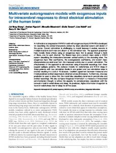
presented by the Gompertz and logistic functions, with negative estimates b and d, and the model II has presented positive estimates b and d, but with d < 1, which determines a curve without inflection point. The approximate estimated standard errors of the estimates a and c were, on average, two to three times greater in the model II, autoregressive, in comparison with models I and III, for logistic, Gompertz and Richards functions. This increasing is expected, because the variance of the parameters is underestimated when we do not consider autoregressive structures (Souza, 1998). Concerning to the estimated standard error of the estimate b, the same can be said for the logistic and Gompertz functions, but when the Richards function is adjusted, the estimated standard errors of b and d are not comparable among different models, since the curves showed different growth patterns. Durbin-Watson test for residuals (DW) in Table 4 was significant (p < 0.05), showing positive correlation among residuals of fitted models I and III. Model II, otherwise, was efficient in the sense of incorporate the correlations to the predicted values, resulting in independent errors for the group F; for the groups G and H the values are very close to the superior critical significance level. Model II was also efficient in controlling heteroscedasticity, which was present in the model I. Furthermore, all values of r, the estimative of the autocorrelation parameter in model II, were significant (p < 0.0001); thus one must preferably employ the autoregressive model in relation to models I and III. All the goodness of fit indicators, RMS, R2, AICc and BIC, showed that model II was the best one, followed by model III, and then by model I (Table 4). Mean square error in model II adjustment is, on average, four times smaller than the values in model I and 2.5 times smaller than in model III. F-statistic values in formula (10) were significant (p < 0.05) and were performed to verify the contribution of Richards autoregressive model, which has one additional parameter, in relation to logistic and Gompertz models; this shows a significant improvement in using this model. Gompertz and Richards show better indicators of goodness of fit than logistic (Table 4), i.e., smaller mean square errors (RMS) and Akaike’s information criteria (AICc). R2 values were similar in the adjustment of the three functions. On average, the logistic function presents lower estimates of asymptote, in relation to the other functions (Table 3). It seems to be a characteristic of logistics, underestimate mature weights and overestimate them in the early stages (Brown et al., 1976). This is probably due to the location of the point of inflection, fixed at one half of the asymptote. Figure 1 shows the fit of Richards autoregressive and mixed models to the data of the Holstein race cows. Second-order autoregressive models of logistic, Gompertz and Richards did not significantly improve the adjustment, in relation to first-order autoregressive model; residual mean squares were quite similar in both
Autoregressive and mixed models
500 400 300
yo
200
ye
100
z
0 0
10
20
30
40
50
60
x = age (months)
Figure 1 – First-order autoregressive (M II) and mixed (M III) Richards models fitted to 11 Holstein (H) cow weights. yo = observed values, ye = estimated values, z = deterministic part of the model.
35
Pinho et al.
Autoregressive and mixed models
Table 5 – Estimates of inflection (pi) and asymptotic deceleration (pda) points for logistic, Gompertz, and Richards functions fitted by models I (with independent errors), II (autoregressive) and III (mixed), and estimated standard errors (ep) for the abscissas of the points. Flemish (F), Guernsey × Gir (G), and Holstein (H) cow groups. Model
Function
MI
Logistic
Gompertz
Richards
M II
Logistic
Gompertz
M III
Logistic
Gompertz
Richards
Groups
xpi
ep(xpi)
xpda
ypda
ep(xpda)
F
18.0
244.1
0.57
46.4
443.4
1.67
G
14.7
208.2
0.37
37.2
378.2
1.07
H
15.9
249.6
0.43
40.6
453.5
1.20
F
12.1
191.5
0.50
46.3
441.1
2.06
G
9.6
158.7
0.32
35.1
365.6
1.19
H
10.6
194.9
0.39
40.1
449.0
1.55
F
12.4
194.1
0.61
46.4
441.5
-
G
9.9
161.6
0.41
35.3
366.6
-
H
10.7
195.8
0.42
40.1
449.1
-
F
24.3
284.9
2.40
51.9
517.4
6.10
G
19.0
239.6
1.28
40.7
435.3
3.31
H
17.6
262.2
1.03
40.8
476.4
3.00
F
16.5
214.1
1.85
50.6
493.1
6.88
G
12.6
174.8
0.98
37.9
402.6
3.60
H
11.0
194.5
0.82
37.7
448.0
3.41
F
17.7
242.2
0.55
45.4
440.0
1.63
G
14.7
207.6
0.36
36.8
377.1
1.05
H
15.7
248.2
0.44
40.0
450.8
1.23
F
12.1
191.4
0.47
46.3
440.9
1.94
G
9.7
159.1
0.19
35.3
366.4
0.73
H
10.6
194.3
0.28
39.8
447.6
1.12
F
12.2
192.7
0.52
46.6
442.3
-
G
9.7
159.5
0.22
35.2
365.9
-
10.6
194.0
0.25
39.4
445.2 xpda means
-
H Model
ypi
xpi means Logistic
Gompertz
Richards
Logistic
Gompertz
Richards
MI
16.19
10.78
10.99
41.39
40.49
40.59
M II
20.29
13.38
-
44.43
42.05
M III
16.03
10.79 xpi means
10.84
40.73
40.45 xpda means
Model1
40.37
Logistic
Gompertz
Richards
Logistic
Gompertz
Richards
MI
15.56
10.44
10.66
38.25
36.81
36.93
M II
17.31
11.27
0.15
38.14
36.27
18.80
M III
15.62
10.49
10.57
38.36
36.97
37.04
1
Values calculated with 11 animals.
rity at point of inflection’, was 0.372 in Richards models I and III, a similar value as the constant in Gompertz, 0.368, and smaller than 0.5 in the logistic function. In model II, however, the value is very early, the ratio ypi/a is only 0.080. This anticipation in the occurrence of the inflection point of functions with flexibility in its location is reported by Porter et al. (2010). The asymptotic deceleration points, pda, were nearly the same for the three functions and models I and III ( 41 months, three races in average). A small increasing in this value was found for logistic and Gompertz in model II autoregressive. Concerning the analysis with 11 animals one sees a discrepant value for Richards autoregressive model (18.8 months, three races in average); at this age, the estimated weight is 278.1 in average, with ratio ypda/a equal to 0.529, a substantially lower value in comparison with the constants 0.908 in logistic and 0.847
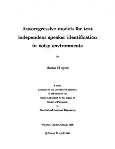
in Gompertz functions. The weight that was reached in this point is only 53 % of the asymptote, which can not be indicated as a stability point, despite the better fit of this function. As a comparison, a segmented regression (Portz et al., 2000) fitted to data of the 25 animals led to an intersection point of two straight lines, one horizontal and other sloping, of 37.4 months. Figure 2 compares the position of pda points in Richards autoregressive and mixed models, for the fit of the 11 animals' weights that had curves with inflection points. Almost all MPE20% values are negative, meaning that z-function overestimates the observed values in the final stage of growth (Table 6). This is more pronounced in model II in relation to models I and III, being the ratio M II / M III largest in logistics than in Gompertz. The situation is similar in the case of the adjustment to 11 animals, in addition that z-function is not so over-
Sci. Agric. v.71, n.1, p.30-37, January/February 2014
36
Pinho et al.
Autoregressive and mixed models
Group F
Logistic
Gompertz
Richards
RMSz
MPE20% MI
M II
M III
M II
M III
0.272
-12.888
0.540
2590.2
1132.7
G
-0.329
-14.519
-0.174
2876.4
1524.3
H
-1.433
-6.640
-1.193
2070.1
1798.9
F
-0.345
-8.948
-0.322
1752.9
1042.1
G
-1.095
-10.167 -3.758
-1.210
2059.8
-1.860
-1.794
1821.5
1739.5
F
-0.321
-
-0.406
-
1046.5
G
-1.060
-
-1.101
-
1462.7
H
-1.852
-
-1.587
-
1743.8
Values calculated with 11 animals. Function
Logistic
Gompertz
Richards
Group
RMSz
MPE20% MI
M II
M III
M II
H
F
G
H
10
20
30
40
50
60
70
x = age (months) M III F
1459.4
H
G
600 500 400 300 200 100 0 0
G
H
F
G
H
600
y = weight (kg)
Function
M II F
y = weight (kg)
Table 6 – Comparison criteria for z-function fitting of logistic, Gompertz, and Richards functions with models I (with independent errors), II (autoregressive), and III (mixed): mean prediction error for the latest 20 % observations (MPE20%) and residual mean square of z-function (RMSz). Flemish (F), Guernsey × Gir (G), and Holstein (H) cow groups.
500 400 300 200 100 0
M III
F
-0.480
-3.136
-0.482
744.7
628.2
G
-0.359
-8.671
-0.543
1801.5
1143.2
H
-0.935
-3.034
-1.019
1214.8
1082.6
F
-1.168
-2.468
-1.171
581.9
562.3
G
-1.230
-5.780
-1.415
1294.0
1084.3
H
-1.533
-1.031
-1.614
1040.7
1018.4
F
-1.144
-2.283
-1.731
536.3
570.7
G
-1.197
-3.101
-1.342
1067.9
1089.4
H
-1.507
0.604
-1.590
1051.2
1023.0
estimated in the autoregressive Richards model. Using this criterion, MPE20%, Richards function gives the best fit, in the final stages of growth, followed by Gompertz. The same conclusion may be attained when we used the RMSz criterion, that evaluates all the period of growth. Therefore, we can consider critical points determined by the autoregressive Richards model as well adjusted, and the relatively early values as a characteristic of the function, that is recognized as more flexible with respect to the location of the inflection point, and consequently of the asymptotic deceleration point.
0
10
20
30
40
50
60
70
x = age (months)
Figure 2 – Asymptotic deceleration points, pda, fitted to data of three groups of cows, Flemish (F), Guernsey × Gir (G) and Holstein (H), through autoregressive (M II, ypda/a = 0.529) and mixed (M III, ypda/a = 0.848) Richards models. 11 animals in each group.
In the determination of critical points in growth curves adjusted with models with a fixed and a random part, as the autoregressive and mixed models here considered, the deterministic function must be employed. The criteria proposed to verify the fit of the deterministic function, i.e., residual mean square for this function, and mean prediction error in the final observations, have allowed the comparison of the functions. This showed that Richards fits better than Gompertz, and this is better than the logistic. The values obtained to estimate the abscissa of the deceleration asymptotic point in logistic and Gompertz autoregressive model can be used as a stability point, but the value obtained with Richards autoregressive model was a very early stability point.
References Conclusions With growth data of Flemish, Holstein and Guernsey-gir cows, the first-order autoregressive model was efficient in fit the logistic, Gompertz and Richards functions, eliminating the residual autocorrelation. Mixed model, however, had a better fit in relation to fixed model with independent errors, but was not efficient in correcting the residual autocorrelation effect. Concerning the function, Richards fits better than logistic and Gompertz.
Sci. Agric. v.71, n.1, p.30-37, January/February 2014
Agudelo-Gómez, D.; Hurtado-Lugo, N.; Cerón-Muñoz, M.F. 2009. Growth curves and genetic parameters in Colombian buffaloes (Bubalus bubalis Artiodactyla, Bovidae). Revista Colombiana de Ciencias Pecuarias 22: 178-188. Bergamasco, A.F.; Aquino, L.H.de; Muniz, J.A. 2001. Non linear models fitting to growth data in females of the Holstein heifers. Ciência e Agrotecnologia 25: 235-241 (in Portuguese, with abstract in English). Bertalanffy, L. von. 1957. Quantitative laws for metabolism and growth. The Quarterly Review of Biology 32: 217-231.
37
Pinho et al.
Breusch, T.S.; Pagan, A.R. 1979. A simple test for heteroscedasticity and random coefficient variation. Econometrica 47: 12871294. Brody, S. 1945. Bioenergetics and Growth. Reinhold, New York, NY, USA. Brown, J.E.; Fitzhugh Jr, H.A.; Cartwright, T.C. 1976. A comparison of nonlinear models for describing weight-age relationships in cattle. Journal of Animal Science 42: 810-818. Calegario, N.; Calegario, C.L.L.; Maestri, R.; Daniels, R. 2005. Improving fitting quality of forest biometric models by applying the generalized nonlinear model theory. Scientia Florestalis 69: 38-50 (in Portuguese, with abstract in English). Craig, B.A.; Schinckel, A.P. 2001. Nonlinear mixed effects model for swine growth. The Professional Animal Scientist 17: 256260. Draper, N.R.; Smith, H. 1998. Applied Regression Analysis. 3ed. John Wiley, New York, NY, USA. 706p. Ersoy, I.E.; Mendes, M.; Aktan, S. 2006. Growth curve establishment for American Bronze turkeys. Archiv Tierzucht 49: 293-299. Fitzhugh Jr, H.A. 1976. Analysis of growth curves and strategies for altering their shape. Journal of Animal Science 42: 10361051. Gompertz, B. 1825. On the nature of the function expressive of the law of human mortality, and on a new method of determining the value of life contingencies. Philosophical Transactions of the Royal Society 182: 513-585. Mazzini, A.R.A; Muniz, J.A.; Silva, F.F.; Aquino, L.H. 2005. Growth curve for hereford males: heterocedasticity and autoregressives residuals. Ciência Rural 35: 422-427 (in Portuguese, with abstract in English). Mendes, P.N.; Muniz, J.A.; Silva, F.F.; Mazzini, A.R.A.; Silva, N.A.M. 2009. Analysis of the difasics growth curve of Hereford females by the Gompertz non-linear function. Ciência Animal Brasileira 10: 454-461 (in Portuguese, with abstract in English).
Autoregressive and mixed models
Mischan, M.M.; Pinho, S.Z.; Carvalho, L.R. 2011. Determination of a point sufficiently close to the asymptote in nonlinear growth functions. Scientia Agricola 68: 109-114. Narinc, D.; Karaman, E.; Firat, M.Z.; Aksoy, T. 2010. Comparison of non-linear growth models to describe the growth in Japanese Quail. Journal of Animal and Veterinary Advances 9: 19611966. Oehlert, G.W. 1992. A note on the delta method. The American Statistician 46: 27-29. Porter, T.; Kebreab, E.; Darmani Kuhi, H.; Lopez, S.; Strathe, A.B.; France, J. 2010. Flexible alternatives to the Gompertz equation for describing growth with age in turkey hens. Poultry Science 89: 371-378. Portz, L.; Dias, C.T.S.; Cyrino, J.E.P. 2000. A broken-line model to fit fish nutrition requirements. Scientia Agricola 57: 601-607. Richards, F.J. 1959. A flexible growth function for empirical use. Journal of Experimental Botany 10: 290-300. Schinckel, A.P.; Craig, B.A. 2002. Evaluation of alternative nonlinear mixed effects models of swine growth. The Professional Animal Scientist 18: 219-226. Souza, G.S. 1998. Introduction to Models of Linear and Nonlinear Regression = Introdução aos Modelos de Regressão Linear e Não Linear. Embrapa-SPI/Embrapa-SEA, Brasília, DF, Brasil. 489 p. Terra, M.F.; Muniz, J.A.; Savian, T.V. 2010. Fitting the logistic and Gompertz models to growth data of fruits of date palm-dwarf (Phoenix roebelenii O’BRIEN) = Ajuste dos modelos logístico e Gompertz aos dados de crescimento de frutos de tamareira-anã (Phoenix roebelenii O’BRIEN). Magistra 22: 01-07. Verhulst, P.-F. 1845. Mathematical researches into the law of population growth increase. Nouveaux Mémoires de l’Academie Royale des Sciences et Belles-Lettres de Bruxelles 18: 1-42.
Sci. Agric. v.71, n.1, p.30-37, January/February 2014