the electromagnetic field such that the total momentum of an isolated system, Pe+PT +PEM in the present example, is constant in time. A further subtlety is that ...
Cullwick’s Paradox: Charged Particle on the Axis of a Toroidal Magnet Kirk T. McDonald Joseph Henry Laboratories, Princeton University, Princeton, NJ 08544 (June 4, 2006)
1
Problem
In an induction linac [1] a toroidal solenoid magnet carries a time-dependent current I(t) such that the induced electric field can transfer energy from the magnet to charged particles that move along the axis of the toroid. Discuss the force and momentum balance in an idealized induction linac consisting of a single magnet whose form is a torus of major radius a and minor radius b � a, and a single electron of charge e that moves along the symmetry axis of the toroid. The current I is the total current crossing any major circle on the surface of the torus.
While actual induction linacs contain high-permeability ferrites inside the toroid, whose windings are made from shielded or unshielded conductors, it suffices here to consider a nonconducting toroid (without ferrites) whose currents are due to electric charges fixed on the rims of rotating disks. Neighboring disks have opposite charges and rotate in opposite senses so that the net electric charge (and the net mechanical angular momentum) of the toroid is zero. This configuration of a nonconducting toroid has no azimuthal current, in contrast to a single-layer helical winding on the toroid which includes, in effect, a single azimuthal current loop. You may assume that (unlike the case of an induction linac) the velocity v of the moving charge e of rest mass m is small compared to c, the speed of light, and that the time variation of the current in the toroid is slow enough that radiation and retarded effects can be ignored. Provide an analysis in the rest frame of the moving charge as well as in the lab frame, i.e., the rest frame of the toroid.
1
Cullwick [2, 3] has noted that this example is paradoxical because no force is exerted on the moving charge when the current is constant in the toroid, but the moving charge exerts a nonzero force on the toroid.
2
Solution
The force Fe on the electric charge e due to the toroid causes a time rate of change of the mechanical momentum Pe of the electron according to Fe =
dPe , dt
(1)
and likewise the force FT on the toroid changes the mechanical momentum PT of the latter according to dPT . (2) FT = dt The paradox (which dates back to Amp`ere) is that the magnetic interaction of a moving charge and a current (as well as the magnetic interaction of two moving charges) does not in general obey Newton’s third law, Fe �= −FT , so that the total mechanical momentum of the system, Pmech = Pe + PT , is not constant in time, in apparent violation of Newton’s first law for an isolated system. The resolution of such paradoxes is that electromechanical systems in general possess an additional momentum, PEM , associated with the interaction of the charges and currents with the electromagnetic field such that the total momentum of an isolated system, Pe +PT +PEM in the present example, is constant in time. A further subtlety is that the sum Pmech + PEM , while constant, may appear to have a nonzero value for an isolated system at rest. However, a “hidden” mechanical momentum Ph can be identified that restores the total momentum of a system at rest to zero.
2.1 2.1.1
Analysis in the Lab Frame The Electromagnetic Momentum
For systems in which effects of radiation and of retardation can be ignored, the electromagnetic momentum can be calculated in various equivalent ways [4] (in Gaussian units), �
PEM =
�A dVol = c
�
E×B dVol = 4πc
�
ΦJ dVol, c2
(3)
where � is the electric charge density, A is the magnetic vector potential (in the Coulomb gauge where ∇ · A = 0), E is the electric field, Φ is the electric (scalar) potential, and J is the electric current density. The first form is due to Faraday [5] and Maxwell [6], the second form is due to Poynting [7] and Abraham [8], and the third form was introduced by Furry [9]. To calculate the electromagnetic momentum using the first form of eq. (3), we need the vector potential AT of the toroid at the position of the charge e, but we do not need the 2
vector potential of the charge since the toroid is assumed to be electrically neutral. The vector potential of the toroid obeys ˆ ∇ × AT = BT = BT φ,
(4)
ˆ is a unit where the magnetic field is BT = 2I/ac inside the toroid and zero outside, and φ vector in the azimuthal direction in a cylindrical coordinate system (ρ, φ, z). The toroid is centered on the origin with the z-axis as its axis, as shown in the figure below (with radius b exaggerated for clarity).
Cullwick notes [3] that the relation (4) has the same form as Maxwell’s equation for the magnetic field due to a conducting wire that forms a (solid) torus of the same dimensions as ˆ the (hollow) toroidal magnet when the wire carries azimuthal current density J = J φ, ∇ × Bloop =
4π 4π ˆ J= J φ. c c
(5)
From the Biot-Savart law we know that the magnetic field along the axis of the current loop is, for b � a, 2π πb2J a2 ˆz . Bloop(0, 0, z) ≈ (6) c (z 2 + a2)3/2 Comparing eqs. (4) and (5), we see that on replacing 4πJ in eq. (6) by 2I/a we obtain the vector potential on the axis of the toroid when b � a, AT (0, 0, z) ≈
πb2I a ˆz . c (z 2 + a2)3/2
(7)
Hence, the electromagnetic momentum of the system when charge e is at position z on the axis of the toroid is PEM =
πb2 Ie eAT (0, 0, z) a ˆz , = c c2 (z 2 + a2 )3/2
which is independent of the velocity of the charge. 3
(8)
To calculate the electromagnetic momentum using the second form of eq. (3), we note that the electric field at the toroid due to charge e has magnitude Ee = e/(z 2 + a2 ) on average, and that the z-component of Ee ×√BT (which is the only one remaining after the integral over the toroid volume) is Ee BT a/ z 2 + a2. Hence,1 �
PEM =
e 2I a E e × BT 2πaπb2 a πb2Ie √ ˆz . ˆ dVol ≈ 2 z = 2 2 2 2 2 4πc z + a ac z + a 4πc c (z + a2)3/2
(9)
For completeness, we calculate the electromagnetic momentum using the third form of eq. (3). We must keep the first correction to the spatial dependence of the electric potential Φe of charge e over the toroid. Referring to the figure above, we see that r = � 2 R − 2bR cos(α + β) + b2 ≈ R[1 − Rb cos(α + β)], sin β = (a + b sin α)/r ≈ a/R, and √ R = z 2 + a2 . Only the z-component of the integral survives, so noting that Jz dVol → −Ib sin α dα, we find �
PEM
2.1.2
�
2π eI Φe J = dVol = − b sin α dα ˆz c2 c2 r 0 � � � b eIb 2π sin α dα 1 + (cos α cos β − sin α sin β) zˆ ≈ − 2 cR 0 R 2 a πb Ie ˆz . = 2 2 c (z + a2 )3/2
(10)
The Force on the Electric Charge
The force Fe on the electric charge is due to the electric field ET induced when the current in the toroid changes. This field is conveniently calculated as the time derivative of the vector potential (7). Thus, Fe = eET = −
˙ πb2 Ie e ∂AT a ˆz , =− 2 2 c ∂t c (z + a2 )3/2
(11)
where I˙ = dI/dt, independent of the velocity of the charge. This force is nonzero only when the current I in the toroid is changing. 2.1.3
The Force on the Toroid
The magnetic field Be at a distance r from the moving charge e is given by Be = e
ˆr v evρ ˆ × 2 = 3 φ, c r cr
(12)
where v is its velocity, and ρ is distance from the observation point to the z-axis. This magnetic field acts on the current I in the toroid to exert a force on the latter given by �
FT =
evI I dl × Be = 2 c c
1
�
dlρ
ρ ˆz r3
(13)
The “self momentum” of charge e associated with the cross product Ee × Be is, as usual, assumed to be part of the mechanical momentum of the charge.
4
Referring to the figure above, we see that dlρ = b cos α dα, ρ = a + b sin α ≈ a, � r = R2 − 2bR cos(α + β) + b2 ≈ R[1 − Rb cos(α + β)], cos β = (z − b cos α)/r ≈ z/R, and √ R = z 2 + a2 . Then, �
FT
evI � 2π a b ≈ b cos α dα 3 1 + 3 (cos α cos β − sin α sin β) 2 c 0 R R 2 ev ∂AT 3evIπb az zˆ = − = , 2 2 2 5/2 c (z + a ) c ∂z
�
ˆz (14)
recalling eq. (7). This force is nonzero whenever the velocity v of the charge and the current I in the toroid are nonzero. 2.1.4
Momentum Balance in the Lab Frame
The sum of the electromagnetic forces on the system is FT + Fe = −
e ∂AT ev ∂AT e dAT − =− , c ∂t c ∂z c dt
(15)
where d/dt is the convective derivative according to an observer on the charge e. The total force is nonzero when the charge is moving and/or the current in the toroid is changing, in apparent violation of Newton’s third law. Consistency with Newton’s laws is restored if we recall eq. (8) for the electromagnetic momentum of the system, so that we can write FT + Fe = −
∂PEM ∂PEM dPEM =− −v , dt ∂t ∂z
(16)
noting that the electromagnetic momentum varies both with the current in the toroid and with the position z of charge e. Then, using eqs. (1) and (2) we see that the total momentum of the system is constant in time, dPtotal dPT dPe dPEM + + = = 0. dt dt dt dt 2.1.5
(17)
“Hidden” Mechanical Momentum
While eq. (17) is a satisfactory representation of overall momentum balance, another aspect of momentum in this example remains paradoxical. Namely, that if the velocity of charge e is zero and toroid is at rest and contains a constant current, then the mechanical momenta Pe and PT appear to be zero, yet the electromagnetic momentum PEM of eq. (8) is nonzero. If the total momentum of an isolated system at rest is to be zero, in accordance with usual expectations, there must be an additional, “hidden” momentum in the system that is equal and opposite to the PEM . The question of whether the electromagnetic momentum (3) itself corresponds to a kind of “hidden” mechanical momentum was considered by Maxwell in secs. 552 and 590 of [10], who felt that the issue could not be settled at that time. Cullwick appears to have concluded that the electromagnetic momentum associated with currents actually is the mechanical 5
momentum of the moving charges that comprise the currents. See chap. 18 of [3]. However, this view does not ensure that the total momentum is zero for an isolated system at rest.2 Rather, we argue that if the charge e is brought sufficient slowly from “infinity” to rest near the toroid, then the force (14) is always negligible, and negligible work is done on the toroid during this process. The toroid remains at rest so long as the velocity of the charge e is negligible. The total energy of a charge e� of rest mass M that participates in the current I of the toroid remains Mc2 . When charge e is in the electric potential Φ = e/r of charge e, its electrical potential energy is e�Φ, so the effective mass Meff of charge e� is must be lower than M, such that ΔMeff = Meff − M = −e�Φ/c2 according to Einstein’s relation for the equivalence of mass and energy. Following initial discussion of this effect by Shockley [11] and by Coleman and Van Vleck [12], a useful expression for the “hidden” mechanical momentum Ph was given by Furry [9], Ph = −
�
ΦJ dVol. c2
(19)
who noted that for a single charge e�, J dVol ↔ e� v, so that the “hidden” mechanical momentum associated with ΔMeff is the dPh = −(e�Φ/c2 )v ↔ −(ΦJ/c2 ) dVol. Comparing with eq. (3) we see that (20) Ph = −PEM , (and not +PEM as argued by Cullwick [3]), so that the total momentum is indeed zero.3
2.2
Analysis in the Rest Frame of the Moving Charge
The transformation from the lab frame to the rest frame of charge e requires a boost by the small velocity v, and so we expect the forces to be the same in both frames. However, in the rest frame of the charge e that charge creates no magnetic field, so it appears that the force on the toroid is zero in this frame, and hence Galilean invariance may be violated. The resolution of this aspect of Cullwick’s paradox is to be found in the relativistic transformation of charge and current density, which form a 4-vector, (c�, J). We consider only the � case that the velocity v of charge e is small compared to the speed of light, so that γ = 1/ 1 − v 2/c2 ≈ 1. 2
Suppose that all the rest mass MT of the toroid is uniformly distributed on the rims of the disks of radius b that rotate with angular velocity ω = I/Q, where Q is the total charge on these disks. If we ignore the “hidden” mechanical momentum of eq. (19), the mechanical momentum of the toroid has only a z-component given by � � � 2π � V 2 + 2VT bω cos φ + b2 ω 2 dφ MT 2π PT = 1+ T (VT + bω cos φ) ˆz dφ γ(φ)MT Vz (φ) ˆ z ≈ 2π 2π 0 2c2 0 � � V 2 + 2b2 ω2 = MT VT 1 + T zˆ (18) 2c2 ˆ is the velocity of its center of mass. Then, if the toroid is at rest, VT = 0, its mechanical where VT = VT z momentum is also zero. 3 The present example, in which the mechanical momentum of conduction currents includes a “hidden” component, contrasts with others, [13, 14, 15] in which part or all of an isolated electromechanical system has tiny net velocity, such that the associated mechanical momentum is effectively “hidden”.
6
In the lab frame there is no charge density � associated in the toroid, but in the rest frame of charge e, whose lab velocity is v, the toroid has a nonzero charge density �� given by � � J · v J·v vJz ≈− 2 =− 2 , (21) �� = γ � − 2 c c c where the � indicates quantities measured in the rest frame of the charge. The lab-frame current consists of positive and negative charge densities that are equal and opposite but which have different velocities. On transforming to a moving frame, the positive and negative charge densities are no longer the same, and a net charge density (21) is observed. See sec. 86 of [16] for further discussion, including the example of a moving ring of current. Since the current density J resides on the surface of the toroid, the volume charge density (21) can be re-expressed as a surface charge density σ � given by σ� ≈
vI sin α, 2πac2
(22)
where α the angle shown in the figure above. The charge distribution (22) on the toroid is positive for radial distances ρ greater than a and negative for ρ < a, so that total charge on the toroid is zero in the rest frame (as well as in the lab frame). Charge e exerts an electrostatic force on the charge distribution (22) on the toroid, and, of course, charge e experiences an equal and opposite electrostatic force from the toroid (in addition to the force if the current is changing). For low-velocity transformations, the current density is unchanged since � = 0 in the lab frame,
(23) J� = γ J� − �v + J⊥ ≈ J. We now calculate the electromagnetic momentum P�EM , and the forces F�T on the toroid and F�e on the charge e in the rest frame of charge e. 2.2.1
The Electromagnetic Momentum
It is simplest to use the first form of eq. (3) to evaluate the electromagnetic momentum in the rest frame. The only vector potential in this frame is that due to the current J� ≈ J in the toroid. Hence, the rest frame vector potential A� obeys A� = A�T ≈ AT .
(24)
The rest-frame electromagnetic momentum is therefore,4 P�EM
�
=
��A� eAT dVol� ≈ = PEM , c c
(25)
the same as in the lab frame. This result illustrates how electromagnetic momentum that is tied to charges and currents does not transform like the space part of an energy-momentum 4-vector. See, for example, sec. 12.10 of [17] for additional comments. 4
We do not include the term σ � A�T /c in eq. (25) as this is suppressed a factor of c2 .
7
We can, however, relate the electromagnetic momentum to the charge/current-density 4-vector, (Φ, A). In the lab frame the electric potential ΦT of the toroid vanishes, so the transformation of the toroid’s lab-frame 4-vector (ΦT = 0, AT ) to the rest frame of charge e gives �
Φ�T 2.2.2
v · AT = γ ΦT − c
�
v ≈ − AT,z , c
�
A�T = γ AT,� − ΦT
�
v + AT,⊥ ≈ AT . c
(26)
The Force on the Toroid
The electric field E�e ≈ Ee = eˆr/r2 of charge e exerts a force F�T on the charge distribution σ� on the toroid in the charge’s rest frame given by5 F�T
�
= ≈
σ
�
� 2π 0
�
eˆr dArea� r2 � � ˆ − cos βˆ vI sin α e(sin β ρ z) b 1 + 2 cos(α + β) 2πab dα. 2πac2 R2 R
E�e
�
dArea =
σ�
(27)
A subtlety compared to the calculations in sec. 2.1 is that the factor cos β in the expression for ˆr in eq. (27) must be expanded to the next order of accuracy. Indeed, �
�
b z z z − b cos α 1 + cos(α + β) . ≈ ≈ cos β = r r R R
(28)
Thus, �
F�T
2.2.3
vIb � 2π b ˆ − z ˆz) 1 + 3 (cos α cos β − sin α sin β) ≈ 2 3 sin α e(a ρ cR 0 R 2 3evIπb ev ∂AT az ˆz = − = FT . ≈ 2 2 2 5/2 c (z + a ) c ∂z
�
dα (29)
The Force on the Electric Charge
The force F�e on the electric charge in its rest frame is due to the electric field E�T,ind induced when the vector potential of the toroid changes at the position of the charge e, and also due to the electric field E�T,σ� of the charge distribution (21) on the toroid. The vector potential A�T at the charge e is the same in the rest frame as in the lab frame, but in the rest frame A�T changes due to the velocity vT = −v of the toroid, as well as due to changes in the current I. Hence, the force due to the changing vector potential of the toroid is F�e,ind = eE�T,ind = −
e ∂A�T e e ∂AT ev ∂AT − (vT · ∇�T )A�T = − − , c ∂t c c ∂t c ∂z
(30)
noting that ∇�T = −∇�e (= −∇e ) since the former refers to the coordinates of the (center of the) toroid while the latter refers to the coordinates of the charge e. The electrostatic force 5
A briefer argument works backwards from the end of eq. (31).
8
on charge e is equal and opposite to the electrostatic force (27) on the toroid, �
�
−σ�ˆr ev ∂AT dArea� = −F�T = = −e∇�e Φ�T = −e∇e Φ�T (0, 0, z), 2 r c ∂z (31) where the last form refers to the electric potential (26) of the toroid in the rest frame of charge e. The total force on charge e in its rest frame is
F�e,σ � =
eE�T,σ� dArea� =
e
F�e = − 2.2.4
e ∂AT = Fe . c ∂t
(32)
Momentum Balance in the Rest Frame of Charge e
Once it is recognized that, in the rest frame of charge e, the moving toroid appears to have a nonzero surface charge distribution, we find that the forces on the charge and on the toroid are the same as in the lab frame. Also, the electromagnetic momentum is the same in both frames (which shows that PEM does not behave exactly like an ordinary momentum in all respects). Hence, the details of momentum balance are the same in both frames. The sum of the forces on the charge e and on the toroid in the rest frame is e dA�T dP� e ∂AT =− = − EM , (33) c ∂t c dt dt since the partial and total time derivatives of the vector potential at charge e are the same in the charge’s rest frame. Relating the forces to the corresponding time rates of change of momentum, we have dP�total dP�e dP�T dP�EM + + = = 0. (34) dt dt dt dt As expected, the total momentum is constant in the rest frame of the charge e. F�e + F�T = −
2.2.5
“Hidden” Mechanical Momentum in the Rest Frame of Charge e
According to the prescription of Furry [9], the “hidden” mechanical momentum in the rest frame of charge e can be calculated as6 �
Φ�e J� dVol� = −P�EM . (35) 2 c We have seen in eq. (23) that J� ≈ J. Similarly, the electric potential of charge e in its rest frame is that same as that in the lab frame when v � c, so that Φ�e ≈ Φe . Hence, P�h
=−
P�h ≈ Ph .
(36)
Thus, “hidden” mechanical momentum does not transform between moving frames like an ordinary mechanical momentum. The “hidden” momentum, as does the electromagnetic momentum, transforms like the charge-current 4-vector rather than like an energy-momentum 4-vector. Hence, both of these concepts must be treated with care in problems involving transformations between moving frames. See [18, 19] for additional commentary. 6
c.
We neglect the contribution from Φ�T J� /c2 in eq. (35) as this is suppressed by two additional powers of
9
2.3
Energy Considerations
2.3.1
Energy Flow in an Induction Linac
In the lab frame the charge e is accelerated by the electric field ET that exists when the current in the toroid is changing. The power P absorbed by the charge is ˙ 2 ev ∂ ev Iπb a . (37) P = Fe · v = evET (0, 0, z) = − AT (0, 0, z) = − 2 c ∂t c (z + a2)3/2 The flow of power from the toroid to the charge is described by the Poynting vector, or more precisely, by the interaction part of the Poynting vector, c c E T × Be + E e × BT . (38) Sint = 4π 4π It would be nice to have a plot of the field lines of the Poynting vector (38), which would show them emanating from the toroid and converging on the charge e. Lacking such a plot, we content ourselves with verification that the total Poynting flux across a small surface surrounding charge e, and also across the surface of the toroid, is equal to the power P of eq. (37). We first consider a small cylindrical surface of radius ρ and length 2l � ρ centered on the charge e. The electric field due to the toroid is essentially uniform over this surface, so ET ≈ ET (0, 0, z), and the magnetic field Be of charge e is given by eq. (12). Outside the toroid the magnetic field BT vanishes, so only the first term in eq. (38) contributes there. We can neglect the Poynting flux on the ends of the small cylinder since ρ � l. Hence, the inward Poynting flux over the surface of this cylinder is −
�
�
�
c c l evρ ˆ ˆ ET × Be · dArea ≈ − ET zˆ × 3 φ · 2πρ dz ρ 4π 4π −l cr � dz l evETρ2 l = evET √ 2 → evET = P, (39) ≈ 2 2 3/2 2 l + ρ2 −l (z + ρ )
Sint · dArea = −
in the limit that the radius ρ of the cylinder goes to zero. To evaluate the outward Poynting flux from the surface of the toroid we consider a toroidal surface just outside the actual toroid, so that the second term of eq. (38) can again be neglected. The electric field ET due to the changing current I˙ flows in loops of radius b just outside the toroid. From Faraday’s law, the magnitude of the induced electric field at the surface of the toroid is bI˙ bB˙ φ =− , (40) ET = − 2c ac recalling that Bφ = 2I/ac inside the toroid. The magnetic field of charge e at the toroid has magnitude Be = eva/c(z 2 + a2)3/2. The cross product ET × Be is directed along the outward normal to the surface of the toroid. Hence, the total outward Poynting flux from the toroid is � c c bI˙ eva ET Be Area = − Sint · dArea = 2πa 2πb 2 4π 4π ac c(z + a2)3/2 ˙ 2 ev Iπb a = − = P. (41) c (z 2 + a2 )3/2 10
2.3.2
Energy Balance in the Lab Frame
There are several forms of energy stored in the system, U = Ue + UT + Uint,
(42)
where the energy mv 2 (43) 2 of the moving charge includes its electromagnetic self energy. The energy UT of the toroid can be written (44) UT = UT,mech + UT,EM . Ue = γmc2 ≈ mc2 +
We suppose that all the rest mass MT of the toroid is uniformly distributed on the rims of the disks of radius b that rotate with angular velocity ω = I/Q, where Q is the total charge on these disks. Then, the mechanical energy of the toroid is � 2π
�
�
�
MT c2 2π dφ V 2 + 2VT bω cos φ + b2ω 2 ≈ UT,mech = γ(φ)MT c 1+ T dφ 2π 2π 0 2c2 0 MT (VT2 + b2ω 2) MT (VT2 + b2 I 2/Q2) = MT c2 + , (45) = MT c2 + 2 2 where VT = VT ˆz is the velocity of its center of mass. The electromagnetic energy stored in the toroid is � (2I/ac)2 BT2 ab2I 2 dVol ≈ 2πab2 = UT,EM = . (46) 8π 2c2 T 8π The electromagnetic interaction energy of the magnetic fields of the charge and toroid is �
Uint =
T
2
ab2Iev (2I/ac) eva BT · Be 2 2πab = , dVol ≈ 4π 4π c(a2 + z 2 )3/2 c(a2 + z 2 )3/2
where z = ze − zT is the distance between the charge and the center of the toroid. The time rate of change of the energy of the system is � � 2 2 ˙ ab ab2Iev ab2Iev˙ M b dU T ˙ ˙ ≈ mv v˙ + MT VT VT + + 2 II + + dt Q2 2c c(a2 + z 2 )3/2 c(a2 + z 2 )3/2 3ab2 Ievz(v − VT ) + . c(a2 + z 2 )5/2
(47)
(48)
For an induction linac, the toroid would be at rest in the laboratory (VT = 0 = V˙T ) and an external source would provide the power dU/dt that is transferred to the moving charge, as well as providing for the changes in the various other forms of energy of the system. We can also contemplate the idealized case of an isolated system with no external power source. Then, the total energy U is constant in time. The first two terms of eq. (48) can be written as Fe v + FT VT , and then using eqs. (11) and (21) we have that �
0 ≈
MT b2 ab2 + 2 Q2 2c
�
I˙ +
3ab2 ev 2z ab2ev˙ + , c(a2 + z 2 )3/2 c(a2 + z 2 )5/2
(49)
which relates the change in the current in the toroid to the change in the motion of the charge, such that energy is conserved. The derivatives I˙ and v˙ cannot both be negligible in an isolated system unless z is so large that the third term in eq. (49) is also negligible. 11
A
Appendix: Circuit Version of Cullwick’s Paradox
A variant on Cullwick’s paradox can be given in circuit form [20]. Consider a toroidal solenoid (1) and a simple LC circuit (2) in the form of a single-turn loop with a capacitor, as shown in the figure below. The LC circuit does not link the toroid. As usual in circuit analysis, we suppose that the frequency of the currents is low enough that they are spatially uniform in both the toroid and the LC circuit (and currents on the capacitor plates are neglected).
The EMF E 1 induced in the toroid by an oscillatory current I2 eiωt in the LC circuit is �
1d E1 = E1 (I2) · dl1 = − c dt 1
�
1 dI2 A1 (I2 ) · dl1 = − 2 c dt 1
� � 1
2
dl2 · dl1 ≡ −iωM12 I2, 2 r12
(50)
where the electrical field E = −∇V − ∂A/∂ct is entirely due to the vector potential A (if we ignore the small fringe field of the capacitor, as always done in circuit analysis), and the (retarded) vector potential is due only to the conduction current in the LC circuit [21] (see � also [22, 23, 24, 25, 26, 27, 28, 29, 30, 31, 32, 33, 34, 35]). That is, the integral 2 is restricted to the conductor of the LC circuit and does not include the “displacement current” in the gap between the capacitor plates.7 Then, the mutual inductance M12 is given by M12
1 � � dl2 · dl1 = 2 . 2 c 1 2 r12
(51)
If circuit 2 were a closed loop then M12 = 0, but in the present case M12 is nonzero. Similarly, the EMF E 2 induced in the LC circuit by current I1 eiωt in the toroid is given by �
1d E2 = E2 (I1) · dl2 = − c dt 2 �
�
1 dI1 A2 (I1 ) · dl2 = − 2 c dt 2
� � 2
1
dl1 · dl2 ≡ −iωM21 I1, 2 r21
(52)
where again the integral 2 is restricted to the conductor of the LC circuit. That is, the E2 does not include a contribution from the gap between the capacitor plates because there is no charge there for the electric field to act on (and E2 is unique only if the integral is restricted to the physical conductor).8 The mutual inductance M21 is given by M21
1 = 2 c
� � 2
1
dl1 · dl2 = M12, 2 r21
(53)
since r12 = r21 . 7
The unphysical result of [20] is based on the erroneous assumption that the “displacement current” ∂D/∂t is a source �of the vector potential (and of EMF). This leads to the misunderstanding that M12 = 0 when the integral 2 is taken to be over a closed loop so as to include the “displacement current”. 8 Another form of the circuit paradox would result from accepting that M12 is nonzero but erroneously supposing that the electric field in the gap of the capacitor contributes to the EMF induced in the LC circuit by the toroid. Typical analyses of LC circuits make this assumption with little error because the length of the gap between the capacitor plates is small compared to the circumference of the circuit. However, when the second loop is a toroid that is not linked by the LC circuit, including the electric field in the gap in the calculation of the EMF leads to the misunderstanding that M21 = 0.
12
A.1
Energy Conservation
For completeness, we perform an energy analysis of the coupled loops 1 and 2, supposing that they contain resistances R1 and R2 that dissipate energy. When the toroid is driven by an AC voltage source V eiωt , the loop equation for the toroid is V = R1 I1 + iωL1 I1 + iωM12I2,
(54)
where L1 is the self inductance of the toroid, and that for the LC circuit (which has no voltage source) is i 0 = R2 I1 + iωL2 I2 − I2 + iωM21I1. (55) ωC2 From eq. (55) we have that I2 = −
iω 2 M21C2 iω 2M21 C2 [ωR2 C2 − i(ω2 L2 C2 − 1)] = − I1 , I 1 ωR2C2 + i(ω 2 L2 C2 − 1) ω 2 R22 C22 + (ω 2 L2C2 − 1)2
(56)
and then eq. (54) tells us that
ω 3 M12M21 C2 [ωR2 C2 − i(ω2 L2 C2 − 1)] I1 . V = R1 + iωL1 + ω 2 R22 C22 + (ω 2 L2C2 − 1)2
(57)
The time-average power delivered by the voltage source is
1 ω 4M12 M21R2 C22 1 R1 + 2 2 2 |I1|2 , P = Re(V I1�) = 2 2 ω R2 C2 + (ω 2 L2 C2 − 1)2
(58)
while the power consumed in the toroid is 1 P1 = R1 |I1|2 , 2
(59)
and the power consumed in the LC circuit is 2 1 1 ω 4 M21 C22 2 2 |I1 | , P2 = R2 |I2| = R2 2 2 2 2 2 2 2 ω R2 C2 + (ω L2 C2 − 1)
(60)
recalling eq. (56). Thus, energy is conserved, P = P1 + P2 ,
(61)
since M21 = M12 according to eq. (53). Clearly, if the voltage source were connected to the LC circuit, rather than to the toroid, relation (61) would again hold.
13
A.2
Beyond the Approximations of Circuit Analysis
The preceding circuit analysis makes various approximations that are not strictly correct. The current in the circuits has been assumed to be spatially uniform, whereas there is a nonuniform surface current on both sides of the plates of the capacitor [34]. The effect of the electric fringe field of the capacitor has been neglected. The effect of the physical configuration of the voltage source on the electric and magnetic fields has been neglected. The effect of any measuring devices, used to probe the current in the circuits, has been neglected. The magnetic field outside the toroidal solenoid has been assumed to be zero in the quasistatic approximation, whereas it is actually nonzero [35]. Radiation has been neglected.9 The toroid, the capacitor, and the wire loop of the LC circuit are made of rather good conductors, at whose surface the tangential component of the electric field is negligible. That � is, E · dl is negligible for these good conductors, and is significantly nonzero only in the voltage source and in the load resistor. So, the forms (50) and (52) for the EMF s are not accurate (and the concept of mutual inductance is only approximate). To deal with all of these effects a more sophisticated analysis is required, of the sort made for antenna systems. There, systems with good conductors (with finite thicknesses) and possible, compact load capacitors, inductors and resistors are analyzed via an integral equation (due to Pocklington [37]) that incorporates the good-conductor boundary condition. These calculations are better performed numerically than analytically.10 Energy conservation is, of course, maintained throughout such analyses. When dealing with pairs of antennas, one transmitting and one receiving, as in the example of this Appendix, a reciprocity relation can be formulated (see, for example, [40]) between the drive voltages and driven currents when the roles of transmitter and receiver are reversed. This is a generalization of the condition M12 = M21 on the mutual inductances of circuit analyis. Thus, there exists a powerful formalism to go beyond the approximations of circuit analysis, although this formalism does not lend itself to simple analytic results, and we content ourselves with the circuit analysis given in the main part of this Appendix.
References [1] N.C. Cristofilos et al., High Current Linear Induction Accelerator for Electrons, Rev. Sci. Instr. 35, 585 (1964), http://puhep1.princeton.edu/~mcdonald/examples/accel/christofilos_rsi_35_88_64.pdf
[2] E.G. Cullwick, Nature 170, 425 (1952), http://puhep1.princeton.edu/~mcdonald/examples/EM/cullwick_nature_170_425_52.pdf 9 10
For discussion of a nominally simple circuit for which radiation cannot be ignored, see [36]. See, for example, [38] and [39] for analytic discussion of this approach.
14
[3] E.G. Cullwick, Electromagnetism and Relativity (Longmans, Green & Co., London, 1959), pp. 232-238, http://puhep1.princeton.edu/~mcdonald/examples/EM/cullwick_ER_59.pdf
[4] J.D. Jackson, Relation between Interaction terms in Electromagnetic Momentum � 3 d x E×B/4πc and Maxwell’s eA(x, t)/c, and Interaction terms of the Field Lagrangian � LEM = d3 x [E 2 − B 2]/8π and the Particle Interaction Lagrangian, Lint = eφ − ev · A/c (May 8, 2006), http://puhep1.princeton.edu/~mcdonald/examples/EM/jackson_050806.pdf [5] Part I, sec. IX of M. Faraday, Experimental Researches in Electricity (Dover Publications, New York, 2004; reprint of the 1839 edition). [6] Secs. 22-24 and 57 of J.C. Maxwell, A Dynamical Theory of the Electromagnetic Field, Phil. Trans. Roy. Soc. London 155, 459 (1865), http://puhep1.princeton.edu/~mcdonald/examples/EM/maxwell_ptrsl_155_459_65.pdf
[7] J.H. Poynting, On the Transfer of Energy in the Electromagnetic Field, Phil. Trans. Roy. Soc. London 175, 343 (1884), http://puhep1.princeton.edu/~mcdonald/examples/EM/poynting_ptrsl_175_343_84.pdf
[8] M. Abraham, Prinzipien der Dynamik des Elektrons, Ann. Phys. 10, 105 (1903), http://puhep1.princeton.edu/~mcdonald/examples/EM/abraham_ap_10_105_03.pdf
[9] W.H. Furry, Examples of Momentum Distributions in the Electromagnetic Field and in Matter, Am. J. Phys. 37, 621 (1969), http://puhep1.princeton.edu/~mcdonald/examples/EM/furry_ajp_37_621_69.pdf
[10] J.C. Maxwell, A Treatise on Electricity and Magnetism, 3rd ed. (Clarendon Press, Oxford, 1894; reprinted by Dover Publications, New York, 1954). The first edition appeared in 1873. [11] W. Shockley and R.P. James, “Try Simplest Cases” Discovery of “Hidden Momentum” Forces on Magnetic Currents, Phys. Rev. Lett. 18, 876 (1967), http://puhep1.princeton.edu/~mcdonald/examples/EM/shockley_prl_18_876_67.pdf
[12] S. Coleman and J.H. Van Vleck, Origin of “Hidden Momentum” Forces on Magnets, Phys. Rev. 171, 1370 (1968), http://puhep1.princeton.edu/~mcdonald/examples/EM/coleman_pr_171_1370_68.pdf
[13] K.T. McDonald, “Hidden” Momentum in a Coaxial Cable (Mar. 28, 2002), http://puhep1.princeton.edu/~mcdonald/examples/hidden.pdf
[14] K.T. McDonald, Momentum in a DC Circuit (May 26, 2006), http://puhep1.princeton.edu/~mcdonald/examples/loop.pdf
[15] K.T. McDonald, “Hidden” Momentum in a Sound Wave (Oct. 31, 2007), http://puhep1.princeton.edu/~mcdonald/examples/hidden_sound.pdf
15
[16] R. Becker, Electromagnetic Fields and Interactions (Dover Publications, New York, 1964). [17] J.D. Jackson, Classical Electrodynamics, 3rd ed. (Wiley, New York, 1999). [18] V. Hnizdo, Hidden momentum and the electromagnetic mass of a charge and current carrying body, Am. J. Phys. 65, 55 (1997), http://puhep1.princeton.edu/~mcdonald/examples/EM/hnizdo_ajp_65_55_97.pdf
[19] K.T. McDonald, On the Definition of “Hidden” Momentum (July 9, 2012), http://puhep1.princeton.edu/~mcdonald/examples/hiddendef.pdf
[20] Y. Liang, Q. Liang, and X. Liu, An Experimental Evidence of Energy Non-Conservation, http://puhep1.princeton.edu/~mcdonald/examples/EM/liang_1005.0078.pdf
[21] L. Lorenz, Ueber die Identit¨at der Schwingungen des Lichts mit den elektrischen Str¨omen, Ann. Phys. 207, 243 (1867), http://puhep1.princeton.edu/~mcdonald/examples/EM/lorenz_ap_207_243_67.pdf
On the Identity of the Vibration of Light with Electrical Currents, Phil. Mag. 34, 287 (1867), http://puhep1.princeton.edu/~mcdonald/examples/EM/lorenz_pm_34_287_67.pdf [22] S.J. Raff, Ampere’s Law and the Vector Potential, Am. J. Phys. 26, 454 (1958), http://puhep1.princeton.edu/~mcdonald/examples/EM/raff_ajp_26_454_58.pdf
[23] A.P. French and J.P. Tessman, Displacement Current and Magnetic Fields, Am. J. Phys. 31, 201 (1963), http://puhep1.princeton.edu/~mcdonald/examples/EM/french_ajp_31_201_63.pdf
[24] R.M. Whitmer, Calculation of Magnetics and Electric Fields from Displacement Currents, Am. J. Phys. 33, 481 (1965), http://puhep1.princeton.edu/~mcdonald/examples/EM/whitmer_ajp_33_481_65.pdf
[25] E.G. Cullwick, The Fundamentals of Electro-Magnetism, 3rd ed. (Cambridgue U. Press, 1966), chap. 3, sec. 14. [26] W.G.V. Rosser, Displacement current and Maxwell’s equations, Am. J. Phys. 43, 502 (1975), http://puhep1.princeton.edu/~mcdonald/examples/EM/rosser_ajp_43_502_75.pdf Does the displacement current in empty space produce a magnetic field?, Am. J. Phys. 44, 1221 (1976), http://puhep1.princeton.edu/~mcdonald/examples/EM/rosser_ajp_44_1221_76.pdf
[27] A. Shadowitz, The Electromagnetic Field (McGraw-Hill, 1977; Dover reprint, 1978), sec. 11-2. [28] W.G.V. Terry, The connection between the charged-particle current and the displacement current, Am. J. Phys. 50, 742 (1982), http://puhep1.princeton.edu/~mcdonald/examples/EM/terry_ajp_50_742_82.pdf
16
[29] W.G.V. Rosser, The displacement current, Am. J. Phys. 51, 1149 (1983), http://puhep1.princeton.edu/~mcdonald/examples/EM/rosser_ajp_51_1149_83.pdf
[30] T.A. Weber and D.J. Macomb, On the equivalence of the laws of Biot-Savart and Ampere, Am. J. Phys. 57, 57 (1989), http://puhep1.princeton.edu/~mcdonald/examples/EM/weber_ajp_57_57_89.pdf
[31] O.D. Jefimenko, Comment on “On the equivalence of the laws of Biot-Savart and Ampere”, Am. J. Phys. 58, 505 (1990), http://puhep1.princeton.edu/~mcdonald/examples/EM/jefimenko_ajp_58_505_90.pdf
[32] D.F. Bartlett, Conduction current and the magnetic field in a parallel plate capacitor, Am. J. Phys. 58, 1168 (1990), http://puhep1.princeton.edu/~mcdonald/examples/EM/bartlett_ajp_58_1168_90.pdf
[33] D.J. Griffiths and M.A. Heald, Time-dependent generalizations of the Biot-Savart and Coulomb laws, Am. J. Phys. 59, 111 (1991), http://puhep1.princeton.edu/~mcdonald/examples/EM/griffiths_ajp_59_111_91.pdf
[34] K.T. McDonald, Magnetic Field in a Time-Dependent Capacitor (Oct. 30, 2003), http://puhep1.princeton.edu/~mcdonald/examples/displacement.pdf
[35] K.T. McDonald, Electromagnetic Fields of a Small Helical Toroidal Antenna (Dec. 8, 2008), http://puhep1.princeton.edu/~mcdonald/examples/cwhta.pdf [36] K.T. McDonald, A Capacitor Paradox (July 10, 2002), http://puhep1.princeton.edu/~mcdonald/examples/twocaps.pdf
[37] H.C. Pocklington, Electrical Oscillations in Wires, Proc. Camb. Phil. Soc. 9, 324 (1897), http://puhep1.princeton.edu/~mcdonald/examples/EM/pocklington_camb_9_324_97.pdf
[38] K.T. McDonald, Voltage Across the Terminals of a Receiving Antenna (June 25, 2007), http://puhep1.princeton.edu/~mcdonald/examples/receiver.pdf
[39] K.T. McDonald, Currents in a Center-Fed Linear Dipole Antenna (June 27, 2007), http://puhep1.princeton.edu/~mcdonald/examples/transmitter.pdf
[40] K.T. McDonald, An Antenna Reciprocity Theorem (Apr. 3, 2010), http://puhep1.princeton.edu/~mcdonald/examples/reciprocity.pdf
17