Example. Robert G. Reynolds, Bin Peng. Department of Computer Science, Wayne State University,. Detroit, MI 48202. {reynolds, pebi}@cs.wayne.edu. Abstract ...
Cultural Algorithms: Computational Modeling Of How Cultures Learn To Solve Problems: An Engineering Example Robert G. Reynolds, Bin Peng Department of Computer Science, Wayne State University, Detroit, MI 48202 {reynolds, pebi}@cs.wayne.edu
Abstract. Our previous work on real-valued function optimization problems had shown that cultural learning emerged as the result of meta-level interaction or swarming of knowledge sources, “knowledge swarms” in the belief space. These meta-level swarms induced the swarming of individuals in the population space, “Cultural Swarms”. The interaction of these knowledge sources produced emergent phases of problem solving. In this paper we apply the approach to a real-world problem in engineering design. We observe the emergence of these same features in a completely different problem environment. We conclude by suggesting the emergent features are what give cultural systems their power to learn and adapt.
1 Introduction The Culture Algorithm was introduced by Reynolds as a vehicle for modeling social evolution and learning in agent-based societies [1, 2]. A Cultural Algorithm consists of an evolutionary population of agents whose experiences are integrated into a belief space consisting of various forms of symbolic knowledge. The Cultural Algorithm framework easily lends itself to supporting various types of learning activities including ensemble learning. The various knowledge sources in the belief space can be viewed as an ensemble of classifiers with the acceptance function collecting sample data using techniques such as bagging and boosting from the agent population. The influence function reflects the influence of the ensemble on the agent actions. Cultural Algorithms have been successfully applied in a number of diverse application areas [3]. In the process of doing this, five general types of knowledge have been gradually added to the cultural space that represent generic knowledge found in cultural systems. The knowledge sources include normative knowledge, spatial knowledge (topographic), temporal (historic), domain knowledge, and exemplar knowledge. Recently we have begun to look at the mechanisms by which the cultural knowledge works to solve problems posed to the social group. We were inspired to do this by the work of Kennedy and Eberhart on Particle Swarm Optimization [4]. In the process, certain phases of problem solving emerged from the cultural system in terms of how the knowledge sources were integrated together to solve a problem [5]. Specifically, a coarse-grained phase allowed the system to identify regions to explore in the continuous space, and that was followed by a fine-grained phase where a
different set of knowledge sources took the lead. A third phase, backtracking took place when the search process stagnated, again with a different suite of operators taking the lead. Since these phases continually emerged in both static and dynamic environments we investigated in more detail how they reflected a systematic interaction between the individuals in the population space and the knowledge sources in the belief space. What we observed was the emergence of swarms of individuals moving within the problem space as a result of the interaction of the cultural knowledge. We called these collections of individuals “Cultural Swarms”. We then looked to see how the knowledge sources interacted in the belief space, and identified the “swarming of knowledge” at the meta-level. That is, the statistical distribution of newly generated individuals in the search space by each knowledge source could be described in terms of their mean location and a bounding box that encompassed those individuals that were within one standard deviation from the mean. Changes in the shape and overlap of these bounding boxes demonstrated how the results of one knowledge source can be an attractor for others. This emergent phenomenon was called a “knowledge swarm”. Thus, this swarming of knowledge sources at the meta-level induced a swarming at the population level. From the meta-level perspective it was clear that the interaction of the knowledge sources emulated an algorithmic process similar to branch and bound [6]. Thus, an algorithmic process emerged from the meta-level swarming of cultural knowledge sources in this problem domain. The problem domain consisted of an arbitrary number of cones placed over real-valued two-dimensional space, with the goal of the population to explore the space and find the optimum [7]. While this domain was potentially a complicated one, it still had the makings of a toy problem. In this paper we use a real-world engineering problem, a problem to which particle swarm approaches have been applied previously [8]. The problem consists of optimizing the tension/ compression of a spring weight. Again, we can visualize the emergence of a branch and bound algorithmic-like process as the result of the interaction of knowledge sources.
2 Cultural Algorithms As a dual inheritance system, Cultural Algorithm has two basic components: the Population Space and the Belief Space. In each generation, individuals in the Population Space are first evaluated with a performance function obj(). An acceptance function accept() is then used to determine which individuals will be allowed to update the Belief Space. Experiences of those chosen individuals are then added to the contents of the Belief Space via function update(). Next, knowledge from the belief space is allowed to influence the selection of individuals for the next generation of the population through the influence() function. This supports the idea of dual inheritance in that the population and the belief space are updated each time step based upon feedback from each other. The CA repeats this process for each generation until the pre-specified termination condition is met. In this way, the population component and the belief space component interact with, and support each other in a manner analogous to the evolution of human culture. Fig. 1 describes such a framework and the basic pseudocode of Cultural Algorithm is given as follows: Begin t = 0;
initialize Bt, Pt repeat evaluate Pt update(Bt, accept(Pt)) generate(Pt, influence(Bt)) t = t + 1; select Pt from Pt- 1 until (termination condition achieved) End Here Pt represents the Population component at time t, and Bt for the Belief Space at time t. The algorithm begins by initializing both the Population and the Belief Space. Then it enters the evolution loop until the termination condition is satisfied. update() Belief Space accept() select()
influence()
Population Space
obj()
generate()
Fig. 1. Framework of the Cultural Algorithm
2.1 Knowledge Sources Five basic categories of cultural knowledge have been identified based upon the literature in Cognitive Science and Semiotics: Normative Knowledge, Situational Knowledge, Domain Knowledge, History Knowledge, and Topographical Knowledge. Normative Knowledge is a set of promising variable ranges that provide standards for individual behavior and guidelines within which individual adjustments can be made [9]. Normative Knowledge leads individuals to “jump into the good range” if they are not already there. Situational Knowledge provides a set of exemplary cases that are useful for the interpretation of specific individual experiences in specific contexts. Situational Knowledge leads individuals to “move toward the exemplars”. Topographical Knowledge was originally proposed to reason about region-based functional landscape patterns [10]. The functional landscape is initially divided into cells at a certain level of granularity according to spatial characteristics and each cell keeps track of the best individual found so far in its region. Cells can be recursively subdivided into sub-cells under certain circumstances. Topographical Knowledge guides individuals towards the best performing cells in the search space. Domain Knowledge uses knowledge about the problem domain to guide search. For example, in a functional landscape composed of cones, knowledge about cone shape and the related parameters will be useful in reasoning about them during the search process.
Historical or Temporal Knowledge monitors the search process and records important events in the search. These important events may be either a significant move in the search space or a detection of landscape change. Individuals guided by the History Knowledge can consult those recorded events for guidance in selecting a move direction. The five categories of knowledge that have been identified in CA systems were added at different times to achieve different problem-solving capabilities [9, 10, 5]. Reynolds has suggested that this set of knowledge sources is complete in that any cultural knowledge can be expressed as some combination of the five. When woven together, they show interesting collective behaviors regarding their different roles in the search process. These collective behaviors result in what we call “Knowledge Swarms”. These five knowledge sources are used here with only minor modifications from the Cones-World problem. This rather seamless transition was another interesting and rather unexpected event. It suggests to us that these five knowledge sources provide sufficient coverage to deal with broad classes of problems. 2.2 The Evolutionary Programming Population Component In this configuration of the Cultural Algorithm, Evolutionary Programming (EP) is chosen for the population model. An EP algorithm skeleton is given as follows: Begin Initialize a population of N candidate solutions Evaluate the population while ( not terminate condition) Copy parents to create N children Mutate each child Evaluate the children Stochastically select the best N individuals Discard the poorest N individuals end while End The advantage of EP approaches is that they focus on the phenotypes of an entire reproductive population, while cultural features are expressed frequently at the phenotypic level [9]. The model easily fits into the Cultural Algorithm through binding the influence function of CA and the variation operator V of EP seamlessly together. 2.3 Communication Protocol The acceptance function selects the individual experiences that will be used to update the belief space at each generation. Here, the acceptance function will take the experiences of the top individuals in the population and use that information to update all of the knowledge structures. But more generally, if we view the knowledge sources to be part of an ensemble of cultural learners, then the acceptance function can exploit many techniques such as “bagging” and “boosting” that relate to the sampling of individual experiences from the population.
Individuals are updated using the same framework as in [3]. The key here is that the knowledge sources communicate with each other through the update process. That is, if one knowledge source produces a new high performing individual, that individual can be used to potentially adjust each of the other knowledge sources. This allows other sources to exploit this new knowledge. The influence function determines how the knowledge sources can influence the population. In general, there are many ways of combining the influences of the knowledge ensemble. They can interact together in a heterogeneous fashion or a single homogenous activity can be performed. Here both are employed. The approach taken here is to allow all of the knowledge sources to act on the population at a given time step in a heterogeneous fashion but only one homogeneous knowledge source can influence a given individual at that time step. When an individual is to be modified, one knowledge source is selected to perform the modification at each generation. The selection process is done via roulette wheel selection where the area on the wheel taken by a knowledge source is a function of its past success in producing improvements in individual performances. Thus, as the population moves through the search landscape some knowledge sources may become more successful and others less successful.
3 The Test Engineering Problem A Tension/Compression Spring Weight Minimization problem from [8] is used to demonstrate the applicability of the Cultural Algorithm system on solving real world engineering problems. 3.1 Problem Description The problem consists of minimizing the weight of a tension/compression spring subject to constraints on minimum deflection, shear stress, surge frequency, limits on outside diameter and on design variables. The design variables are the mean coil diameter D, the wire diameter d and the number of active coils N. The problem is expressed as follows: Minimize f ( X ) = ( N + 2 ) Dd2
(655 35)
Subject to D3 N 0 71785d 4 4 D 2 dD 1 g2 (X) = + -1 12566( Dd 3 d 4 ) 5108d 2 g1 (X) = 1-
g3 (X) = 1 g4 (X) =
140.45d
0
D2N
D d -1 1.5
0
0 (2)
The variables take the following ranges: 0.05
d
2.0, 0.25
D
1.3, 2.0
N
15.0
(3)
3.2 Constraint Handling Most engineering problems are inherently constrained optimization problems. Individuals that do not satisfy all of the given constraints are called infeasible solutions. Infeasible solutions can come from the initial population, when individuals are randomly generated from the search space; or they can also from offspring generations.. It is possible that an offspring individual generated from a feasible parent can violate the given constraints. There are many different methods for handling infeasible solutions and the typical approaches are given in [11]. Here we use the Penalty Function Method as given below: if (individual satisfies all constrains) fitness = obj(individual) else fitness = IN_FEASIBLE_VALUE endif This method penalizes infeasible solutions by imposing penalties on individuals that violate problem constraints. Here, since this is a minimization problem the “infeasible value” is a large positive value. This approach was selected since it fits our metaphor for cultural learning in that it reflects the price that individuals pay for violating environmental constraints, where the performance function is the environment here. This method is also simple to implement and widely used, and checking for feasibility takes little computational time here.
4 Experiments and Results Analysis In all of the experiments conducted here, the EP population size is 200, and the maximum number of generation is set to 5000. A population size of 200 was selected so that each of the five knowledge sources would be represented initially at the same non-trivial density in the population. The search volume was approximately 20 so the initial density was 1 individual per .1 cubic units and each knowledge source was initially represented by 40 individuals. Since the search space spreads into three (or more) dimensions, we developed MATLAB viewers to visualize the search process and to investigate the activities within the search space. In the viewer, individuals from the population (or their statistical properties) are plotted using different symbols to indicate which knowledge source is controlling the individual changes at that time step. The symbols and their corresponding knowledge sources are given in table 1. The knowledge source controlling each individual in the population plots are given in column 1. The bounding box for each knowledge source is given identified by lines given in the bounding box column.
Table 1. Representation Scheme for the Knowledge Sources
Knowledge Types Normative Situational Domain History Topographical
Individual O circle diamond triangle pentagram dot
Bounding Box (3 point) (2 point) (2 point) - - - (2 point) (1 point)
4.1 Overviews of the Landscape and Search (Best Trace Plots) In the best trace plots, a contour map of the feasible region found by the best individuals produced over the first 10 generations is plotted in a two-dimensional style. In the plot, the search space is projected onto two of the three total dimensions and the best individual so-far is displayed as an ‘X’, thus it looks like the best is in a “two dimensional space”. For a search space with n dimensions, there are n*(n-1)/2 such kinds of projection. The fitness contour map is plotted as shaded areas where all points in the “two dimensional space” have the same value(s) as the current best individual on the other dimension(s). In this contour map, shading (darkness / lightness) is used to indicate the fitness of the points in the search space and the lighter ones have lower fitness and thus are better individuals since the problem is one of minimization. The infeasible solutions are represented by the darkest color level which forms the large background area for the enclosed feasible solutions. Notice that in Fig. 2, the feasible region for wire diameter d and N or D (in 1st and 2nd figures) converges early on, and it is the relationship between the mean coil diameter, D, and the number of active coils, N, that exhibit the most potential for exploration in future generations. Thus, while the problem is inherently 3-dimensional the system quickly reduces it to 2 dimensions. We will focus the rest of our discussion on these two dimensions.
Fig. 2. Best Trace Plot of Dimensions (d, D), (d, N), and (D, N) at Generation 10
4.2 Population Swarm Plots We now investigate the swarming activity that emerges in both the population and belief spaces. The population swarm plots show the population of individuals moving within the search space. Recall that each individual is shape coded to reflect the knowledge source that has influences it in that generation. The location of the best individual so far is identified by an ‘X’. Since the results of d and N, and d and D are similar we discuss only d and D. We will focus on D and N as well.
Fig. 3. Population Swarm Plot of dimension (d, D) at Generation 1
Fig. 4. Population Swarm Plot of dimension (d, D) at Generation 3
Fig. 5. Population Swarm Plot of dimension (d, D) at Generation 10
Population Swarm in Dimensions d and D. Fig. 3 shows the initial generation of individuals in terms of dimensions d and D. Notice that the topographic influenced individuals quickly draw the individuals controlled by situational knowledge to the region, close to 0 for d. By generation 10 (Fig. 5) most of the individuals are swarming around that area, but topographic knowledge is still generating individuals throughout the space as a background process. Population Swarm in Dimensions D and N. Again topographic knowledge produces a result near the optimum during the coarse-grained search phase as shown in Fig. 6. This attracts the situational, domain, and history knowledge sources in the fine-grained phase. In Fig. 7 we see that the optimum area is now surrounded by several individuals controlled by situational knowledge who are exploiting the region. Individuals controlled by domain and history knowledge are still not present on the scene. In Fig. 8 individuals controlled by domain knowledge and history knowledge are now in the optimal area as well. These individuals are exploiting the area at a fine-grained level along with individuals controlled by situational knowledge. Normative knowledge still generates individuals in the surrounding region while topographic knowledge still generates individuals throughout the space as a background search, which if successful could trigger a backtracking process.
Fig. 6. Population Swarm Plot of dimension (D, N) at Generation 1
Fig. 7. Population Swarm Plot of dimension (D, N) at Generation 3
Fig. 8. Population Swarm Plot of dimension (D, N) at Generation 10
4.3 Meta-Level Knowledge Plots For each generation the mean location of those individuals guided by the same knowledge type is plotted as one point. A bounding box (see Table 1 for line styles for each knowledge type) around the mean represents the standard deviation of each mean produced during that generation for the mutation process. Thus, the smaller the bounding box the more focused is the generation of individuals. The overlap of the bounding boxes represents regions that are being mutually exploited by the knowledge sources. The location of the best individual of that generation is identified by an ‘X’. Knowledge Means and Standard Deviations in Dimensions d and D. The bounding boxes represent the focus of the generation process by each knowledge source. Notice that initially in Fig. 9 that the bounding boxes associated with the topographic and normative knowledge sources cover most of the space. This is viewed as the branching phase of the algorithmic process. Notice that by generation 8 (Fig. 10), the bounding boxes for the fine-grained search process have separated from those for the coarse-grained phase and have surrounded the optimal value for this pair of dimensions. These bounding boxes are effectively channeling new individuals into this area. This process is the same for dimensions d and N. From an algorithmic point of view, the coarse-grained operators produce new search branches within the space, and then the fine-tuning operators place bounds on selected regions for additional local search.
Fig. 9. Knowledge Swarm Plot of dimension (d, D) at Generation 1
Fig. 10. Knowledge Swarm Plot of dimension (d, D) at Generation 8
Knowledge Means and Standard Deviations in Dimensions D and N. The algorithmic process is even easier to observe when we look at Dimensions D and N, since they do not become fixed early on like dimension d. Figures 11 through 13 give the meta-level bounding boxes that generate individuals in the population from generations 1, 8, and 10 respectively. By generation 10 the optimum has been found. Notice that the topographic and normative knowledge sources guide the branching process initially. Their bounding boxes encompass most of the problem space in this dimension in Fig. 11. It is interesting to note that the orientation of these boxes is north to south reflecting the functional gradient that we observed first in Fig. 2. The knowledge sources are effectively channeling individuals along the gradient. By generation 8, the bounding boxes of the fine-tuning operators have begun to overlap in particular area of the feasible region and have begun to bound the search. By generation 10, the bounding box for each knowledge source overlaps around the optimal value for this pair of dimensions, thus channeling new individuals into that area primarily.
Fig. 11. Knowledge Swarm Plot of dimension (D, N) at Generation 1
Fig. 12. Knowledge Swarm Plot of dimension (D, N) at Generation 8
Fig. 13. Knowledge Swarm Plot of dimension (D, N) at Generation 10
5 Conclusions In this paper we have investigated how the knowledge sources associated with cultural knowledge control the search process of individuals in terms of an engineering optimization problem. The results suggest that the meta-level interaction of the knowledge sources produce a shift in their generative regions to reflect a basic branch and bound process in terms of finding the solution. Particular operators (normative and topographic) branch the search into new regions, and other operators
(situational, domain, and historic) work to focus the search within the expanded space. The system was given no feasible solution points to start with but the swarming of the knowledge sources at the belief level engendered by the problem constraints produced swarming at the population level and led to a quick convergence. Thus, the interaction of the knowledge source produced a synchronization of the generation boxes so as to allow the system to mimic a branch and bound process, branching first to various potential solutions in the coarse-grained process, and then bounding the solution region in the fine-grained process. The system therefore learned to combine the generative processes associated with the various knowledge sources in order to branch out to find feasible solutions, and then bound the solutions in the fine-tuning phase. Thus the interaction of the knowledge sources induced the generation of swarms of individuals at the population level reflects a branch and bound like algorithmic process. We call this effect the “knowledge induced algorithmic process”. In future work we will investigate the properties of the knowledge sources that are required to learn and mimic various algorithmic processes.
References 1. Reynolds, G. R. 1979. An Adaptive Computer Model of the Evolution of Agriculture for Hunter-Gatherers in the Valley of Oaxaca Mexico. Ph.D. Dissertation, Department of Computer Science, University Of Michigan. 2. Reynolds, G. R. 1994. An Introduction to Cultural Algorithms. In Proceedings of the 3rd Annual Conference on Evolutionary Programming, 131-139: World Scientific Publishing. 3. Rychtyckyj, N.; Ostrowski, D.; Schleis, G.; and Reynolds, G. R. 2003. Using Cultural Algorithms in Industry, in Proceedings of IEEE Swarm Intelligence Symposium, Indianapolis, Indiana. IEEE Press. 4. Kennedy, J. and Eberhart, R. C. 1995. Particle Swarm Optimization. In Proceeding of the IEEE International Conference on Neural Networks, 12-13, Perth, Australia, IEEE Service Center. 5. Reynolds, G. R.; and Saleem, S. 2003. The Impact of Environmental Dynamics on Cultural Emergence. Festschrift, in Honor of John Holland, 1-10, Oxford University Press. 6. Peng, B.; Reynolds, G. R.; and Brewster, J. J. 2003. Cultural Swarms. In Proceeding of IEEE 2003 Congress on Evolutionary Computation. Canberra, Australia.: IEEE Press. Forthcoming. 7. Morrison, R. and De Jong, K. (1999) “A Test Problem Generator for Non-Stationary Environments, ” in Proceedings of Congress on Evolutionary Computation, pp 2047-2053, IEEE Press, 1999. 8. Hu, X.; Eberhart, C. R.; and Shi, Y. 2003. Engineering Optimization with Particle Swarm. In Proceedings of the 2003 IEEE Swarm Intelligence Symposium, 53-57. Indianapolis, Indi.: IEEE Press. 9. Chung, C.; and Reynolds, G. R. 1998. CAEP: An Evolution-based Tool for Real-Valued Function Optimization using Cultural Algorithms. International Journal on Artificial Intelligence Tools 7(3): 239-291. 10. Jin, X.; and Reynolds, G. R. 1999. Using Knowledge-Based Evolutionary Computation to Solve Nonlinear Constraint Optimization Problems: a Cultural Algorithm Approach. In Proceeding of the 1999 Congress on Evolutionary Computation, 1672-1678. Washington DC, IEEE Press 11. Michalewicz, Z. 1996. Genetic Algorithm + Data Structures = Evolution Program. 3rd. Berlin; New York: Springer-Verlag.