Assuming no default on the government debt, using (1.1), the condition limtâo e-rtbt Ï 0, and allowing for discrete jumps in government debt, yields the ...
Currency Crises and Fiscal Sustainability Craig Burnside∗, Martin Eichenbaum†and Sergio Rebelo‡ Revised July 2003
This chapter discusses the relation between Þscal sustainability and the sustainability of a Þxed exchange rate regime. At the most general level, Þscal sustainability simply corresponds to the notion that a government’s intertemporal budget constraint holds without explicit default on its debt. This requires that the initial real value of a government’s debt be equal to the real present value of its future primary surpluses plus the present value of inßationrelated revenues (e.g. seigniorage). In contrast, sustainability of a Þxed exchange rate regime requires that the government not raise any inßation-related revenues.1 So under such a regime, Þscal sustainability reduces to the condition that the real value of a government’s initial debt must equal the real present value of its primary Þscal surpluses. The classic example of a Þxed exchange rate regime that is not sustainable is analyzed in the seminal papers of Krugman (1979) and Flood and Garber (1984). These authors consider a situation in which a government is running persistent primary deÞcits. A key implicit assumption of their analyses is that future primary surpluses will not be large enough to balance the government’s intertemporal budget constraint. Since it is unfeasible to indefinitely borrow and repay the resources needed to cover the ongoing deÞcits, the government will eventually have to print money to raise seigniorage revenues. This means that the Þxed exchange rate regime is not sustainable. As we will see below, the precise timing of the Þxed exchange rate collapse depends on various assumptions about government behavior and the demand for domestic money. But collapse it will. Precise timing aside, in this scenario an analyst would observe large ongoing deÞcits and rising debt levels prior to the collapse of the Þxed exchange rate regime. ∗
University of Virginia Northwestern University, NBER and Federal Reserve of Chicago. ‡ Northwestern University and NBER. 1 Here we abstract from growth in the demand for domestic money and foreign inßation. †
One might be tempted to conclude that large primary deÞcits are a necessary symptom of Þscal nonsustainability under a Þxed exchange rate regime. But that is not the case. Unless the assumptions of the Krugman-Flood-Garber analyses hold, it is very difficult to assess whether a given country is on a Þscally sustainable path using historical data on standard macroeconomic aggregates like deÞcits. Deciding whether a Þxed exchange rate regime is sustainable necessarily involves forecasting the future values of government purchases, transfers and tax revenues. This is particularly difficult in a world where governments incur large contingent liabilities. Such liabilities often arise because governments are committed to bailing out large sectors of the economy (e.g. banks and other large Þnancial institutions) should they fail. A government which was running substantial Þscal surpluses may switch to a Þscally nonsustainable path, once large contingent liabilities are triggered. This happens when the government does not have a credible way of raising future primary surpluses to pay for the activated liabilities. Under these circumstances, activated contingent liabilities translate into prospective deÞcits which the government must fund via inßation-related revenues. It follows that the Þxed exchange rate regime is no longer sustainable. Again, the precise time at which the collapse depends on various assumptions. But as in the Krugman-Flood-Garber case the collapse is inevitable. Below we display examples, motivated by the recent East Asian currency crises, in which the Þxed exchange rate regime collapses before the government begins to pay the activated liabilities, incur primary deÞcits or print money. In such a situation primary deÞcits are obviously a very poor indicator of Þscal nonsustainability. Instead the analyst must carefully assess the nature of a government’s contingent liabilities, the probability that those liabilities will be activated and the extent to which the government is willing to raise revenues not related to inßation to pay for its prospective expenditures. In practice such an assessment will involve detailed institutional information about the country in question. Statistical analysis of standard macroeconomic data–no matter how well informed by economic theory–will not suffice. The remainder of this chapter is organized as follows. Section 2 displays a simple version of the government budget constraint. In chapter XX we will discuss a more realistic version of the budget constraint that will be useful for organizing data and analyzing particular episodes. Here the crucial issue will be whether the government needs to raise resources via inßation-related revenues or not. Section 3 considers the classic Krugman-Flood-Garber
2
experiment. In Section 4 we turn to the case of currency crises triggered by prospective deÞcits. In addition we argue on empirical grounds that this case provides a good description of the origins of the East Asian currency crises. Section 5 brießy reviews the shortcomings of our analysis and serves as an introduction to chapter XX.
1. The Government’s Intertemporal Budget Constraint In this section we develop a simpliÞed version of the government’s intertemporal budget constraint. The key simpliÞcation is that the only inßation-related source of revenue available to the government is printing money. In chapter 3 we discuss additional sources of inßation-related revenue: deßating the real value of outstanding nonindexed nominal debt and reducing the real value of government expenditures by an implicit Þscal reform. By the latter we mean that the government can deßate the real value of its outlays that are Þxed, at least temporarily, in nominal terms (e.g. civil servant wages or social security payments). To proceed we assume that there is a single good whose domestic currency price is Pt . The foreign currency price of this good is Pt∗ and purchasing power parity (PPP) holds: Pt = Pt∗ St . Here St is the exchange rate expressed in units of local currency per unit of foreign currency (so a depreciation means a rise in St ). For simplicity we assume that Pt∗ = 1 so that Pt = St . The government can borrow and lend in international capital markets at a constant real interest rate r. It also has assets in the form of foreign reserves which earn the real interest rate rt . We denote the dollar value of the government’s debt net of foreign reserves by bt . Net government debt evolves according to: bú t = rbt − (τ t − gt − vt ) − Mú t /St .
(1.1)
The variable gt represents real government spending, vt represents real transfers and τ t real tax revenues. The term τ t − gt − vt represents the real government surplus, while Mt
denotes the level of the money supply. We use the notation xú to represent the derivative of x with respect to time, dx/dt. Equation (1.1) assumes that the government’s real debt and the supply of money evolve smoothly over time.2 In currency crisis models there are typically points in time at which M 2
Technically (1.1) applies when b and M are differentiable functions of time.
3
and b change discretely (one such point in time is the instance at which the exchange rate regime is abandoned). We denote the set of such points in time by I. At these points the change in government debt is given by: ∆bt = −∆(Mt /St ).
(1.2)
Assuming no default on the government debt, using (1.1), the condition limt→∞ e−rt bt = 0, and allowing for discrete jumps in government debt, yields the government’s intertemporal budget constraint: ! ∞ ! −rt b0 = (τ t − gt − vt )e dt + 0
∞
(Mú t /St )e−rt dt +
0
"
∆(Mt /St )e−rt .
(1.3)
t∈I
According to (1.3) the initial level of the government debt must be equal the present #∞ value of future surpluses ( 0 (τ t − gt − vt )e−rt dt) plus the present value of seigniorage #∞ $ ( (Mú t /St )e−rt dt + ∆(Mt /St )e−rt ). We say that a set of monetary and Þscal poli0
t∈I
cies is Þscally sustainable as long as (1.3) holds.
Fiscal sustainability is much more stringent in an economy operating under a Þxed exchange rate regime. Abstracting from foreign inßation the price level must be constant in a Þxed exchange rate regime, because otherwise PPP would not hold. Abstracting from growth in the demand for real balances (due to growth in output or consumption) this last condition requires that the money supply be constant, so that seigniorage revenues are zero. It follows that (1.3) reduces to: b0 =
!
0
∞
(τ t − gt − vt )e−rt dt.
(1.4)
The key point here is that sustainability of a Þxed exchange rate regime requires that the government balance its intertemporal budget constraint without resorting to inßation-based revenues. The forward looking nature of (1.4) makes clear why it is so difficult to determine from real time data whether a country is on a Þscally sustainable path. There is no way to evaluate Þscal sustainability without forecasting the future paths of expenditures and taxes. For example a country could be running a sustained deÞcit for a period of time yet (1.4) could still hold because the government will credibly run future surpluses that will offset the deÞcits. In contrast, a country could be running a surplus but have future deÞcits that are so large that (1.4) does not hold. This last possibility is more than a theoretical curiosity. Table 1 presents data on the Þscal surpluses for the United States and several Asian countries. Notice that the countries 4
involved in the Asian currency crises of 1997 (Indonesia, Korea, Malaysia, Philippines and Thailand) were running either surpluses or modest deÞcits. At the same time the U.S., which did not suffer large adverse movements in its exchange rate, was running a Þscal deÞcit. We will return to this example later when we discuss the importance of contingent liabilities and their impact on government budget constraints.
2. Fiscal Sustainability and Speculative Attacks When sustainability condition (1.4) does not hold it is inevitable that a Þxed exchange rate regime will be abandoned. The only questions are: when and what will the aftermath look like? The answers to these questions depends on three elements: (i) the nature of money demand; (ii) the rule for abandoning Þxed exchange rates; and (iii) the post-crisis monetary policy. We will now add these elements to our analysis and discuss two experiments. In the Þrst case there is an immediate increase in government transfers which induces the government to begin running a deÞcit. In the second case agents Þnd out that there will be an increase in future government transfers, say because contingent liabilities to a failing banking system have been activated. This will induces prospective, but not current, deÞcits. Money Demand We adopt a standard speciÞcation for the demand for domestic money, due to Cagan (1956): Mt = θY Pt e−ηRt ,
(2.1)
where θ is a positive constant. According to (2.1), the demand for domestic money depends positively on Y, the domestic real income of the economy, and negatively on the opportunity cost of holding money, the nominal interest rate, Rt . The parameter η represents the semielasticity of money demand with respect to the interest rate. For the sake of simplicity we assume that domestic real output is constant over time. In the absence of uncertainty the nominal interest rate is equal to the real rate of interest (rt ) plus the rate of inßation, π t = Pú t /Pt : Rt = rt + π t . Combining (2.1) and (2.2) we obtain a differential equation in Pt : log(Mt ) = log(θY ) + log(Pt ) − η(r + Pút /Pt ), 5
(2.2)
The solution to this equation is: 1 ln Pt = ηr − ln(θY ) + η
!
∞
e−(s−t)/η ln(Ms )ds.
(2.3)
t
Consistent with classic results in Sargent and Wallace (1973), equation (2.3) implies that the current price level is an increasing function of current and future money supplies. To see the intuition behind this result suppose that at time t the economy is under a ßoating exchange rate regime. Higher growth rates of money in the future translate into higher rates of inßation and a higher nominal interest rate. This in turn lowers the demand for real balances at time t. Under ßoating exchange rates Mt is exogenously determined by the central bank. So the only way for real balances to fall in equilibrium is for the price level to rise. Equation (2.3) also holds while the exchange rate is Þxed. Suppose Þrst that the Þxed exchange rate regime is sustainable. Then inßation is zero and Pt = S. The money supply, which is endogenous, must equal the quantity demanded given S: M = SθY exp(−ηr).
(2.4)
When the value of M is constant equation (2.3) reduces to: ln Pt = ηr − ln(θY ) + ln M
(2.5)
So if the level of the money supply is given by (2.4) then Pt = S. If the government tried to print more money than the level M given by (2.4), private agents would simply trade it in at the Þxed exchange rate for foreign reserves or government debt. Thus, as long as the country is in a Þxed exchange rate regime, the government cannot generate seigniorage revenues.3 The interpretation of (2.3) is more complicated when the exchange rate is Þxed at time t but agents know that at some future date t∗ the economy will let the exchange rate ßoat. After t∗ the path of the money supply is determined by the central bank, so the intuition for (2.3) is as described above. Before t∗ the money supply is endogenously determined by the behavior of private agents. To understand the role played by equation (2.3) before t∗ we must discuss the determinants of t∗ . We now turn to this task. 3
If there were growth in P ∗ or in Y , the government would collect some seignorage revenue in a Þxed exchange rate regime.
6
Rule for Abandoning Fixed Exchange Rates It is standard in the literature to assume that the government follows a threshold rule for abandoning the Þxed exchange rate regime: the Þxed exchange rate regime is abandoned in the Þrst period, t∗ , in which the government’s debt reaches some Þnite upper bound, ¯b. This rule turns out to be equivalent to another rule that we will use in our analysis: the Þxed exchange rate is abandoned when the amount of domestic money sold by private agents in exchange for foreign reserves exceeds some percentage of the initial money supply, i.e. when the money demand falls to e−χ M, for some χ > 0. To see why the two rules are equivalent, it is important to recognize that in any equilibrium where the Þxed exchange rate regime is abandoned, the inßation rate rises discretely at the time this occurs. Agents, anticipating this, will discretely reduce their domestic money balances an instant before the exchange rate regime is abandoned. Under the Þxed exchange rate regime they go to the government and exchange domestic money for dollars at rate S. This reduces the government’s reserves, thus raising its net debt. So the rise in debt that sets off the government’s threshold rule and the fall in money demand occur simultaneously. In addition to being a good description of what happens in actual crises, the threshold rule can be interpreted as a short-run borrowing constraint on the government: it limits the amount of reserves that the government can borrow to defend the Þxed exchange rate.4 Rebelo and Végh (2001) discuss the circumstances in which it is optimal for a social planner to follow a threshold rule.5 While they use a general equilibrium model, their framework is similar in spirit to the model used here. Post-crisis Monetary Policy Finally, we adopt the following speciÞcation of post-crisis monetary policy: in period T the government engineers a one time increase in the money supply relative to its pre-crisis level, i.e. MT = eγ M. Thereafter the money supply grows at the rate µ. This formulation for post-crisis money supply decouples the time of the speculative attack (which will be computed later) from the time at which the government 4
Drazen and Helpman (1987), as well as others, have proposed a different rule for the government’s behavior: Þx future monetary policy and allow the central bank to borrow as much as possible provided the present value budget constraint of the government is not violated. This rule ends up being equivalent to a threshold rule. See Wijnbergen (1991) and Burnside, Eichenbaum and Rebelo (2001) for a discussion. 5 Rebelo and Végh (2001) show that this rule for abandoning the peg is optimal when: (i) the Þscal shock that makes the Þxed exchange rate regime unsustainable is of moderate size; and either (ii) there are signiÞcant real social costs associated with a devaluation, such as loss of output or Þrm bankruptcy; or (iii) while the exchange rate is Þxed a Þscal reform may arrive according to a Poisson process that restores the sustainability of the Þxed exchange rate regime.
7
starts to print money. It also nests as a special case the speciÞcation used by Krugman (1979) and Flood and Garber (1984) according to which money starts growing at a constant rate µ as soon as Þxed exchange rate are abandoned. Finally, this speciÞcation is simple enough so that we can provide intuition about the timing of the speculative attack. As we will see below, in general, given the threshold rule and our assumptions about monetary policy, the Þxed exchange rate regime will be abandoned prior to time T . As we will establish, the Þxed exchange rate regime is abandoned when the money supply falls by χ percent, so the post-crisis behavior of the money supply can be summarized as follows: % e−χ M, for t∗ ≤ t < T Mt = (2.6) for t ≥ T . eγ+µ(t−T ) M, With these elements in place we can now discuss the timing of the speculative attack once agents become aware at time zero that the Þxed exchange rate regime is unsustainable. Determining the Timing of the Crisis Note that just before t∗ the exchange rate and the price level are still Þxed. This means that instantaneous inßation is zero (π t = 0 for t < t∗ ) and equation (2.5) holds: i.e. Pt = S for t < t∗ . An instant after time t∗ the exchange rate is ßoating and the price level is given by (2.3). In order for Pt to be continuous equations (2.5) and (2.3) must both imply that Pt∗ = S.6 Given this fact, and given (2.6), it is clear that the demand for real balances falls discontinuously at time t∗ from M/S to e−χ M/S. This is accomplished by private agents exchanging domestic currency for dollars at t∗ at the exchange rate S. It is precisely this ßight from local currency into dollars that activates the government’s rule for abandoning Þxed exchange rates. If we take the post-crisis growth rate of money, µ, as given, we can solve for t∗ by (i) computing Pt∗ using (2.3) and the path for the money supply, (2.6), and (ii) combine this with the fact Pt∗ = S. In the appendix we show that this yields the following expression for the time of the speculative attack: &
χ + γ + µη t = T − η ln χ ∗
'
.
(2.7)
If the value of t∗ implied by (2.7) is less than 0, the attack happens immediately, i.e. t∗ = 0. In this case the exchange rate is discontinuous at time zero. It is also possible for the crisis 6
Proceeding as in the literature we use the fact that the exchange rate must be a continuous function of time. So, the exchange rate is the same the instant before and after the collapse of the Þxed exchange rate regime. Were this not the case agents could take advantage of jumps in the exchange rate to make inÞnite proÞts.
8
to happen at time T , but this is only possible if γ is negative; more speciÞcally it requires that γ = −χ and χ = µη. The appendix considers these special cases in greater detail.
Other things equal, t∗ is larger the longer the government delays implementing its new
monetary policy (the larger is T ) and the more willing the government is to accumulate debt (we will see that the higher χ is the more debt the government accumulates before the crisis occurs). In addition, the higher is the interest rate elasticity of money demand (the larger is η) and the more money the government prints in the future (the higher are γ and µ), the smaller is t∗ . The intuition underlying these results is as follows. Once the Þxed exchange rate regime is abandoned, inßation rises in anticipation of the increase in the money supply that occurs from time T on. A higher elasticity of money demand (η) makes it easier for the money supply to fall by χ percent. This means that the threshold rule is activated sooner, thus reducing the value of t∗ . Higher values of µ and γ also reduce t∗ because they lead to higher rates of inßation making it possible for a drop of χ percent in the money supply to happen sooner. Some caution is required in interpreting these results because we are not free to vary the parameters on the right-hand side of (2.7) independently of each other. When one parameter is varied either γ or µ must be adjusted to ensure that the government resource constraint continues to be satisÞed. To fully characterize t∗ we have to solve for the combination of γ and µ such that (1.3) holds. One natural question is: why doesn’t the attack happen at time zero, when people Þnd out that the government will run either ongoing or prospective deÞcits? To understand why the collapse generally occurs after time zero, two issues must be kept in mind. First, as long as the government has access to foreign reserves and is willing to use them, it can Þx the price of its currency. It does so by exchanging domestic money for foreign reserves at the Þxed price S. In our model the government is willing to do this until the level of domestic money falls by χ percent. Put differently, a Þxed exchange rate regime is a price Þxing scheme that will endure as long as the government has the ability and the willingness to exchange domestic currency for dollars. If the government were not willing to endure any increases in its debt, i.e. it wasn’t willing to buy back any of the domestic money supply at St = S, then the exchange rate regime would collapse at t = 0. Given the government’s willingness to buy back no more than χ percent of the money supply, the key determinant of when the Þxed exchange rate regime collapses is when money demand falls by χ percent. Second, as a
9
result of the discrete increase in money supply at time T , inßation is monotonically increasing between t∗ and time T . This reßects the fact that in standard Cagan money demand models, the price level at time t is a function of discounted current and future money supplies. An important feature of this function is that the further out in time is the increase in the money supply, the less impact it has on the initial price level [see (2.3)]. In general, inßation is too low at time zero to produce a fall in money demand large enough to trigger the government’s threshold rule. This would be the case if the demand for real balances at time zero fell by at least χ. Such a situation may occur if γ, µ and η are sufficiently large. As we stated above, in this case there may be a discontinuous jump in the exchange rate at time zero. As the previous discussion makes clear the timing of the devaluation is deterministic— everybody knows the precise time at which the Þxed exchange rate regime will collapse. This shortcoming can be remedied by introducing some element of uncertainty into the model, such as money demand shocks.7 We abstract from uncertainty since it complicates the analysis considerably but does not change the basic message about Þscal sustainability. We will now turn to our two experiments. First we consider the classic Krugman-FloodGarber case in which the government begins to run ongoing deÞcits which make the Þxed exchange rate regime unsustainable. The key feature of this example is that the deÞcits would be a real time indicator of Þscal nonsustainability. We then discuss a version of the analysis in Burnside, Eichenbaum and Rebelo (2001) in which private agents come to expect that the government will run future deÞcits that will not be offset by future primary surpluses. We will see that this results in a collapse of the Þxed exchange rate regime after agents receive information about the higher future deÞcits but before the government starts to run those deÞcits or print money. So, here past deÞcits would be a useless indicator of Þscal sustainability.
3. Ongoing DeÞcits Consider an economy that is initially in a sustainable Þxed exchange rate regime–i.e. (1.4) holds–with a constant primary surplus, τ − g − v. The level of government debt is constant and equal to:
b0 = (τ − g − v)/r. 7
(3.1)
See Flood and Garber (1984), Blanco and Garber (1986), Drazen and Helpman (1988), Cumby and Wijnbergen (1989), and Goldberg (1994) for stochastic versions of speculative attack models.
10
At time zero information arrives that there has been a permanent rise in government transfers to a new level v¯. In order for the Þxed exchange rate regime to still be sustainable the government must adjust its taxes or government spending so that (1.4) continues to hold. This requires that: (¯ v − v)/r =
!
0
∞
[(¯ τ t − τ ) − (¯ gt − g)]e−rt dt.
(3.2)
where (¯ v − v)/r is the increase in the present value of government transfers, while τ¯t and g¯t denote the new values of taxes and government spending. Notice that since this is a
constraint on the present value of transfers and taxes, Þscal sustainability is consistent with a persistent ongoing primary deÞcit. Of course, that deÞcit must be offset, at some point, by a persistent ongoing primary surplus in the future. We assume that the government does not change the path of taxes of government spending, so that τ¯t = τ and g¯t = g. Given these assumptions, the primary surplus declines by v¯ − v and the stock of debt is no longer constant. Furthermore, for (3.2) to hold, the
government must, at some point, print money. Thus, the Þxed exchange rate regime is not
sustainable, though the exchange rate will remain Þxed until the government’s threshold rule for ßoating the exchange rate is activated by a sufficient rise in its debt (or equivalent drop in money demand). Instead, while the economy remains under a Þxed exchange rate regime, it evolves according to: bt = b0 +
v¯ − v rt (e − 1), for t < t∗ . r
(3.3)
Note that the stock of debt rises at an increasing rate while the economy remains in the Þxed exchange rate regime: v − v)ert , for t < t∗ . bú t = (¯ ∗
v −v)(ert −1)/r. Immediately prior to time t∗ the debt stock will have risen to the level b0 +(¯
As we show in the appendix, at time t∗ the inßation rate rises discretely to χ/η. This occurs in anticipation of the higher and faster growing money supply path that will prevail in the future. This discrete rise in inßation causes agents to use the last few seconds of the Þxed exchange rate regime to reduce their money balances from M to Me−χ . This is accomplished by swapping domestic money for reserves, which would have earned the real interest rate r. 11
So at time t∗ the debt stock rises, consistent with (1.2) by ∆bt∗ = (M − Me−χ )/S, so that bt∗ = b0 +
v¯ − v rt∗ M − Me−χ (e − 1) + . r S
(3.4)
It is this Þnal jump in debt that sets off the government’s threshold rule, the precise timing of the attack is determined by making bt∗ = ¯b. In the appendix we show that it is equivalent to thinking about the downward jump in money demand as the event that triggers the government’s threshold rule. Since the money supply remains constant between t∗ and T seigniorage is zero and debt continues to rise according to: bú t = r(bt − b0 ) + v¯ − v > 0.
(3.5)
At date T there is another jump, but this time it is downward. The government increases the supply of money to Meγ by buying back government debt. So, other things equal the effect of this operation is to reduce the level of debt by (Meγ − Me−χ )/ST . It follows from this and (3.5) that bT is given by: bT = b0 +
v¯ − v rT M − Me−χ r(T −t∗ ) Meγ − Me−χ − . (e − 1) + e r S ST
(3.6)
As equation (3.6) shows, three factors determine the change in the government’s debt between period 0 and period T . First, from time 0 forward, the government’s primary deÞcit is larger by the amount v¯ −v. This increase in the primary deÞcit causes debt to accumulate. At time
t∗ there is a jump up in the level of debt due to the decline in money balances during the
speculative attack. Finally, at time T the government’s debt stock jumps down as engineers a discrete increase in money balances. From time T on the money supply expands at rate µ. As we show in the appendix, this implies that for t ≥ T , the exchange rate is given by St = eγ+µ(η+t−T ) S, the inßation rate is
µ, real balances are constant at the level
MT M = θY e−η(r+µ) = e−ηµ ST S and the government receives a constant seigniorage ßow of: µe−ηµ M/S. Recall that the level of µ must ensure that the government’s intertemporal budget constraint, (1.4), holds. For t > T the sum of the primary surplus and the ßow of seigniorage revenue is constant over time. It is easy to see that (1.4) holds if the sum of the primary 12
surplus and the ßow of seigniorage revenue equals the interest payments on the debt accumulated by date T : τ − g − v¯ + µe−ηµ
M = rbT . S
(3.7)
Given the expression for bT , (3.6), the government must set µ so that (3.7) is satisÞed. Notice however, given our expression for bT , that (3.7) is equivalent to the lifetime budget constraint for period 0: −χ γ −χ −ηµ v¯ − v −M M −rt∗ Me −rT Me − Me −rT µe =e +e . +e r S ST r S
(3.8)
In this form, we see clearly that the increase in the present value of transfers must be Þnanced with increased seigniorage revenue. A Numerical Example To discuss the properties of the model it is useful to present a numerical example. The parameter values that we use, summarized in Table 2, are loosely based on Korean data. For reasons discussed above we do not think that the KrugmanFlood-Garber analysis applies to Korea. But we do take the Korean example more seriously in the context of the next section where we discuss prospective deÞcits. So, to conserve on space, we discuss here the parameter values that will be used in both examples. These parameters are taken from the analysis in Burnside, Eichenbaum and Rebelo (2001). We normalized real income, Y , and the initial exchange rate, S, to 1. We set the semielasticity of money demand with respect to the interest rate, η, equal to 0.5. This is consistent with the range of estimates of money demand elasticities in developing countries provided by Easterly, Mauro and Schmidt-Hebbel (1985). We set the constant θ = 0.06 so that in the initial steady state the model is consistent with the ratio of the monetary base to GDP in Korea in the late 1990s. We set the real interest rate, r, to 5 percent. This is roughly consistent with dollar interest rates in Korea in the 1990s. For convenience we set b0 = τ − g − v = 0.
We assume that v¯ = v + 0.012, which implies that the present value of the increase in
transfer spending is (¯ v − v)/r = 0.012/0.05 = 0. 24, or 24 percent of GDP. We set χ = 0.12,
γ = 0.12 and T = 1. Our reasons for choosing these parameter values will become clear in
the following section. Given these parameter values, we solve (6.2) and (3.8) simultaneously for t∗ and µ, which turn out to be 0.45 and 0.24, respectively.
13
Figure 1 displays the paths for the exchange rate, nominal and real money, inßation and money growth, as well as real government debt. A number of features emerge. First, as anticipated, government debt starts to rise from time zero due to the increase in transfers and the primary deÞcit to new, permanently higher, levels. The speculative attack takes place at t∗ = 0.49, at which time the debt jumps discontinuously as agents trade domestic money for reserves. The debt grows smoothly between time t∗ and T , at which point it drops discontinuously as the government increases the money supply and starts to generate seigniorage revenues. Second, the exchange rate rises in a continuous way from t∗ to T and then depreciates at a constant rate µ. Finally, note that in this example the money supply does not grow before the speculative attack. The only indicator of the crisis to come is the increase in the deÞcit and the accumulation of increasing amounts of debt.
4. Prospective DeÞcits We now consider an example in which ongoing deÞcits are not a good indicator of currency crises. In this example agents know that there will be future deÞcits that make the Þxed exchange rate regimes unstable. This example is motivated by the 1997 currency crises in Indonesia, Korea, Malaysia, the Philippines, and Thailand. In our view–exposited in Burnside, Eichenbaum and Rebelo (2001)–these governments were faced with large prospective deÞcits associated with implicit bailout guarantees to failing banking systems. The expectation that these future deÞcits would (at least in part) be Þnanced by seigniorage revenues led to a collapse of the Þxed exchange rate regimes in Asia.8 Of course market participants could have believed that governments would fund their obligations by raising taxes or lower expenditures. But in our view this was not credible. The state of the world in which Þnancial intermediaries would suffer grievous losses is exactly the state of the world in which current and prospective real output and tax revenues would fall. While not modeled in this chapter, raising distortionary taxes or lowering government purchases under those circumstances could well be politically unacceptable or socially undesirable relative to the alternative: monetizing the prospective deÞcits and receiving aid from international agencies like the International Monetary Fund. But this alternative is incompatible with maintaining a Þxed exchange rate. 8 Corsetti, Pesenti and Roubini (1998) also discuss the possible role played by expectations of future seignorage revenues in the Asian currency crises.
14
As above we consider an economy that is initially in a sustainable Þxed exchange rate regime with a constant government primary surplus, τ − g − v, and a constant level of government debt given by (3.1).
At time zero information arrives that from time T & > T on there will be a permanent rise in government transfers to a new level v¯. In order for the Þxed exchange rate regime to still be sustainable taxes or government spending must adjust so that (1.4) continues to hold. This requires that: −rT "
e
(¯ v − v)/r =
!
0
∞
[(¯ τ t − τ ) − (¯ gt − g)]e−rt dt.
(4.1)
As before we assume that the government does not change the path of taxes of government spending, so that τ¯t = τ and g¯t = g. This implies that (4.1) does not hold so that the Þxed exchange rate regime is not sustainable. Given our assumptions, bú t = 0 for t < t∗ . Government debt remains constant until the time of the speculative attack, because the increase in transfers does not occur immediately: bt = b0 , for t < t∗ . As in the Krugman-Flood-Garber case, the level of debt jumps discretely at t∗ as agents reduce their money balances from M to Me−χ : bt∗ = b0 − (Me−χ − M)/S. Since the money supply remains constant between t∗ and T seigniorage is zero and the ∗
evolution of the debt is given by: bt = b0 − er(t−t ) (Me−χ − M)/S, for t∗ < t < T . At time
T the government increases the supply of money by γ percent so the level of debt at time T is given by: ∗)
bT = b0 − er(T −t
Me−χ − M Meγ − Me−χ . − S ST
From time T through time T & there is no increase in the primary deÞcit, but the money supply expands at the rate µ implying that the government receives a seigniorage ßow of µMT /ST . This implies that the stock of debt evolves according to: ∗)
bt = b0 − er(t−t
Me−χ − M Meγ − Me−χ er(t−T ) − 1 MT − er(t−T ) µ − . S ST r ST
After time T & transfers increase permanently to the level v¯. This implies that after date T & debt the stock of debt will evolve according to: −χ r(t−t∗ ) Me
bt = b0 − e
S
−M
γ r(t−T ) Me
−e
"
er(t−T ) − 1 − Me−χ er(t−T ) − 1 MT µ (¯ v − v). − + ST r ST r 15
The lifetime budget constraint is satisÞed if limt→∞ e−rt bt = 0. From the previous equation it is clear that the lifetime budget constraint is satisÞed if debt is constant at the level bT " and e−rT
"
−χ v¯ − v −M Meγ − Me−χ e−rT MT ∗ Me = e−rt + e−rT µ + r S ST r ST
This equation is equivalent to (3.8) as long as we hold the present value of the increase in transfers the same across the two examples. In this case, the paths of the exchange rate are identical across the two examples, as is the timing of the speculative attack. Other things equal, all that matters is the present value of the new transfers, which are Þnanced by seigniorage. In the previous section we assumed that v¯ = v + 0.012. Notice that this implied that the present value of the increase in transfer spending is (¯ v − v)/r = 0. 24, or 24 percent of
GDP. This corresponds to a conservative estimate of the Þscal cost of Korea’s banking crisis relative to its GDP.9 In this section, the present value of the increase in transfer spending is "
e−rT (¯ v − v)/r. We set T & = 1.5 > T = 1. In order that the increase in the present value of "
transfers should still be 0.24, we set v¯ − v = 0.24rerT = 0.0129. In the previous section we
set χ = 0.12. This corresponds to the fall in Korea’s monetary base between December 1996
and December 1997. We also set the value of γ to 0.12. This corresponds to the ratio of the average value of the monetary base in the second half of 1999 versus the Þrst half of 1997. Figure 2 displays the paths for the exchange rate, nominal and real money, as well as real government debt. The key features of this example are as follows. First, as with the Þrst example, the collapse of the Þxed exchange rate regime occurs after the new information about the deÞcit arrives but before the new monetary policy is implemented at time T . Second, inßation begins to rise at t∗ , before the change in monetary policy. So consistent with classic results in Sargent and Wallace (1981), future monetary policy affects current inßation. Note that, in this example, the currency crisis is preceded by neither a rise in government debt nor an increase in the primary deÞcit, nor an increase in the money supply. This is consistent with the view that past deÞcits and past money growth rates are not reliable predictors of currency crises or Þscal sustainability.10 Our analysis suggests that in many 9 10
See Burnside, Eichenbaum and Rebelo (2003) for a discussion. See Corsetti, Pesenti and Roubini (1999) and Kaminsky and Reinhart (19XX).
16
cases we should focus our attention on the magnitude of a government’s prospective liabilities. We conclude by reviewing the evidence in Burnside, Eichenbaum and Rebelo (2001) regarding key assumptions in this example as they pertain to the Asian currency crises. First the exchange rate crises were preceded by publicly available signs of imminent banking crises. Table 3 displays stock market based measures of the value of Þnancial and nonÞnancial sectors in the crisis countries. These data show that in Korea and Thailand, and to a lesser extent in Malaysia and the Philippines, the value of the Þnancial sector had been declining, in both absolute and relative terms, well before their currency crises. For example, by July 1, 1997 and December 31, 1997 the stock market value of the Korea banking sector had declined by roughly 52 percent and 70 percent, respectively, relative to its previous peak value . In contrast, by December 1, 1997, the noncrisis countries’ banking sectors had not declined signiÞcantly relative to their nonÞnancial sectors. This suggests that markets were not particularly concerned about the banks in the noncrisis countries. Second, failing Þnancial sectors were associated with large prospective government deÞcits. Table 4 uses information on pre and post currency crisis loan default rates to generate rough estimates of governments’ total implicit liabilities to the Þnancial sector. According to these estimates nonperforming loan rates were substantially higher in the crisis countries. Finally, Table 5 depicts estimates of the size of the prospective deÞcits associated with the need to recapitalize banks in these countries.
5. Conclusion This chapter discussed the connection between Þscal sustainability and Þxed exchange rates. First, we discussed the fact that the sustainability of a Þxed exchange rate regime requires that a government satisfy its intertemporal budget constraint without recourse to inßationrelated revenues. Second, we argued that ongoing deÞcits are neither a necessary nor a sufficient condition for the nonsustainability of a Þxed exchange rate regime. The 1997 currency crises in Asia are a good illustration of this point. In the model we used to make these points the only inßation-related revenues available to the government were seigniorage revenues. As a result the model predicts high inßation rates and money growth in the aftermath of a devaluation. In addition, given the PPP assumption the rate of inßation is equal to the rate of devaluation. There are many crises in which these predictions are false. The next chapter we discuss why inßation and money 17
growth are often low in the aftermath of a currency crisis. In addition, we address a closely related question: how do governments actually pay for the Þscal costs associated with the currency crisis?
18
References Blanco, Herminio and Peter M. Garber (1986) “Recurrent Devaluation and Speculative Attacks on the Mexican Peso” Journal of Political Economy, 94, 148—66. Burnside, Craig, Martin Eichenbaum and Sergio Rebelo (2001) “Prospective DeÞcits and the Asian Currency Crisis,” Journal of Political Economy, 109, 1155—98. Burnside, Craig, Martin Eichenbaum and Sergio Rebelo (2003a) “Government Guarantees and Self-FulÞlling Speculative Attacks.” Forthcoming, Journal of Economic Theory. Burnside, Craig, Martin Eichenbaum and Sergio Rebelo (2003b) “On the Fiscal Implications of Twin Crises,” in Michael P. Dooley and Jeffrey A. Frankel, eds. Managing Currency Crises in Emerging Markets. Chicago: University of Chicago Press. Cumby, Robert E. and Sweder van Wijnbergen (1989) “Financial Policy and Speculative Runs with a Crawling Peg: Argentina 1979-1981,” Journal of International Economics, 27; 111—27. Drazen, Allan, and Helpman, Elhanan (1987) “Stabilization with Exchange Rate Management,” Quarterly Journal of Economics, 102, 835—55. Flood, Robert, and Peter Garber (1984) “Collapsing Exchange Rate Regimes: Some Linear Examples.” Journal of International Economics, 17, 1—13. Goldberg, Linda (1994) “Predicting Exchange Rate Crises: Mexico Revisited,” Journal of International Economics, 36, 413—30. Krugman, Paul (1979) “A Model of Balance of Payments Crises,” Journal of Money, Credit and Banking, 11, 311—25. Rebelo, Sergio and Carlos Végh (2001) “When is it Optimal to Abandon a Fixed Exchange Rate?” mansucript, Northwestern University. Sargent, Thomas J. and Neil Wallace (1973) “The Stability of Models of Money and Growth with Perfect Foresight,” Econometrica, 41, 1043-1048. Wijnbergen, Sweder van (1991) “Fiscal DeÞcits, Exchange Rate Crises and Inßation,” Review of Economic Studies, 58, 81—92.
19
TABLE 1 F!"#$% S&'(%&" (percent of GDP) 1995 1996 1997 1998 1999 Indonesia 0.0 0.8 1.2 -0.7 -1.9 Korea 1.0 1.3 1.0 -0.9 -4.0 Malaysia 3.3 2.2 2.1 4.0 -1.0 Philippines -1.8 -1.4 -0.4 —0.8 —2.7 Thailand 1.9 3.0 2.5 —0.9 -2.5 Hong Kong -0.3 2.2 6.1 -1.8 0.8 Singapore 13.9 12.3 9.3 9.4 3.6 Taiwan 0.2 0.4 -0.7 —0.6 0.9 Japan -2.3 -3.6 -4.2 -3.4 -4.3 USA -3.8 -3.3 -2.4 -1.2 -0.1 S)&'#*: Burnside, Eichenbaum and Rebelo (2001).
20
TABLE 2 P$'$+*,*'" -)' ,.* N&+*'!#$% E/$+(%*" η = 0.5 χ = 0.12 S=1 θ = 0.06 r = 0.05 Y =1 (¯ v − v)/r = 0.24 b0 = 0 T =1 γ = 0.12
interest elasticity of money demand threshold rule parameter initial exchange rate constant in the money demand function real interest rate constant level of output present value of new transfers initial debt level time of switch to new monetary policy % increase in M at T relative to t = 0
21
TABLE 3 C!"#$%& '# B"#('#$ S%)*+, S*+)( M",(%* V"-.%& (7/1/97=100) Pre 7/1/97 Peak
Indonesia Korea Malaysia Philippines Thailand
7/1/97
Date
Value
Value
2/28/97 11/7/94 2/25/97 1/31/97 1/31/96
103.2 207.3 121.6 136.8 281.1
100.0 100.0 100.0 100.0 100.0
Peak to 7/1/97 % Change Level Relative to NonÞnancials -3.1 -3.2 -51.8 -34.4 -17.7 -4.0 -26.9 -13.2 -64.4 -29.6
S+.,)%&.– Burnside, Eichenbaum and Rebelo (2001).
12/31/97 Value 26.3 62.5 36.3 56.4 60.1
Peak to 12/31/97 % Change Level Relative to NonÞnancials -74.5 -65.0 -69.8 -27.7 -70.1 -48.0 -58.8 -34.7 -78.6 -48.9
TABLE 4 E&*'/"*%0 N+#1%,2+,/'#$ L+"#& (June 1997) Domestic Bank Private Nonbank Lending∗ Foreign Borrowing†
Total Lending
(percent of GDP‡ ) Indonesia Korea Malaysia Philippines Thailand Hong Kong Singapore Taiwan
54.6 129.9 143.0 56.4 135.9 166.1 113.9 149.5
14.7 5.1 6.7 5.5 7.3 14.8 8.5 1.1
S+.,)%.–Burnside, Eichenbaum and Rebelo (2001).
69.3 135.0 149.7 61.9 143.1 180.9 122.4 150.5
Nonperforming Credit (as a percentage of) Government a) All Loans b) GDP‡ c) Revenue‡ 14 9.7 65.8 19 25.7 128.0 12.5 18.7 79.9 20.5 6.5 33.8 24.5 35.1 194.7 2 3.6 18.3 4 4.9 12.5 4 6.0 50.4
TABLE 5 C)"," )- R*",'&#,&'!01 $03 R*#$(!,$%!4!01 ,.* B$02!01 S5",*+ Indonesia Korea Malaysia Thailand
(percent of GDP) 65 24 22 35
S)&'#*.–Burnside, Eichenbaum and Rebelo (2001).
24
Date of Estimate∗ Nov. 99 Dec. 99 Dec. 99 Jun. 99
FIGURE 1 EQUILIBRIUM PATHS FOR CRISIS MODELS
Nominal and Real Balances
Inflation
0.09
0.8
0.08
Nominal
0.6
0.07 0.06
0.4
0.05
Real
0.2
0.04 0.03 -0.5
0.0
0.5
1.0
1.5
2.0
0.0 -0.5
0.0
0.5
time
2.0
1.5
2.0
1.5
2.0
1.7
0.25
1.5
0.20
1.3
0.15 0.10
1.1
0.05 0.0
0.5
1.0
1.5
2.0
0.9 -0.5
0.0
0.5
1.0 time
time
Primary Deficit
Government Debt 0.02
0.02
Ongoing Case
Ongoing Case
0.01
0.01 0.00
0.00 -0.01 -0.02 -0.5
1.5
Exchange Rate
Money Growth 0.30
0.00 -0.5
1.0 time
-0.01
Prospective Case
0.0
0.5
1.0 time
1.5
Prospective Case
2.0
-0.02 -0.5
0.0
0.5
1.0 time
6. Technical Appendix The Timing of the Crisis A Crisis Between 0 and T We begin by solving for the time, t∗ , at which the speculative attack occurs and the exchange rate is ßoated. Notice that (2.3) implies that ln Pt∗
! ! 1 T −(s−t∗ )/η 1 ∞ −(s−t∗ )/η −χ = ηr − ln(θY ) + e ln(e M)ds + e ln(eγ+µ(s−T ) M)ds η t∗ η T ∗ = ηr − ln(θY ) + ln M + (χ + γ + µη)e(t −T )/η − χ ∗ (6.1) = ln S + (χ + γ + µη)e(t −T )/η − χ
Since we know that Pt∗ = S, this implies that ∗ −T )/η
χ = (χ + γ + µη)e(t
,
or, equivalently, that t∗ = T + η ln[χ/(χ + γ + µη)].
(6.2)
A Crisis at Time 0 When χ < e−T /η (χ + γ + µη) the expression in (6.2) implies t < 0. In this case, the crisis must happen at t∗ = 0. and the price level jumps at time 0 to the level implied by (6.1): ( ) P0 = S exp (χ + γ + µη)e−T /η − χ > S. ∗
A Crisis at Time T It is also possible that t∗ = T , i.e. the crisis and the switch in monetary policy have the same timing. This occurs if γ = −χ. Notice that in this case, (2.3) implies that ! 1 ∞ −(s−T )/η ln Pt∗ = ηr − ln(θY ) + e ln(e−χ+µ(s−T ) M)ds η T = ηr − ln(θY ) + ln(M) − χ + µη = ln S − χ + µη Since Pt∗ = S when t∗ > 0 we have χ = µη. I.e. the crisis can only happen at time T if the government’s threshold rule parameter χ = µη is determined by the speed of post-crisis money growth and the interest elasticity parameter. Ongoing DeÞcits Crisis Happens at 0 < t∗ < T To see the equivalence between a threshold rule based on money demand, and one based on the government’s debt stock, suppose we assumed that for t∗ ≤ t < T the stock of money remained constant at the level Mt∗ , its level immediately
25
after the government ßoats the exchange rate. For t∗ ≤ t < T , the price level, given by (2.3), would be given by * + ln Pt = ηr − ln(θY ) + 1 − e(t−T )/η ln Mt∗ + e(t−T )/η (γ + ln M + µη) .
Notice that this implies that the money supply (and demand) must fall to some level less than M at the time the Þxed exchange rate regime is abandoned. If it did not, notice that we would have ∗ −T )/η
ln Pt∗ ≥ ln S + e(t
(γ + µη) ,
which would imply a jump in the exchange rate at time t∗ . We denote the lower level of money demand at time t∗ as Me−χ with χ > 0. We have bú t = rbt − (τ − g − v¯) for 0 < t < t∗ . Since τ − g − v = rb0 we can rewrite this v − v) for 0 < t < t∗ . Hence as bú t = r(bt − b0 ) + (¯ bt = b0 +
v¯ − v rt (e − 1) for 0 < t < t∗ . r
So lim∗ bt = b0 + t↑t
v¯ − v rt∗ (e − 1). r
We have seen that there must be a jump in nominal balances, to some lower level Me−χ , at time t∗ implying that bt∗ = lim∗ bt + t↑t
M − Me−χ v¯ − v rt∗ M − Me−χ = b0 + (e − 1) + . S r S
If the Þxed exchange rate regime is abandoned at time t∗ this means that bt∗ must be equal to the threshold level of debt, ¯b. So we have −χ ¯b = b0 + v¯ − v (ert∗ − 1) + M − Me . r S
But we also know that if money demand falls by a factor e−χ at the time of the attack, then t∗ is given by (6.2). Hence, −χ ¯b = b0 + v¯ − v (er{T +η ln[χ/(χ+γ+µη)]} − 1) + M − Me . r S This shows that there is a one-to-one mapping between ¯b and χ. Therefore we can parameterize the threshold rule in terms of debt or in terms of money demand. For t∗ ≤ t < T notice that bú t = rbt − (τ − g − v¯). Hence r(T −t∗ )
bT = e
∗
er(T −t ) − 1 Meγ − Me−χ bt∗ + (¯ v + g − τ) − r ST
If we substitute in the expression for bt∗ we have bT = b0 + (erT − 1)(
−χ Meγ − Me−χ v¯ − v ∗ M − Me ) + er(T −t ) − . r S ST
26
Given values of T , χ, γ, and µ, we can see that t∗ , ST = Seγ+µη and bT are determined. From date T forward the government prints money according to Mt = eγ+µ(t−T ) M so that Mú t = µMt . From (2.3) its is straightforward to show that St = Seγ+µ(η+t−T ) for t ≥ T . Hence Mú t /St = µe−µη M/S for t ≥ T , where M/S = θY e−ηr . This implies that if limt→∞ e−rt bt = 0 then ! ∞ ! ∞ M −r(t−T ) (τ − g − v¯)e dt + µe−µη e−r(t−T ) dt. bT = S T T This can be rewritten as rbT = τ − g − v¯ + µe−µη M/S.
(6.3)
Given T , χ and γ, this is an implicit equation in µ. Crisis Happens at t∗ = 0 As we saw above, if the crisis happens at time 0, then S0 jumps to the level ( ) S0 = S exp (χ + γ + µη)e−T /η − χ
During the crisis, the government’s debt rises as it exchanges money for debt at the exchange rate S. Hence, immediately after the crisis, the government’s debt stock is b0 + (M − Me−χ )/S. Similar to what we saw in the previous section we will have bT = b0 + (erT − 1)(
M − Me−χ Meγ − Me−χ v¯ − v . ) + erT − r S ST
Given T , χ, γ and µ, ST = Seγ+µη and bT are determined. Given T , χ and γ, (6.3) becomes an implicit equation in µ. Once this equation is solved for µ one would need to check whether, in fact, t∗ = 0. Crisis Happens at t∗ = T Given the same logic as in the previous subsection, but imposing t∗ = T and γ = −χ we have bT = b0 +
v¯ − v rT M − Me−χ (e − 1) + . r S
Given values of T and χ, bT is determined. From date T forward the government prints money according to Mt = e−χ+µ(t−T ) M so that Mú t = µMt . From (2.3) its is straightforward to show that St = Se−χ+µ(η+t−T ) for t ≥ T . As we saw above, since there can be no jump in the exchange rate at time t∗ = T this means µ = χ/η. Since µ is pinned down by χ, this implies that the threshold rule parameter, χ, is not a free parameter. It must adjust to satisfy the government’s lifetime budget constraint, (6.3).
27
Prospective DeÞcits We have bú t = rbt − (τ − g − v) = 0 for 0 < t < t∗ . Hence bt = b0 for 0 < t < t∗ . There is a jump in nominal balances, to some lower level Me−χ , at time t∗ implying that bt∗ = b0 +
M − Me−χ . S
For t∗ ≤ t < T notice that bú t = rbt − (τ − g − v). Hence ∗
bT = er(T −t ) bt∗ +
∗
Meγ − Me−χ er(T −t ) − 1 (v + g − τ ) − r ST
If we substitute in the expression for bt∗ we have ∗)
bT = b0 + er(T −t
M − Me−χ Meγ − Me−χ − . S ST
(6.4)
Given values of T , χ, γ, and µ, we can see that t∗ , ST = Seγ+µη and bT are determined. As above, for t ≥ T , Mt = eγ+µ(t−T ) M, Mú t = µMt , St = Seγ+µ(η+t−T ) and Mú t /St = −µη µe M/S. This implies that if limt→∞ e−rt bt = 0 then ! ∞ ! ∞ ! ∞ M −r(t−T ) −r(t−T ) bT = (τ − g)e dt − vt e dt + µe−µη e−r(t−T ) dt. S T T T Given that vt = v for t < T & , and vt = v¯ for t > T & we can rewrite this as bT =
!
T
∞
−r(t−T )
(τ − g)e
dt −
!
T
T"
−r(t−T )
ve
dt −
!
∞
T"
−r(t−T )
v¯e
dt +
!
T
∞
µe−µη
M −r(t−T ) dt e S
or bT =
¯ 1 −µη τ −g−v " v − v + er(T −T ) + µe M/S r r r
(6.5)
Given T , χ and γ, this is an implicit equation in µ. As above, given T , χ and γ, (6.5) is an implicit equation in µ which can be solved while noting that bT is given by (6.4).
28