Executive, ICL Ltd. and Kainos Software Ltd. were the industrial partners. The authors would also like to thank the University of Ulster Database Mining Interest ...
Data Mining in Parallel Sarabjot S. Anand C. Mary Shapcott David A. Bell John G. Hughes School of Information and Software Engineering, Faculty of Informatics, University of Ulster at Jordanstown, Northern Ireland e-mail: {ss.anand, cm.shapcott, da.bell, jg.hughes}@ulst.ac.uk Abstract. In this paper we discuss the efficient implementation of the STRIP (STrong Rule Induction in Parallel) algorithm in parallel using a transputer network. Strong rules are rules that are almost always correct. We show that STRIP is well suited for parallel implementation with scope for parallelism existing at four different levels of the algorithm. We present a performance study analysing the best topologies for the transputer network using different number of transputers. The choice of certain variables (the number and size of samples) in the STRIP algorithm affects the performance (speedup and efficiency) of the implementation.
1. Introduction Since 1970 when Codd introduced the relational model for databases [7], the database industry has matured a great deal and applications that were never envisaged earlier have become possible. Furthermore, heterogeneous data collections, perhaps distributed and multi-media, can now be integrated and used globally [6]. Despite these and other advances made in combining and storing heterogeneous and other large data sets, not enough personnel or automated tools are available to take full advantage of these “data mines”. Recently much work has been focused on developing automated mining tools [17] for databases based on well established theories that have their origin in the field of artificial intelligence such as “Learning by Example” [11]. Knowledge Discovery or Database Mining is defined as "the nontrivial extraction of implicit, previously unknown and potentially useful information from data" [8]. The goal of database mining is to develop database tools that can answer queries of the form "Give me something interesting that could be useful". Research into reasoning under uncertainty is well established with various methods for dealing with uncertainty used in artificial intelligence literature [15]. Certainty Theory [16], Probabilistic Reasoning [12], Fuzzy Logic [19, 20] and Evidential Reasoning [14, 9, 10] are the most widely accepted mechanisms for dealing with uncertainty. Evidential Reasoning is a generalisation of Bayesian Statistics that provides a theory of partial belief. Anand et al. [1, 5] have shown how Evidential Reasoning is particularly suited for database mining and introduced a framework for database mining based on Evidential Theory. Within this framework we also introduced a new method for inducing strong rules from databases (STRIP) [2]. This paper discusses the parallel implementation of the STRIP algorithm using a transputer network. The rest of the paper is organised as follows: Section Two gives a brief introduction to the database mining framework used to implement the STRIP algorithm. Section Three gives a description of how parallelism
is inherent in the STRIP algorithm. Section Four describes the implementation of STRIP on the transputer network while Section Five gives a performance evaluation of the implementation.
2. The Database Mining Framework Anand et al. [1] proposed a general framework for database mining based on Evidential Theory. In this section we briefly describe this framework. The advantages of using a framework like the one proposed by Anand et. al. for database mining are numerous. Firstly, providing a common method for representing knowledge discovered by different database mining algorithms allows this diverse knowledge to be incorporated into the discovery of knowledge using another discovery method. It also makes it easier to manipulate the discovered knowledge to discover new meta-knowledge. Secondly, the framework could provide a number of facilities that are common to all discovery processes e.g. methods for dealing with missing values or coarsening data. Thirdly, the framework is inherently parallel and so any algorithms within the framework would be parallel and expected to be efficient for large data sets. Fourthly, the framework employs the notion of Ignorance from Evidence Theory to deal with missing values - an intuitive way of handling missing values. The framework consists of two main parts: • A method for representing data and knowledge and • A method for data manipulation in the discovery of knowledge Knowledge discovered within the framework, using any of the algorithms implemented within the framework is stored in the form of rule mass functions. A rule mass function associates three values with each of the rules supported by the evidence (data). These are the uncertainty, support and interestingness values associated with the rule and are defined as: the ratio of the tuples satisfying the antecedent and Consequent of the rule to the number satisfying the antecedent, the ratio of the number of tuples satisfying the rule to the total number of tuples and the interestingness of a rule as defined by Piatetsky-Shapiro [13], respectively. The exhaustive set of unique values that the antecedent of the rule can take is known as the Antecedent frame of discernment and the exhaustive set of unique values that can be taken by the Consequent of the rule is called the Consequent frame of discernment. Given these two frames of discernment we define the rule mass function as follows: M : 2A X 2C → [0,1] X [0,1] X [0,1] satisfying 1. M() = (0,0,0) 2. ΣM[1]() = 1 ∀Y⊆A X⊆C ΣM[2]() = 1 Y ⊆ A, X ⊆ C where, A is the frame of discernment of Antecedents a is the number of Antecedent attributes
and
c is the number of Consequent attributes C is the frame of discernment of Consequents X is of the form Y is of the form M[1] is the uncertainty associated with the rule M[2] is the support for the rule M[3] is the interestingness/ rule-utility measure associated with the rule.
The framework also consists of a set of operators on the evidence classified into the following classes: • Combination operators : These are binary operators which combine rule mass functions representing evidence of the existence of knowledge from different samples of the database to give one resultant rule mass function for the complete database e.g. the generalized probability sum operator [1]. • Statistical operators : These are unary operators which are used to deal with noise and missing values in the data. • Induction operators : These are unary operators which perform the process of inducing knowledge from the each of the database samples e.g. the generalization operator in the STRIP algorithm [2]. • Domain operators : These are unary operators which allow domain knowledge to be used in the discovery process e.g. the coar operator in the STRIP algorithm [1]. • Updating operators : The data in databases are constantly being updated. Thus, operators are needed that can be used to keep the discovered knowledge consistent with the data.
3. STRIP - Strong Rule Induction in Parallel The STRIP (STrong Rule Induction in Parallel) algorithm [2] discovers strong rules from databases. A strong rule is a rule that is almost always correct. Such rules are useful for decision support and are usually used in expert systems and expert database systems. We have shown how rules induced using STRIP can be used for implementing a semantic query pre-processor [3]. Other algorithms for inducing strong rules include the KID3 by Piatetsky-Shapiro [13]. There are a number of innovations in the STRIP approach. As the name suggests, the STRIP algorithm is capable of being executed in parallel and hence it is efficient when being used to induce rules from large databases. The rules induced by STRIP are not restricted to simple rules of the form induced by KID3. While the rules induced using KID3 have only one attribute in the Antecedent and one attribute in the Consequent, the rules induced using STRIP can have any number of attributes in the Antecedent and the Consequent. Also the support and significance of each of the rules induced are calculated during the induction process using mechanisms borrowed from evidential reasoning. This allows dynamic pruning and therefore greater efficiency. STRIP requires only one scan of the relation from which it is inducing strong rules. Figure 1 shows how the STRIP algorithm discovers rules from the data. The data from which knowledge is to be discovered is partitioned into a number of samples, the number being specified by the user. Each partition is then represented in
the from of mass functions as described in section 2. The user may provide coarsening information for the data. This information is then used to coarsen the data using the coarsening operator, coar. The user may provide other domain information
Data Partitions
.....
. . ...
Data Partitions
Create Mass Function
....
.... Coarsen Data
Generate Antecedent Set
....
.... Derive Rules
Combine
Generate Rules
Figure 1: The STRIP Algorithm
for STRIP to use during the discovery process. This includes a minimum support requirement for rules discovered, the list of Antecedent attributes of interest and the list of Consequent attributes of interest. Next, the algorithm picks one of the Antecedent attributes of interest from the list provided by the user and evidence of the existence of strong rules in the data with that Antecedent attribute is collected from each of the samples of data. These pieces of evidence are then combined to give the overall evidence values supporting the different rules. From this evidence, the strong rules satisfying the support constraint are generated in the form of If..Then statements. The last stage of the algorithm is to check if the Antecedent can be extended by adding another attribute to it to discover any new knowledge. This is the pruning stage of the algorithm. If the Antecedent can be extended, it is extended and the process of accumulating the evidence is repeated for the new Antecedent. If no extension of the Antecedent is possible the algorithm ends.
4. Implementing STRIP with Transputers In this section we discuss the four levels of parallelism that are present in the STRIP algorithm. These make it a good candidate for implementation on a transputer network. Let R be the relation from which STRIP is to induce strong rules and A = {A1 , A2 ,.... , As} its attribute set. Let dom(Ai) be the set of all possible values of Ai. In the first phase of STRIP, the relation R is partitioned into m non-intersecting
groups {R1, R2,...., Rm}. After the partitioning of R, the first level of parallelism starts with the create mass function phase of STRIP. 3.1 Level 1 - The Data Partition Level Each of the Ri can be processed separately until the algorithm reaches the derive rules phase. Thus at Level 1, each Ri is passed to a separate transputer, Ti. Here the create mass function phase of STRIP is first executed. The frames of discernment and the mass functions corresponding to Ri are calculated. The coarsening operator [10] is then applied to the mass functions. Next the seed Antecedent sets are created which marks the end of the first level of parallelism. R1 R2
. .
R
Partition Data
Rm-1 Rm
T1
T2
. . . . . .
t11
t21
t12
t22
. .
. .
t1s-1
t2s-1
t1s
t2s
...
...
...
...
Tm-1
Tm
tm-11
tm1
tm-11
tm2
. .
. .
tm-1s-1
tm-1s
Create Mass Fns. Coarsen Mass Fns. Generate Antecedent sets
Derive Rules
tms-1
tms
Generate Pseudo Masses Combine Mass Fns. fig 2 : 4 Levels of Parallelism in STRIP
3.2 Level 2 - The Antecedent Set Level The coarsened mass functions corresponding to Ri are now passed onto s separate transputers along with the antecedent sets belonging to a different Aj. The generalisation operator, ∆f , introduced by Anand et al. is applied to the Antecedent
set with 'f' being the attribute A. The interest measure, i-value, for each of the rules generated is calculated using the measure given by Piatetsky-Shapiro [13]. 3.3 Level 3 - The Inter-Combination Level The rules generated for each of the Ri are in the form of rule mass functions. These rule mass functions are now combined with the rule mass functions from other Ri's. This phase starts the third level of parallelism in the STRIP algorithm. Two sets of rule mass functions are sent to a transputer where, firstly, the pseudo masses for each of the sets of generalised mass functions are generated. Next, the rule mass functions (including the pseudo masses) are combined using the generalized probability sum operator . The implementation of the generalisation probability sum operator, , is similar to the orthogonal sum operator [14, 9, 10], ⊕ which has previously been implemented on a transputer network [18]. Our implementation of the generalisation probability sum operator, differs from the method used by Wong et al. [18]. We implement the generalized probability sum operator with parallelism at two levels. When combining 'k' mass functions m1, m2,..., mk we combine them in pairs in parallel. This is possible because the generalized probability sum operator, like the orthogonal sum operator, is commutative and so it does not matter in which order the combination takes place. There is a certain amount of parallelism in the computation of mi mj which forms the fourth level of parallelism in the implementation of STRIP. 3.4 Level 4 - The Intra-Combination Level mj (see table 1). Each of the rows or columns in Consider the combination mi table 1 can be computed independently of the rest of the table. Therefore, these processes can execute in parallel. The method used by Wong et al. [18] for parallelising the orthogonal sum operator uses parallelism only at this level of the operator rather than at the two levels (refered to as levels 3 and 4 here) that we are considering the parallelism in the generalized probability sum operator.
mi mj m2(C1) m2(C2) . . . m2(Cr)
mi
mi(B1) mj(C1∩B1)
mi
mj(C2∩B1)
mi
. . . mj(Cr∩B1)
Table 1 : mi mi(B2)
mj . . . . . . .
mi
mj(C1∩B2)
. . . . . . .
mi
mi(Bs) mj(C1∩Bs)
mi
mj(C2∩B2)
. . . . . . .
mi
mj(C2∩Bs)
mi
. . . mj(Cr∩B2)
mi
. . . mj(Cr∩Bs)
. . . . . . . . . .
5. Performance Study In this section we describe how we implemented a version of STRIP on a transputer network.
First we explain the background to the performance study. We are carrying out a database mining study as part of a bigger project. This project involves a large relational database application which manages a very large housing stock [4]. The associated relational database is the largest housing management data collection in Europe. The application is currently running on a network of 11 DRS 6000 machines using distributed Ingres/Star. With such a very large volume of data we are able to explore the potential for data mining to extract interesting rules from the data. We are currently working on a collection of automated data mining tools. These tools allow the user to extract the structure of the Ingres database from the application. The user can then focus on data which is of particular interest. He or she can apply the data mining algorithms such as STRIP to the selected information. The algorithms will automatically extract association rules of importance and interest from the information. It is also possible to transform data held in statistical records such as in SPSS format, and to use this data as input to the data mining algorithms. The housing data was the source of the data for the implementation. A table was selected which contained information concerning all properties in the database.
Combine Part = 125 Tuples Part = 250 Tuples Part = 500 Tuples
STRIP Modules
Create_pseudo Derive_Rule Gen_Ant Coarsen Crea_M_Fn Get_Part 0
5
10
15
CPU Time (secs) Figure 3: Relative Module Loads on the DRS6000
We first implemented STRIP on a DRS 6000. This is a UNIX-based machine with 40MHz dual processors. We performed benchmarks in order to find out the load distribution over the various modules of the STRIP algorithm. Figure 3 shows the load distribution over various modules of the STRIP algorithm. The modules with the maximum load on them were the “Create_mass_function”, “Derive_rule” and, to a limited extent, “Combine” modules, with the “Create_mass_function” being the most computationally-intensive module. To implement the parallel version of STRIP we used a network of INMOS T800 transputers. The host computer was a Sun Sparc Station 10, running a version of the INMOS Toolset D0314. The STRIP algorithm was ported from a sequential version running on a DRS 6000 to the INMOS Parallel C language. We started by performing some benchmarks on a single T800 transputer, using three different sizes of partition: 100 tuples, 150 tuples and 200 tuples. The time taken to create the mass function is a non-linear function of the partition size, because
this operation is essentially a projection on a database table. The size of 100 tuples has been used in the experiment described subsequently. Figure 4 shows the results from the benchmarks performed. 140
Time (secs)
120 100 80 60 40 20 0 Data Transmission
Crea_m_fn
Coarsen
Gen_Ant
Derive_Rule
STRIP Modules 100 Tuples
150 Tuples
200 Tuples
Figure 4: Timing of Modules on the T800 Transputer
The first configuration we used was the simplest configuration of a pipeline consisting of nine T800 transputers - one root and eight slaves. The root transputer acted as a master to the other processors which acted as slaves. The master processor was responsible for reading the input data from the Sparc, routing it to the slave processors and for processing the output from the slave processors. All versions that we implemented used the virtual channel routing software provided with the toolkit. Virtual channel routing proved to be entirely adequate in terms of performance (see figure 5) and allowed us to implement the algorithm extremely rapidly. The operations carried out at the processors are shown in table 2 below. Table 2: Operations on Master and Slave Transputers
Execution at the Master Processor • • • •
Read data from file Send data to slave processors Receive results from slave processors Combine results
Execution at a Slave Processor • • • • •
Receive data (a partition of the test relation) from the master processor Create mass function Coarsen mass function Derive rule Send rule to master processor
The timings for the execution of STRIP on the master-slave configuration is shown in Figure 5 for various number of slave processors. It can be seen that the problem has achieved good scale-up. Increasing the number of slave processors increases the number of tuples that are handled by the algorithm. In the transputer version of the algorithm most of the time was taken by the “derive rules” module. It can be seen that transmitting the data requires linear time, but for up to eight transputers the time requirement is relatively low. E X E C U T I O N
90 80 70 Trans_data Create_m_fn Coarsen Gen_ant_set Derive_rule Transmit_gmf Combine
60 50 40
30 T 20 I M 10 E 0 1
2
3
4
5
6
7
8
No. of Slave Transputers
Figure 5: Execution Time Vs No. of Tuples in Database (Pipeline)
From the graph in figure 5 above, we can see that as we increase the number of transputers in the pipeline configuration the amount of time spent on the combination module increases. Therefore we decided to try out another configuration for the transputer network. This was a binary tree configuration. In this configuration the Table 3: Operations on Tree Configuration Transputers
Execution at the Master Process • • •
Read data from file Send data to slave_leaf processes Receive results from slave_node processes
Execution at a Slave_node Process • • •
Receive results from slave_leaf processes Combine results Send combined result to master process
Execution at a Slave_leaf Process • • • •
Receive data (a partition of the test relation) from the master process Create mass function Coarsen mass function Derive rule
combination of rules discovered in level n takes place in level n-1. This reduces the time taken for the combination using the Inter-combination level of parallelism in the STRIP algorithm (section 3.3). For the tree configuration we used three different processes: the master, slave_node and slave_leaf processes. Table 3 shows the operations of the algorithm involved in each of these processes. Each of the non-leaf and non-root transputers had a slave_leaf and slave_node process running on it. The slave_leaf process receives a data partition from the Master process and derives rules from it representing them in the form of a rule mass function (see section 2). The rule mass function is sent to the slave_node process where the rule mass function is combined with the rule mass functions from the transputers at lower levels in the tree. The leaf transputers of the tree configuration have only the slave_leaf process on them while the root transputer has the controller process, a slave_leaf process and a slave_node process. The controller process is responsible for sending the data partitions to the slave_leaf processes and printing the rules discovered. As expected there was an improvement in the execution time for the combination process in the algorithm. For a tree two levels deep, the execution time for the algorithm was 81.44 seconds a saving of 1 second. This is understandable as in a tree two levels deep only two combinations run in parallel and each combination takes approximately half a second. There is however a small increase in the time spent in transmitting the combined results up the tree as the size of the rule mass functions increase due to the combination with other rule mass functions. This has been rectified in the new version of the algorithm. The amount of time spent in the combination process in the pipeline configuration is given by the formula (N-1) * t, where N is the number of transputers and t is the time required for a single combination. This time is reduced to (log2(N+1) - 1) * 2 * t. Thus, the speed up attributed to the inter-combination level of the STRIP algorithm is given by the formula: N −1 s= 2 * (log 2 ( N + 1) − 1) Thus, clearly the tree configuration for the transputer network is better than the pipeline configuration for the implementation of the STRIP algorithm.
6. Conclusion In this paper we have discussed the four levels of parallelism within the STRIP algorithm. We have implemented the algorithm on two different transputer network configurations namely, pipeline and binary tree. Results presented in the paper show how the binary tree is a better configuration for implementing the STRIP algorithm as it uses two levels of parallelism within the STRIP algorithm - data partition and intercombination levels. We have demonstrated that parallel implementation of the STRIP database mining algorithm can be used to substantially increase the efficiency of the algorithm when multiple processors are available. We have also shown the usefulness of parallel algorithms, in general, for achieving the performance requirements which are
essential for mining techniques to be able to deal with large real-world databases that are increasingly common. Further investigation into parallelizing other database mining algorithms is being undertaken by the authors.
7. Acknowledgements The work presented here was funded by the IRTU, Northern Ireland. The Northern Ireland Housing Executive, ICL Ltd. and Kainos Software Ltd. were the industrial partners. The authors would also like to thank the University of Ulster Database Mining Interest Group for the numerous discussions on issues presented in this paper.
8. References [1] S. S. Anand, D. A. Bell and J. G. Hughes, A General Framework for Database Mining based on Evidential Reasoning, Internal Report, Department of Information Systems, Univ. of Ulster at Jordanstown, 1994. [2] S. S. Anand, D. A. Bell and J. G. Hughes, Discovery of Strong Rules from Databases in Parallel, Internal Report, Department of Information Systems, Univ. of Ulster at Jordanstown, Oct. 1994. [3] S. S. Anand, D. A. Bell and J. G. Hughes, A Semantic Pre-processor for State Aware Query Optimisation, AAAI-94 Workshop on Knowledge Discovery in Databases, Pg. 287 - 298, July, 1994. [4] S. S. Anand, D. A. Bell and J. G. Hughes, An Empirical Performance Study of the Ingres Search Accelerator for a Large Property Management Database System, Proc. of the 20th VLDB Conference, Chile, Pg. 676 - 685, September, 1994. [5] S. S. Anand, D. A. Bell and J. G. Hughes, Evidence Based Discovery of Knowledge in Databases, IEE Colloquium on Knowledge Discovery in Databases, February, 1995. [6] D. A. Bell and Jane Grimson, Distributed Database Systems, Addison - Wesley Publishing Company, 1992. [7] E. F. Codd, A relational model of data for Large Shared Data Banks, CACM 13, No. 6, June, 1970. [8] W. J. Frawley, G. Piatetsky-Shapiro and C. J. Matheus, Knowledge Discovery in Databases : An Overview, Knowledge Discovery in Databases, Pg. 1 - 27, AAAI/MIT Press 1991. [9] J. Guan and D. A. Bell, Evidence Theory and its Applications vol. 1, North-Holland, 1991. [10] J. Guan and D. A. Bell, Evidence Theory and its Applications vol. 2, North-Holland , 1992. [11] R. S. Michalski, J. G. Carbonell and T. M. Mitchell (Ed.), Machine Learning: An Artificial Intelligence Approach, Tioga Publishing Company, Palo Alto, CA. [12] J. Pearl, Probabilistic Reasoning in Intelligent Systems: Networks of Plausible Inference, Morgan Kaufmann, San Mateo, Ca. [13] G. Piatetsky-Shapiro, Discovery, Analysis and Presentation of Strong Rules, Knowledge Discovery in Databases, Pg. 229 - 248, AAAI/MIT Press 1991. [14] G. Shafer, A Mathematical Theory of Evidence Prinston University Press, Prinston New Jersey, 1976. [15] G. Shafer and J. Pearl (Ed.), Readings in Uncertain Reasoning, Morgan Kaufmann, Los Altos, CA, 1990. [16] E. H. Shortliffe and B. G. Buchanan, A model of exact reasoning in medicine, Math. Biosci. 23 Pg. 351 - 379, 1975. [17] M. Stonebraker, R. Agrawal, U. Dayal, E. J. Neuhold and A. Reuter, DBMS Research at a Crossroads: The Vienna Update, Invited talks at VLDB 93. [18] Y. C. Wong and Shu-Yuen Hwang, On parallelizing the Dempster Shafer method using transputer network, Parallel Computing 19, Pg. 807 - 822, North - Holland. [19] L. A. Zadeh, Fuzzy sets as a basis for the theory of possibility, Fuzzy sets and Systems 1, Pg. 3 28.
[20] L. A. Zadeh, A Theory of Approximate Reasoning, Machine Learning, Vol. 9, Pg. 149 - 194, Halstead Press , New York.