Decentralized Event-triggered Broadcasts over Networked Control Systems Xiaofeng Wang and Michael D. Lemmon
?
University of Notre Dame, Department of Electrical Engineering, Notre Dame, IN, 46556, USA, xwang13,
[email protected]
Abstract. This paper examines event-triggered broadcasting of state information in networked control systems. Event-triggering has the agent broadcast its state information when its local “error” signal exceeds a given threshold. We present a decentralized approach for determining event-triggering thresholds for both linear and nonlinear subsystems with the assumption that each agent only has access to its local state. The main results of this paper show that our decentralized event triggering scheme guarantees the asymptotic stability of the entire networked control system. For nonlinear systems these conditions are characterized as Hamilton-Jacobi-Isaacs (HJI) inequalities. For linear systems the conditions simplify to a linear matrix inequality (LMI) feasibility problem. Simulation results show that event-triggered systems outperform comparable periodically triggered systems when the number of subsystems is relatively small. Contention within the communication network, however, eventually erodes the performance benefits of the event-triggered scheme so that in highly congested networks periodically triggered broadcasts have the performance edge.
1
Introduction
A networked control system (NCS) is a collection of control systems where individual controllers exchange information over some communication network. Networking refers to not only the communication infrastructure supporting feedback control, it also refers to the fact that individual subsystems may be interconnected in a way that can be modelled as a network. Specific examples of NCS include electrical power grids and transportation networks. The networking of control effort can be advantageous in terms of lower system costs due to streamlined installation and maintenance costs. Such distributed systems may have higher reliability since the failure of no single subcomponent will bring down the entire system. The introduction of communication network infrastructure, however, raises new challenges regarding the impact that communication reliability has on the control system’s performance. Communication channels are customarily accessed ?
The authors gratefully acknowledge the partial financial support of the National Science Foundation (NSF-ECS0400479)
in a mutually exclusive manner. In other words, only one agent can broadcast its state information at a time. So one important issue in the implementation of such NCSs is to identify the broadcast decision logics that can provide guarantees on overall system performance. In addition, the broadcast decision should be made locally since there is no central computer to make broadcast scheduling decisions. This paper addresses this issue through the use of an event-triggered broadcast scheme. Event-triggering has the agent broadcast its state information when its local “error” signal exceeds a given threshold. We present an approach for selecting event-triggering thresholds that assure the asymptotic stability of the group. Our analysis applies to both linear and nonlinear subsystems. The eventtriggering scheme is “decentralized” in that a controller’s broadcast decisions are made using its local state and the last received state information from its neighbors. It is also “decentralized” in that the designer’s selection of the threshold also only requires information about an individual subsystem and its immediate neighbors. For nonlinear subsystems, these thresholds are characterized by feasible solutions to Hamilton-Jacobi-Isaacs (HJI) inequalities. For linear systems, these conditions simplify to an LMI (linear matrix inequality) feasibility problem. Preliminary simulation results show that when a controller has a limited number of neighbors, the event-triggered systems perform better than systems using periodically triggered broadcasts. As the number of neighbors increases, our results show that periodically triggered broadcasts eventually have better performance than comparable event-triggered schemes. This paper is organized as follows. Section 2 discusses the prior work. The problem is formulated in section 3. Our event-triggering scheme for a general class of nonlinear subsystems is presented in section 4. Section 5 specializes these results to linear subsystems. Simulation results examining the scalability of event-triggered and periodically-triggered broadcasts are presented in section 6. Final conclusions are found in section 7.
2
Prior Work
Early works analyzing scheduling of real-time network traffic were presented in [2] and [3]. However, the impact of communication constraints on system performance was not been addressed in these works. [4], [5], [6] noticed the harmful effect of the communication delay on the system stability and considered the one packet transmission problem, where all of the system outputs were packaged into a single packet. As a result, agents in the network do not have to compete for channel access. One packet transmission strategies, however, use a supervisor to summarize all subsystem data into this single packet. As a result such schemes may be impractical for large-scale systems. Asynchronous broadcasts were considered in [7]. This work derived bounds on the maximum admissible time interval (MATI) that a message can be delayed while still maintaining closed loop system stability. It led to scheduling methods [8] that were able to assure the MATI was not violated. This work, however, estimated MATI bounds in a “centralized” way since information from all sys-
tems was needed to estimate the bound. Furthermore, all of the previous work confined its attention to control area network (CAN) buses where centralized computers can be used to schedule communication. In recent years there has been considerable interest in developing distributed controllers over ad hoc wireless networks [9]. The problem faced in using wireless networks is that their throughput capacity is limited [10]. As network density increases, the throughput seen by an individual agent asymptotically approach zero. There is, therefore, great interest in being able to develop networked control systems which are extremely frugal in their use of network bandwidth. One approach for reducing the bandwidth requirements within a networked control system is to reduce the frequency with which agents communicate. Unlike the aforementioned CAN buses, NCS that use multi-hop wireless networks as their communication infrastructure must schedule message transmission in a decentralized manner. Each controller in such systems is a potential router for a message. The problem, therefore, turns to finding a localized strategy for deciding when to broadcast state information. This paper addresses this problem through a decentralized event-triggering scheme. In particular, we want to adaptively adjust agent broadcasts in a manner that is sensitive to what is currently happening within the system. One approach for doing this is to use event-triggered broadcasts. Event-triggering has a subsystem broadcast its state information only when “needed”. In this case, “needed” means that some measure of the agent’s state error is above a specified threshold. There is a great deal of recent research [1], [11], [12], [13] dealing with event-triggered feedback. All of this prior work, however, has focused on using event-triggered feedback in single processor real-time systems. The novelty of our paper is its consideration of event-triggering in networked systems following an approach we laid out earlier in [14].
3
Problem Formulation
In this section, the system dynamics and control objective are defined. Consider an N -agent nonlinear distributed system. Let N = {1, 2, · · · , N }. Notation: Zi ⊂ N denotes the set of agents whose state information is accessible by agent i (so-called “information set of agent i”). Di ⊂ N denotes the set of agents that directly drive agent i’s dynamics. Ui ⊂ N denotes the set of agents that can receive agent i’s broadcasted information. Si ⊂ N denotes the set of agents who are directly driven by agent i’s dynamics. xi : R → Rni is the ith agent’s state trajectory, ui : R → Rmi is the ith agent’s control variable, and xi0 ∈ Rni is the initial state of agent i. x = (xT1 , · · · , xTN )T is the overall system state, x0 = (xT10 , · · · , xTN 0 )T is the overall initial state, and u = (uT1 , · · · , uTN )T is the overall input. Let Ti = P D i ∪ Zi , n ¯ = Σj∈N nj , and m ¯ = Σj∈N mj ; for a given set S ⊆ N , we let nS = j∈S nj and xS = {xj }j∈S .
The system dynamics of agent i ∈ N are defined by the following equations x˙ i (t) = fi (xDi , ui ) ui (t) = γi (xZi ) xi (0) = xi0
(1)
where γi : RnZi → Rmi is the given feedback strategy of agent i satisfying γi (0) = 0, and fi : RnDi × Rmi → Rni is a given function satisfying fi (0, 0) = 0. In particular we assume the closed-loop system 1 is asymptotically stable. So there exists a smooth, proper, positive-definite function V : Rn¯ → R, such that X ∂V fi (x, γi (x)) ≤ 0 ∂xi
(2)
i∈N
and the equality holds if and only if x = 0. This paper focuses on distributed control systems, where each agent broadcasts its state information to its neighbors if its local “error” signal exceeds a given threshold. In this system, each agent can only detect its own state and broadcast it to other agents in an aperiodic fashion. We assume there is no delay, namely the time spent in sampling and receiving the signal is negligible (The delay case can be easily extended by using the techniques in [1] and [15]). Agent i’s broadcasting task is characterized by a monotone increasing sequence of time i instants, {bik }∞ k=1 , where bk denotes the time instant when agent i broadcasts its state for the kth time (so-called “broadcast times”). bik can also be viewed as agent i’s sampling time since we assume there is no delay between sampling and broadcasts. Agent i’s control, ui , at time t is computed based on its neighbors’ latest broadcast states (also called “measured states”) at time t, denoted as x ˆZi (t). Notice that, in our discussion, i’s neighbors include agent i itself. The control signal used by agent i is held constant by a zero-order hold (ZOH) until one of its neighbors makes another broadcast. This means that the distributed system satisfies the following state equations, x˙ i (t) = fi (xDi , ui ) ui (t) = γi (ˆ xZi (tk ))
(3)
for t ∈ [tk , tk+1 ), k = 1, . . . , ∞. Here tk represents the kth time instant when any agent broadcasts. In fact, the sequence of {tk }∞ k=1 is the sorted sequence of the elements in the set {bjk | k ∈ N, j ∈ N }. Notice that x ˆZi (t) = x ˆZi (tk ) for all t ∈ [tk , tk+1 ).
4
Decentralized Broadcast-triggering Events Design
This section derives a threshold condition for event-triggering. The triggered event causes the agent to broadcast its state information to its neighbors. We’re
interested in determining condition under which such event-triggering preserves the system’s asymptotical stability. In the following discussion, we use |S| ∈ N to denote the number of the elements in a given set S, k · k2 to denote 2-norm of a vector, and k · k to denote the matrix norm. Theorem 1. For system 3, assume that there exists a smooth, proper, positivedefinite function V : Rn¯ → R, such that the following inequality X ∂V X φi (xi , yi ) fi (xDi , γi (yZi )) ≤ ∂xi
i∈N
(4)
i∈N
holds, where φi : Rni × Rni → R is a continuous function and φi (xi , xi ) is negative definite for all i ∈ N . If for any i ∈ N , the broadcast sequence {bik }∞ k=1 satisfies φi (xi (t), xi (bik )) ≤ 0
(5)
for t ∈ [bik , bik+1 ), then system 3 is asymptotically stable. Proof. Note that, if agent i broadcasts its state, equation 5 will be trivially satisfied because φi (xi , xi ) is negative definite. Therefore, bik ≤ bik+1 will always hold. Consider V˙ over the time interval [tk , tk+1 ). Assume that the current mea¡ ¢ T T sured state at time t is x1 (b1k1 )T , · · · , xN (bN . Therefore, according to equakN ) tion 4, the inequality X ¡ ¢ V˙ ≤ φi xi (t), xi (biki ) (6) i∈N
holds for t ∈ [tk , tk+1 ). i i Based on the definition of {tk }∞ k=1 in equation 3, we have [tk , tk+1 ) ⊆ [bki , bki +1 ) for any i ∈ N . Therefore, by equation 5 and 6, we have V˙ ≤ 0
(7)
for any t ∈ [tk , tk+1 ). Since k is arbitrarily selected, V˙ ≤ 0 holds for all t > 0. By the assumption that φi (xi , xi ) is negative definite, we know V˙ will stay at 0 if and only if xi = xi (biki ) = 0 for all i ∈ N , which implies that system 3 is asymptotically stable. u t Remark 1. Equation 4 implies that the growth rate of the total system’s “energy” can be partitioned in N pieces, φi (xi , xi (biki )). Each piece is related to only one agent so that the agent just needs to take care of its own piece. Theorem 1 shows the structure of the broadcast event trigger. Essentially, the theorem says that under the structural conditions in equations 4, the threshold function implicit in equation 5 can be used to assure the overall system’s asymptotic stability. We now address the question of how to locally construct such threshold functions.
Before addressing this question in theorem 2, we must define δ ∈ R+ and continuous functions βi , ψi : Rni → Rni , i = 1, · · · , N , which are known to each agent. In other words, δ and the collection of {βj }j∈N , {ψj }j∈N are selected at the very beginning of the entire design procedure. The following theorem presents a decentralized design scheme by which each agent constructs its threshold function. Theorem 2. For system 3, assume that there exist continuous functions ψi : Rni → Rni and Li : RnTi → R+ , i = 1, · · · , N , such that for any xZi , yZi ∈ RnZi kfi (xDi , γi (yZi )) − fi (xDi , γi (xZi ))k2 ≤ Li (xTi )kψZi (yZi ) − ψZi (xZi )k2 , (8) where ψZi (xZi ) = {ψj (xj )}j∈Zi ∈ RnZi . Given a constant δ ∈ R+ and continuous functions βi (xi ), i = 1, · · · , N , if there exist smooth positive-definite functions Vi : Rni → R and continuous functions αi : Rni → R, i = 1, · · · , N , such that −αi (xi ) + (|Si ∪ Ui | − 1)βi (xi ) is negative definite µ ¶T ∂Vi 1 2 ∂Vi ∂Vi fi (xDi , γi (xZi )) + Li (xTi ) ∂xi 2δ ∂xi ∂xi ≤ −αi (xi ) + Σj6=i,j∈Ti βj (xj ).
(9)
(10)
then the threshold functions φi : Rni × Rni → R defined by φi (xi , yi ) = −αi (xi ) + (|Si ∪ Ui | − 1)βi (xi ) +
|Ui |δ kψi (yi ) − ψi (xi )k22 (11) 2
satisfy equation 4. Proof. It is obvious that φi (xi , xi ) is negative definite because of Passumption 9. We now consider φi ’s satisfaction of equation 4 with V (x) = i∈N Vi (xi ). In particular using equation 8 we see that X ∂Vi fi (xDi , γi (yZi )) ∂xi
i∈N
° X ∂Vi X° ° ∂Vi ° ° ° ≤ fi (xDi , γi (xZi )) + ° ∂xi ° kfi (xDi , γi (yZi )) − fi (xDi , γi (xZi ))k2 ∂xi 2 i∈N i∈N ° X ∂Vi X ° ∂Vi ° ° ° ° fi (xDi , γi (xZi )) + ≤ ° ∂xi ° Li (xTi )kψZi (yZi ) − ψZi (xZi )k2 ∂xi 2 i∈N i∈N " # ° X L2 (xT ) ° X ∂Vi ° ∂Vi °2 δ i i 2 ° ° + kψZi (yZi ) − ψZi (xZi )k2 fi (xDi , γi (xZi )) + ≤ ∂xi 2δ ° ∂xi °2 2 i∈N i∈N " # µ ¶T X ∂Vi L2i (xTi ) ∂Vi ∂Vi |Ui |δ 2 = fi (xDi , γi (xZi )) + + kψi (yi ) − ψi (xi )k2 ∂xi 2δ ∂xi ∂xi 2 i∈N
From equation 10 this can be reduced to X ∂Vi fi (xDi , γi (yZi )) ∂xi i∈N ¸ X· |Ui |δ 2 (|Si ∪ Ui | − 1)βi (xi ) − αi (xi ) + ≤ kψi (yi ) − ψi (xi )k2 2 i∈N X = φi (xi , yi ) i∈N
which implies the satisfaction of equation 4.
u t
Remark 2. In theorem 2, the only things agent i can determine are Vi and αi . Therefore, agent i’s local problem is to construct Vi and αi such that equation 9 and 10 hold. Once such Vi and αi are found, we can use equation 5 to construct the event-triggering threshold logic. In this case the ith agent’s k + 1st broadcast time bik+1 is triggered by the violation of the following inequality −αi (xi ) + (|Si ∪ Ui | − 1)βi (xi ) +
|Ui |δ kψi (xi (bik )) − ψi (xi )k22 < 0 2
(12)
Remark 3. Equation 10 is in the form of Hamilton-Jacobi-Isaacs (HJI) inequality. If fi is linear, the existence of Vi and αi can be guaranteed. If fi is nonlinear, fi has to satisfy some additional requirements to ensure the existence of Vi and αi . These necessary conditions for the solution to the HJI inequality are not presented here due to space limitations.
5
Linear System
Consider the distributed system 3 in linear form: x˙ i = Ai xDi + Bi ui ui = Ki x ˆZi (tk )
(13)
for t ∈ [tk , tk+1 ), k = 1, · · · , ∞, where Ai ∈ Rni ×nDi , Bi ∈ Rni ×mi , and Ki ∈ Rmi ×nZi . We know that there always exist matrices Ci ∈ RnDi ׯn and Ri ∈ RnZi ׯn ¢ ¡ 1 T T such that xDi = Ci x and xZi = Ri x hold. Let A = (A1 C11 )T , · · · , (AN CN ) , B = ((B1 K1 R1 )T , · · · , (BN KN RN )T )T . Therefore, equation 2 is equivalent to the inequality: P (A + B) + (A + B)T P ≤ −Q
(14)
where V (x) = xT P x and P, Q ∈ Rn¯ ׯn are positive definite matrices. We first show the general structure of the threshold functions φi in linear systems satisfying equation 4.
Theorem 3. For system 13, if the matrices P, Q ∈ Rn¯ ׯn and Wi , Mi ∈ Rni ×ni , i = 1, 2, · · · , N satisfy: P (A + B) + (A + B)T P ≤ −Q Q − P BM −1 B T P ≥ W
(15) (16)
P, Q, Mi , Wi > 0
(17)
where M = diag{Mj }j∈N and W = diag{Wj }j∈N , then the threshold functions φi : Rni × Rni → R defined by φi (xi , yi ) = −xTi Wi xi + (yi − xi )T Mi (yi − xi )
(18)
satisfy equation 4 with V (x) = xT P x. Proof. It is obvious that φi (xi , xi ) = −xTi Wi xi is negative definite. We now show that φi (xi , yi ) defined in equation 18 satisfies equation 4 in theorem 1. For any x, y ∈ Rn¯ , let xDi = Ci x and yZi = Ri y. Then X ∂V (Ai xDi + Bi Ki yZi ) = xT (P A + AT P + P B + B T P )x + 2xT P B(y − x) ∂xi
i∈N
Since equation 15 holds and using equation 16, the inequality reduces to X ∂V (Ai xDi + Bi Ki yZi ) ≤ −xT Qx + 2xT P B(y − x) ∂xi
i∈N
≤ −xT (Q − P BM −1 B T P )x + (y − x)T M (y − x) X X X ≤− xTi Wi xi + (yi − xi )T Mi (yi − xi ) = φi (xi , yi ) i∈N
i∈N
(19)
i∈N
which means equation 4 is satisfied.
u t
It can be shown that the matrices {Wj }j∈N and {Mj }j∈N required in theorem 3 always exist, provided equation 15 holds (for example, let Wi = εIni ×ni kP Bk2 and Mi = λmin (Q)−ε Ini ×ni , where ε ∈ (0, λmin (Q))). Remark 4. Notice that equation 16 can be rewritten as the following · ¸ Q − W PB ≥0 BT P M
(20)
Therefore, equation 15, 17, 20 form a linear matrix inequality (LMI), which characterizes the desired matrices. Theorem 3 presents the general structure of valid threshold functions. As mentioned in remark 4, the assumptions in theorem 3 can be posed as an LMI. However, directly solving this LMI for an admissible solution is a centralized approach. Since decentralization is desired, we need to find a way to transform
the centralized LMI into several local LMI problems. In the following discussion, we introduce a decentralized event-design scheme, where each agent solves its local LMI and constructs its threshold function based on the local information. The first step in the design is to select N + 1 constants δ, β1 , · · · , βN ∈ R. To outline the main idea of this approach, we study the case when β1 , · · · , βN are the same, say βi = β ∈ R for all i ∈ N . The general case can be easily extended. Let si = Σj∈Ti , ji nj for i ∈ N . Assuming matrices Ci0 ∈ RnDi ×nTi and Ri0 ∈ RnZi ×nTi satisfy xDi = Ci0 xTi and xZi = Ri0 xTi , we define functions Fi : Rni ×ni → RnTi ×nTi as 0si ×nTi (21) Fi (Pi ) = Pi (Ai Ci0 + Bi Ki Ri0 ) 0s¯i ×nTi and Gi : R → RnTi ×nTi as
© ª Gi (qi ) = diag βIsi ×si , −qi Ini ×ni , βIs¯i ׯsi .
(22)
We now introduce the local LMI problem for agent i: Problem 1. For two given constants δ > 0 and β, find wi∗ such that wi∗ =
max
wi , qi ∈R, Pi ∈Rni ×ni
wi
s.t. Fi (Pi ) + FiT (Pi ) ≤ Gi (qi ) Pi > 0 · ¸ (qi − (|Si ∪ Ui | − 1)β − wi ) I Pi Bi Ki ≥0 KiT BiT Pi δI
(23) (24) (25)
The following theorem shows that if the optimal solution to problem 1 is greater than zero, then the required threshold functions can be constructed in a decentralized manner. Theorem 4. For system 13, if for any i ∈ N , the solution of problem 1, wi∗ , satisfies wi∗ > 0, then the threshold functions φi : Rni × Rni → R defined by φi (xi , yi ) = −wi∗ xTi xi + δ|Ui |kyi − xi )k22 P satisfy equation 4 with V (x) = i∈N xTi Pi xi .
(26)
Proof. Assume wi∗ , Pi , and qi are the solution of LMI problem 1. If wi∗ > 0 for all i ∈ N , then it is easy to show that the matrices P = diag{Pi }N i=1 Q = diag{[−qi + (|Si ∪ Ui | − 1)β]Ini ×ni }N i=1 Wi = wi∗ Ini ×ni M = diag{δ|Ui |Ini ×ni }N i=1 satisfy the assumptions in theorem 3. According to theorem 3, the conclusion of this theorem is drawn. u t
Remark 5. As shown in the proof of theorem 4, if wi∗ > 0 holds for all i ∈ N , then a solution to the centralized LMI defined by equation 15, 17, 20 can be constructed by the solutions of local LMIs. Remark 6. The LMI defined in problem 1 actually is equivalent to the linear form of equation 10 1 xTi Pi Yi xTi + xTTi YiT Pi xi + xTi Pi Bi Ki KiT BiT Pi xi δ X ∗ T βxTj xj (27) ≤ − (wi + (|Si ∪ Ui | − 1)β) xi xi + j6=i,j∈Ti
where Yi , Ai Ci0 + Bi Ki Ri0 . In linear case, αi (xi ) = (wi∗ + (|Si ∪ Ui | − 1)β) xTi xi and βi (xi ) = βxTi xi . The assumption wi∗ > 0 is equivalent to the requirement in
equation 9. For linear systems, it is natural to set ψi (xi ) , xi .
6
Simulation
The simulation results demonstrate the value of decentralized event-triggered broadcasts over a networked system. A collection of N inverted pendulums is considered, where every pendulum arm is connected to every other pendulum arm by springs as shown in Fig. 1. The plant’s state equation is à ! µ ¶ θ˙i 1 ³ ´ P x˙ i = + vi (28) (N −1)ka2 g ka2 1 1 − sin(θ ) + sin(θ ) + u 2 2 2 i j i j6=i m` ` m` m` where m is the mass of the pendulum bob, ` is the length of the pendulum arm, g is the gravitational acceleration, k is the spring constant, and vi : R → R is the £ ¤T external disturbance in agent i. The system state is the vector xi = θi θ˙i , where θi is the ith pendulum bob’s angle with respect to the vertical. In these simulations, we set g = 10, l = 2, m = 1, k = 5, and a = 1.
x1
x2
x3
Fig. 1. Network of three inverted pendulums
We assume in all simulations, every broadcast takes 0.001 seconds. If there is a broadcast conflict, we assume agents compete for access to the channel using carrier sense media access (CSMA) protocols. In this case, the probability of an agent accessing the medium is 1/3.
6.1
Event Design for Nonlinear Systems
This simulation considered the broadcast-triggering event design in the inverted pendulums system 28. We set N = 3 and vi (t) = 0. The controllers designed for the continuous closed-loop system were:
µ
ui = m`2 −θi − 2θ˙i −
2
g 2ka − ` m`2
X ka2 sin(θi ) sin(θj ) , for i = 1, 2, 3 m`2 j6=i
Let δ = 1000, βi (xi ) = xTi xi , ψi (xi ) = xi and√ the system dynamics in equation 28 satisfied equation 8 for L1 = L2 = L3 = 5 + 5. Solving equation 9 and 10, we found V1 (x1 ) = xT1 P x1 V2 (x2 ) = xT2 P x2 V3 (x3 ) = xT3 P x3 α1 (x1 ) = 11.13xT1 x1 α2 (x2 ) = 11.13xT2 x2 α3 (x3 ) = 11.13xT3 x3 µ where P =
¶ 58.27 56.11 . 56.11 81.58
State History under Event−triggered Broadcasts 1 0.2
0.5
0.15
0
0.1
−0.5
0.05
−1
0
5
10 15 time seconds
20
0
Broadcast Period History
0
5
10 15 time seconds
20
Fig. 2. Event-triggered broadcast simulation results in the distributed nonlinear system
Agent i used the violation of equation 12 to trigger its broadcasts. The left plot in Fig. 2 shows the state time history for all three inverted pendulums. Obviously the system is asymptotically stable. The right plot of Fig. 2 is the history of broadcast periods generated by the violation of equation 12, where the periods of agents 1, 2, 3 are represented as circles, crosses, and stars in the plot, respectively. As shown in the plot, the broadcast periods vary considerably. The minimum, mean, maximum of periods are [0.012, 0.048, 0.130] for agent 1, [0.050, 0.061, 0.118] for agent 2, [0.025, 0.058, 0.121] for agent 3, respectively.
6.2
Event-triggered Model versus Periodic Model
This simulation compared the performance of the event-triggered model and the “comparable” periodic model. By “comparable”, we mean the total numbers of broadcasts in these two models are the same over the same system running time. In this way, these two models use the same amount of communication resource. The plant’s state equation used in this simulation is the linear version of equation 28: Ã ! µ ¶ Xµ 0 0¶ 0 1 0 x˙ i = g (N −1)ka2 xi + xj + ui (29) 1 ka2 0 m`2 m`2 0 ` − m`2 j6=i and the controllers designed for the continuous system were ³ ´ X³ 2 ´ 2 ka ui = m`2 − xj − 2 + g` − (N −1)ka , 3 xi . m`2 , 0 m`2
(30)
j6=i
We also introduced the external disturbance, vi : R → R, to agent i, where ½ 300/N , t − 2(i−1) ∈ (k, k + 0.02], for k = 0, 2, 4, · · · , ∞ N . (31) vi (t) = , otherwise 0 The case when N = 3 was considered. With δ = 1000 and β = 1, each agent solved problem 1 and resulted in w1∗ = w2∗ = w3∗ = 59.7. Therefore, the broadcast-triggering events were determined using LMI techniques.: −0.0597 kxi k22 + 3kxi − xi (bik )k22 < 0
(32)
Using the broadcast-triggering events in equation 32 and the disturbance defined in equation 31, we first ran the event-triggered model. The period in the periodic model was the average period in the event-triggered model. In this way, the periodic model used the same average transmission rate as the eventtriggered model did. We varied the system running time from 6 to 50 seconds. Let xe (t) and xf (t) denote the state trajectories in the event-triggered model and the periodic model, respectively. The system performance over [0, t] is defined as Z t E[x|t] = xT x dt 0
Fig. 3 shows the improvement of the performance in the event-triggered model compared with the periodic model. The horizonal axis denotes the system running time t and the vertical axis p(t) is defined as p(t) =
E[xf |t] − E[xe |t] E[xf |t]
(33)
% of performance improvement
22% 21% 20% 19% 18% 17% 16%
5
10
15
20
25 30 system running time
35
40
45
50
Fig. 3. The percentage of performance improvement by the event-triggered model compared with the periodic model
State History under Event−triggered Broadcasts 4 0.25 3
Broadcast Period History
0.2
2 0.15 1 0.1 0 0.05
−1 −2
0
5 time seconds
10
0
0
5 time seconds
10
Fig. 4. Event-triggered broadcasts simulation results in linear systems with disturbance
As shown in Fig. 3, the percentage tends to increase as the system running time increases. It eventually settles down around 19%. It shows that, with the same amount of channel access and the same disturbance, the event-triggered broadcast model achieves a better performance than the periodic model. For the case when the system running time t = 10, the state trajectory of the overall system is shown in the left plot of Fig. 4, where the state shows a periodic pattern after t = 3. The reason is that after t = 3, the state is dominated by the disturbance. Since the disturbance is periodic, the state also changes periodically. The right plot of Fig. 4 shows the broadcast periods. Notice that, every time when the disturbance in agent i is non-zero, the broadcast periods becomes shorter. It is because the event-triggered broadcasts have the ability of adjusting periods according to the current state.
6.3
Scalability in Event-triggered Model and Periodic Model
In the previous simulations, because we limited the number of pendulums to 3, there was no broadcast conflict in the network. However, as the number of pendulums increases, broadcast conflicts will occur, which introduces broadcast delays in the network. By “delay”, we mean the time length from the violation of agent i’s event to its first broadcast after that violation. Two simulations were done by varying N from 3 to 50. The first one compared the broadcast delay in the event-triggered models and the periodic model; the second one compared the system performance of these two models. In these two simulation, the external disturbance is still the one defined in equation 31 and the system running time is set to be 10 seconds.
10 event−triggered model periodic model
average delay
8 6 4 2 0
0
5
10
15
20 25 30 number of agents
35
40
45
50
Fig. 5. The relationship between broadcast delay and the scale of the event-triggered model
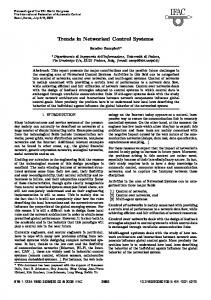
The first result is shown in Fig. 5. Circles and crosses represent the average delay in the event-triggered model and the periodic model, respectively. By “average”, we mean its total delay over N . From the plot, the periodic model introduced less delay than the event-triggered model, especially when N gets larger. In the event-triggered model, after N > 15, the delay increases quickly as the number of agents increases. We notice that when N = 15, the channel usage is 90% during the entire running time and when N ≥ 23, the channel occupation is 100%, which means agents always compete for the channel access. This is the indication that the bandwidth of the network is not high enough. Two reasons lead to the fast increase of delay. The first one is that as the number of agents increases, more agents compete for the channel access. The second reason is that, because every pendulum arm is connected to every other pendulum arm, the coefficient of the local error in the event is N δ. As N increases, the error becomes a larger weight, which leads to a short broadcast period.
performance different
20%
10%
0%
−10%
−20%
0
5
10
15
20 25 30 number of agents
35
40
45
50
Fig. 6. The performance comparison between the event-triggered model and the periodic model
The comparison of system performance in the event-triggered model and the periodic model is shown in Fig. 6. The vertical axis is p(t) defined in 33. When N = 3, the event-triggered model improves the performance by 20% compared with the periodic model. However, the improvement keeps decreasing as the number of agents increases until N = 30 when the performance of the event-triggered model becomes worse than the periodic model. Remember that when N ≥ 23, agents always compete for the channel access. In that case, event-triggering becomes meaningless since the agent’s decision is always broadcasting, not waiting. Therefore, when N is extremely large, the periodic model seems better since the periodic model introduces less delay into the system. This suggests that eventtriggered feedback, by itself, does not scale well with communication network density.
7
Conclusion
This paper examines event-triggered broadcasting of state information in distributed networked control systems. We showed that it is possible to design event-triggering thresholds that preserve asymptotic stability while only requiring “local” subsystem information to make their decisions. We showed that it is possible to design such thresholds using only local information about the dynamics of a subsystem. The approach applies to both nonlinear and linear systems, though determining the threshold for nonlinear systems requires the solution of a HJI inequality. For linear systems, this condition reduces to a much simpler LMI feasibility problem. We investigated the scalability of event-triggering through simulation studies. These results indicate that event-triggered systems outperform periodically triggered systems when there is little communication network congestion. As network density increases, thereby resulting in increased congestion, the performance of the event-triggered scheme begins to fall below
that achieved by the periodically triggered system. This suggests that eventtriggering, by itself, is not a scalable solution to networked feedback control systems. We firmly believe that the results indicate that broadcasting in such NCS requires a hybrid scheme that judiciously alternates between time-triggered and event-triggered broadcast strategies. Future work will investigate such hybrid schemes in a more rigorous manner.
References 1. Tabuada, P. and Wang, X.: Preliminary results on state-triggered scheduling of stabilizing control tasks. Proceedings of IEEE Conference on Decision and Control (2006). 2. Shin, K. G.,: Real-time communications in a computer-controlled workcell. IEEE Transactions on Robotics and Automation 7 (1991) 105–113 3. Zuberi, K. M., and Shin, K. G.,: Scheduling messages on controller area network for real-time CIM applications. IEEE Transactions on Robotics and Automation 13 (1997) 310–314 4. Krtolica R., and Ozguner U.,: Stability of linear feedback systems with random communication delays. Proceedings of American Control Conference (1991) 5. Wong, W. S., and Brockett, R. W.,: Systems with finite communication bandwidth constraints - Part I: State estimation problems. IEEE Transactions on Automatic Control 42 (1997) 1294–1299 6. Wong, W. S., and Brockett, R. W.,: Systems with finite communication bandwidth constraints - Part II: Stabilization with limited information feedback. IEEE Transactions on Automatic Control 44 (1999) 1049-1053 7. Walsh, G., Ye, H., and Bushnell, L.: Stability analysis of networked control systems. IEEE Transactions on Control Systems Technology, 10 (2002) 3 438–446 8. Zhang, W., Branicky, M., and Phillips, S.,: Stability of networked control systems. IEEE Control Systems Magazine, 21 (2001) 84–99 9. Sinopoli, B., Sharp, C., Schenato, L., Schaffert, S., and Sastry, S.,: Distributed control applications within sensor networks. Proceedings of the IEEE 91 (2003) 8 1235–1246 10. Gupta, P., and Kumar, P.,: The capacity of wireless networks. IEEE Transactions on Information Theory 46 (2000) 2 388–404 11. Arzen, K.,: A simple event-based pid controller. Proceedings of the 14th IFAC World Congress (1999). 12. Hristu-Varsakelis, D., and Kumar, P.,: Interrupt-based feedback control over a shared communication medium. Proceedings of the IEEE Conference on Decision and Control (2002) 13. Astrom, K., and Bernhardsson, B.: Comparison of riemann and lebesgue sampling for first order stochastic systems. Proceedings of the IEEE Conference on Decision and Control (1999) 14. Wang, X., and Lemmon, M.,:, Event-triggered Broadcasting across Distributed Networked Control Systems. submitted to American Control Conference (2008) 15. Wang, X., and Lemmon, M.,: Self-triggered feedback control systems with finitegain L2 stability. submitted to IEEE Transactions on Automatic Control (2007)