Decision Problems for Subclasses of Rational Relations over Finite ...

DMTCS vol. VOL:ISS, 2017, #NUM

Discrete Mathematics and Theoretical Computer Science

arXiv:1803.06140v1 [cs.FL] 16 Mar 2018

Decision Problems for Subclasses of Rational Relations over Finite and Infinite Words Christof Löding1 1 2

Christopher Spinrath2

RWTH Aachen University, Germany TU Dortmund University, Germany

received 1998-10-14, revised 2002-07-19, accepted 2015-09-09. We consider decision problems for relations over finite and infinite words defined by finite automata. We prove that the equivalence problem for binary deterministic rational relations over infinite words is undecidable in contrast to the case of finite words, where the problem is decidable. Furthermore, we show that it is decidable in doubly exponential time for an automatic relation over infinite words whether it is a recognizable relation. We also revisit this problem in the context of finite words and improve the complexity of the decision procedure to single exponential time. The procedure is based on a polynomial time regularity test for deterministic visibly pushdown automata, which is a result of independent interest. Keywords: rational relations, automatic relations, omega-automata, finite transducers, visibly pushdown automata

1 Introduction We consider in this paper algorithmic problems for relations over words that are defined by finite automata. Relations over words extend the classical notion of formal languages. However, there are different ways of extending the concept of regular language and finite automaton to the setting of relations. Instead of processing a single input word, an automaton for relations has to read a tuple of input words. The existing finite automaton models differ in the way how the components can interact while being read. In the following, we briefly sketch the four main classes of automaton definable relations, and then describe our contributions. A (nondeterministic) finite transducer (see, e.g., Berstel (1979); Sakarovitch (2009)) has a standard finite state control and at each time of a computation, a transition can consume the next input symbol from any of the components without restriction (equivalently, one can label the transitions of a transducer with tuples of finite words). The class of relations that are definable by finite transducers, referred to as the class of rational relations, is not closed under intersection and complement, and many algorithmic problems, like universality, equivalence, intersection emptiness, are undecidable (for details we refer to Rabin and Scott (1959)). A deterministic version of finite transducers defines the class of deterministic rational relations (see Sakarovitch (2009)) with slightly better properties compared to the nondeterministic version, in particular it has been shown by Bird (1973); Harju and Karhumäki (1991) that the equivalence problem is decidable. ISSN subm. to DMTCS

c 2017 by the author(s)

Distributed under a Creative Commons Attribution 4.0 International License

2

Christof Löding, Christopher Spinrath

Another important subclass of rational relations are the synchronized rational relations which have been studied by Frougny and Sakarovitch (1993) and are defined by automata that synchronously read all components in parallel (using a padding symbol for words of different length). These relations are often referred to as automatic relations, a terminology that we also adopt, and basically have all the good properties of regular languages because synchronous transducers can be viewed as standard finite automata over a product alphabet. These properties lead to applications of automatic relations in algorithmic model theory as a finite way of representing infinite structures with decidable logical theories (so called automatic structures, cf. Khoussainov and Nerode (1995); Blumensath and Grädel (2000)), and in regular model checking, a verification technique for infinite state systems (cf. Abdulla (2012)). Finally, there is the model of recognizable relations, which can be defined by a tuple of automata, one for each component of the relation, that independently read their components and only synchronize on their terminal states, i.e., the tuple of states at the end determines whether the input tuple is accepted. Equivalently, one can define recognizable relations as finite unions of products of regular languages. Recognizable relations play a role, for example, Bozzelli et al. (2015) use relations over words for identifying equivalent plays in incomplete information games. The task is to compute a winning strategy that does not distinguish between equivalent plays. While this problem is undecidable for automatic relations, it is possible to synthesize strategies for recognizable equivalence relations. In view of such results, it is an interesting question whether one can decide for a given relation whether it is recognizable. All these four concepts of automaton definable relations can directly be adapted to infinite words using the notion of ω-automata (see Thomas (1990) for background on ω-automata), leading to the classes of (deterministic) ω-rational, ω-automatic, and ω-recognizable relations. Applications like automatic structures and regular model checking have been adapted to relations over infinite words, e.g. by Blumensath and Grädel (2000); Boigelot et al. (2004), for instance for modeling systems with continuous parameters represented by real numbers (which can be encoded as infinite words, see e.g. Boigelot et al. (2005)). Our contributions are the following, where some background on the individual results is given below. We note that (4) is not a result on relations over words. It is used in the proof of (3) but we state it explicitly because we believe that it is an interesting result on its own. (1) We show that the equivalence problem for binary deterministic ω-rational relations is undecidable, already for the Büchi acceptance condition (which is weaker than parity or Muller acceptance conditions in the case of deterministic automata). (2) We show that it is decidable in doubly exponential time for an ω-automatic relation whether it is ω-recognizable. (3) We reconsider the complexity of deciding for a binary automatic relation whether it is recognizable, and prove that it can be done in exponential time. (4) We prove that the regularity problem for deterministic visibly pushdown automata — a model introduced by Alur and Madhusudan (2004) — is decidable in polynomial time. The algorithmic theory of deterministic ω-rational relations has not yet been studied in detail. We think, however, that this class is worth studying in order to understand whether it can be used in applications that are studied for ω-automatic relations. One such scenario could be the synthesis of finite state machines from (binary) ω-automatic relations. In this setting, an ω-automatic relation is viewed as a specification that relates input streams to possible output streams. The task is to automatically synthesize a

Decision Problems for Subclasses of Rational Relations

3

synchronous sequential transducer (producing one output letter for each input letter) that outputs a string for each possible input such that the resulting pair is in the relation (for instance, Thomas (2009) provides an overview of this kind of automata theoretic synthesis). It has recently been shown by Filiot et al. (2016) that this synchronous synthesis problem can be lifted to the case of asynchronous automata if the relation is deterministic rational. This shows that the class of deterministic rational relations has some interesting properties, and motivates our study of the corresponding class over infinite words. Our contribution (1) contrasts the decidability of equivalence for deterministic rational relations over finite words shown by Bird (1973); Harju and Karhumäki (1991) and thus exhibits a difference between deterministic rational relations over finite and over infinite words. We prove the undecidability by a reduction from the intersection emptiness problem for deterministic rational relations over finite words. The reduction is inspired by a recent construction of Böhm et al. (2017) for proving the undecidability of equivalence for deterministic Büchi one-counter automata. Contributions (2) and (3) are about the effectiveness of the hierarchies formed by the four classes of (ω-)rational, deterministic (ω-)rational, (ω-)automatic, and (ω-)recognizable relations. A systematic overview and study on the effectiveness of this hierarchy for finite words is provided by Carton et al. (2006): For a given rational relation it is undecidable whether it belongs to one of the other classes, for deterministic rational and automatic relations it is decidable whether they are recognizable, and the problem of deciding for a deterministic rational relation whether it is automatic is open. The question of the effectiveness of the hierarchy for relations over infinite words has already been posed by Thomas (1992) (where the ω-automatic relations are called Büchi recognizable ω-relations). The undecidability results easily carry over from finite to infinite words. Our result (2) lifts one of the two known decidability results for finite words to infinite words. The algorithm is based on a reduction to a problem over finite words: Using a representation of ω-languages by finite encodings of ultimately periodic words as demonstrated by Calbrix et al. (1993), we are able to reformulate the recognizability of an ω-automatic relation in terms of slenderness of a finite number of languages of finite words. We adopt the term slender from Pˇaun and Salomaa (1995). A language of finite words is called slender if there is a bound k such that the language contains for each length at most k words of this length. While slenderness for regular languages is easily seen to be decidable, the complexity of the problem has to the best of our knowledge not been analyzed. We prove that slenderness of a language defined by a nondeterministic finite automaton can be decided in NL. As mentioned above, the decidability of recognizability of an automatic relation has already been proved by Carton et al. (2006). However, the exponential time complexity claimed in that paper does not follow from the proof presented there. So we revisit the problem and prove the exponential time upper bound for binary relations based on the connection between binary rational relations and pushdown automata: For a relation R over finite words, consider the language LR consisting of the words rev(u)#v for all (u, v) ∈ R, where rev(u) denotes the reverse of u. It turns out that LR is linear context-free iff R is rational, LR is deterministic context-free iff R is deterministic rational, and LR is regular iff R is recognizable (cf. Carton et al. (2006)). Since LR is regular iff R is recognizable, the recognizability test for binary deterministic rational relations reduces to the regularity test for deterministic pushdown automata, which has been shown to be decidable by Stearns (1967). Valiant (1975) improved this decidability result for deterministic pushdown automata by proving a doubly exponential upper bound.(i) We (i)

Recognizability is decidable for deterministic rational relations of arbitrary arity as shown by Carton et al. (2006) but we are not aware of a proof preserving the doubly exponential runtime.

4


adapt this technique to automatic relations R and show that LR can in this case be defined by a visibly pushdown automaton (VPA) (see Alur and Madhusudan (2004)), in which the stack operation (pop, push, skip) is determined by the input symbol, and no ε-transitions are allowed. The deterministic VPA for LR is exponential in the size of the automaton for R, and we prove that the regularity test can be done in polynomial time, our contribution (4). We note that the polynomial time regularity test for visibly pushdown processes as presented by Srba (2006) does not imply our result. The model used by Srba (2006) cannot use transitions that cause a pop operation when the stack is empty. For our translation from automatic relations to VPAs we need these kind of pop operations, which makes the model different and the decision procedure more involved (and a reduction to the model of Srba (2006) by using new internal symbols to simulate pop operations on the empty stack will not preserve regularity of the language, in general). This paper is the full version of the conference paper of Löding and Spinrath (2017). In contrast to the conference version, which only sketches proof ideas for the major results, it contains full proofs for all (intermediate) results. Furthermore, Section 4 is enriched by an example which illustrates why the exponential time complexity claimed by Carton et al. (2006) does not follow from their proof approach. Also, we give an additional comment on the connection of the properties slenderness – which we exhibit to show the decidability of recognizability for ω-automatic relations – and finiteness – used in the approach of Carton et al. (2006) to show the decidability of recognizability of automatic relations. The paper is structured as follows. In Section 2 we give the definitions of transducers, relations, and visibly pushdown automata. In Section 3 we prove the undecidability of the equivalence problem for deterministic ω-rational relations. Section 4 contains the decision procedure for recognizability of ωautomatic relations, and Section 5 presents the polynomial time regularity test for deterministic VPAs and its use for the recognizability test of automatic relations. Finally, we conclude in Section 6.

2 Preliminaries We start by briefly introducing transducers and visibly pushdown automata as we need them for our results. For more details we refer to Sakarovitch (2009); Frougny and Sakarovitch (1993); Thomas (1990) and Alur and Madhusudan (2004); Bárány et al. (2006), respectively.

2.1 Finite Transducers and (ω-)Rational Relations A transducer A is a tuple (Q, Σ1 , . . . , Σk , q0 , ∆, F ) where Q is the state set, Σi , 1 ≤ i ≤ k are (finite) alphabets, q0 ∈ Q is the initial state, F ⊆ Q denotes the accepting states, and ∆ ⊆ Q × (Σ1 ∪{ε})× . . .× (Σk ∪ {ε}) × Q is the transition relation. A is deterministic if there is a state partition Q = Q1 ∪ . . . ∪ Qk Sk such that ∆ can be interpreted as partial function δ : j=1 (Qj × (Σj ∪ {ε})) → Q with the restriction that if δ(q, ε) is defined then no δ(q, a), a 6= ε is defined. Note that the state determines which component the transducer processes. A is complete if δ is total (up to the restriction for ε-transitions). A run of A on a tuple u ∈ Σ∗1 × . . . × Σ∗k is a sequence ρ = p0 . . . pn ∈ Q∗ such that there is a decomposition u = (a1,1 , . . . , a1,k ) . . . (an,1 , . . . , an,k ) where the ai,j are in Σj ∪ {ε} and for all i ∈ {1, . . . , n} it holds that (pi−1 , ai,1 , . . . , ai,k , pi ) ∈ ∆. The run of A on a tuple over infinite words ω ω in Σω 1 × . . . × Σk is an infinite sequence p0 p1 . . . ∈ Q defined analogously to the case of finite words. u1 /.../uk u We use the shorthand notation A : p −−−−−−→ q or A : p − → q to denote the existence of a run of A ∗ on u = (u1 , . . . , uk ), uj ∈ Σj starting in p and ending in q. Concerning runs on tuples of infinite words vi u v u q)i≥0 or p − → (q − → q)ω if we deliberately extend this notation in the natural way and write p − → (q −→


5

both, the run and the input tuple, permit it. A run on u is called accepting if it ends in an accepting state and A accepts u if there is an accepting run starting in the initial state q0 . Then A defines the relation R∗ (A) ⊆ Σ∗1 ×. . .×Σ∗k containing precisely those tuples accepted by A. To enhance the expressive power of deterministic transducers, the relation R∗ (A) is defined as the relation of all u such that A accepts Sk u(#, . . . , #) for some fresh fixed symbol # ∈ / j=1 Σj . The relations definable by a (deterministic) ω transducer are called (deterministic) rational relations. For tuples over infinite words u ∈ Σω 1 × . . . × Σk ω we utilize the Büchi condition (cf. Büchi (1962)). That is, a run ρ ∈ Q is accepting if a state f ∈ F occurs infinitely often in ρ. Then A accepts u if there is an accepting run of A on u starting in q0 and ω Rω (A) ⊆ Σω 1 × . . . × Σk is the relation of all tuples of infinite words accepted by A. We refer to A as Büchi transducer if we are interested in the relation of infinite words defined by it. The class of ω-rational relations consists of all relations definable by Büchi transducers. It is well-known that deterministic Büchi automata are not sufficient to capture the ω-regular languages (see Thomas (1990)) which are the ω-rational relations of arity one. Therefore, we use another kind of transducer to define deterministic ω-rational relations: a deterministic parity transducer is a tuple A = (Q, Σ1 , . . . , Σk , q0 , δ, Ω) where the first k + 3 items are the same as for deterministic transducers and Ω : Q → N is the priority function. A run is accepting if the maximal priority occurring infinitely often on the run is even (cf. Piterman (2006)). A transducer is synchronous if for each pair (p, a1 , . . . , ak , q), (q, b1 , . . . , bk , r) of successive transitions it holds that aj = ε implies bj = ε for all j ∈ {1, . . . , k}. Intuitively, a synchronous transducer is a finite automaton over the vector alphabet Σ1 × . . . × Σk and, if it operates on tuples (u1 , . . . , uk ) of finite words, the components uj may be of different length (i.e. if a uj has been processed completely, the transducer may use transitions reading ε in the j-th component to process the remaining input in the other components). In fact, synchronous transducers inherit the rich properties of finite automata – e.g., they are closed under all boolean operations and can be determinized. In particular, synchronous (nondeterministic) Büchi transducer and deterministic synchronous parity transducer can be effectively transformed into each other (see Sakarovitch (2009); Frougny and Sakarovitch (1993); Piterman (2006)). Synchronous (Büchi) transducers define the class of (ω-)automatic relations. Finally, the last class of relations we consider are (ω-)recognizable relations. A relation R ⊆ Σ∗1 ×. . .× ω ∗ Σk (or R ⊆ Σω 1 × . . . × Σk ) is (ω-)recognizable if it is the finite union of direct products of (ω-)regular Sℓ languages — i.e. R = i=1 Li,1 × . . . × Li,k where the Li,j are (ω-)regular languages. It is well-known that the classes of (ω-)recognizable, (ω-)automatic, deterministic (ω-)rational relations, and (ω-)rational relations form a strict hierarchy (see Sakarovitch (2009)).

2.2 Visibly Pushdown Automata In Section 5, we use visibly pushdown automata (VPAs) which have been introduced by Alur and Madhusudan (2004). They operate on typed alphabets, called pushdown alphabets below, where the type of input symbol determines the stack operation. Formally, a pushdown alphabet is an alphabet Σ consisting of three disjoint parts — namely, a set Σc of call symbols enforcing a push operation, a set Σr of return symbols enforcing a pop operation and internal symbols Σint which do not permit any stack operation. A VPA is a tuple P = (P, Σ, Γ, p0 , ⊥, ∆, F ) where P is a finite set of states, Σ = Σc ∪˙ Σr ∪˙ Σint is a finite pushdown alphabet, Γ is the stack alphabet and ⊥ ∈ Γ is the stack bottom symbol, p0 ∈ P is the initial state, ∆ ⊆ (P × Σc × P × (Γ \ {⊥})) ∪ (P × Σr × Γ × P ) ∪ (P × Σint × P ) is the transition relation, and F is the set of accepting states.

6


A configuration of P is a pair in (p, α) ∈ P × (Γ \ {⊥})∗ {⊥} where p is the current state of P and α is the current stack content (α[0] is the top of the stack). Note that the stack bottom symbol ⊥ occurs precisely at the bottom of the stack. The stack whose only content is ⊥, is called the empty stack. P can proceed from a configuration (p, α) to another configuration (q, β) via a ∈ Σ if a ∈ Σc and there is a (p, a, q, γ) ∈ ∆ ∩ (P × Σc × P × (Γ \ {⊥})) such that β = γα (push operation), a ∈ Σr and there is a (p, a, γ, q) ∈ ∆ ∩ (P × Σr × Γ × P ) such that α = γβ or γ = α = β = ⊥ — that is, the empty stack may be popped arbitrarily often (pop operation), or a ∈ Σint and there is a (p, a, q) ∈ ∆ ∩ (P × Σint × P ) such that α = β (noop). A run of P on a word u = a1 , . . . , an ∈ Σ∗ is a sequence of configurations (p1 , α1 ) . . . (pn+1 , αn+1 ) connected by transitions using the corresponding u input letter. As for transducers we use the shorthand P : (p1 , α1 ) − → (pn+1 , αn+1 ) to denote a run. A run is accepting if pn+1 ∈ F . Furthermore, we say that P accepts u if (p1 , α1 ) is the initial configuration (p0 , ⊥) and write L(p, α) for the set of all words accepted from a configuration (p, α). In the case (p, α) = (p0 , ⊥) we just say that P accepts u and write L(P) := L(p0 , ⊥) for the language defined by P. Two configurations (p, α), (q, β) are P-equivalent if L(p, α) = L(q, β). We denote the P-equivalence relation by ≈P . That is, (p, α) ≈P (q, β) if and only if L(p, α) = L(q, β). Lastly, a configuration (p, α) is reachable if there is a run from (p0 , ⊥) to (p, α). A deterministic VPA (DVPA) P is a VPA that can proceed to at most one configuration for each given configuration and a ∈ Σ. Viewing the call symbols as opening and the return symbols as closing parenthesis, one obtains a natural notion of a return matching a call, and unmatched call or return symbols. Furthermore, we need the notion of well-matched words (cf. Bárány et al. (2006)). The set of well-matched words over a pushdown alphabet Σ is defined inductively by the following rules: • Each w ∈ Σ∗int is a well-matched word. • For each well-matched word w, c ∈ Σc and r ∈ Σr the word cwr is well-matched. • Given two well-matched words w, v their concatenation wv is well-matched. An important observation regarding well-matched words is that the behavior of P on a well-matched word w is invariant under the stack content. That is, for any configurations (p, α), (p, β) we have that w w P : (p, α) − → (q, α) if and only if P : (p, β) − → (q, β). In particular, this holds true for the empty stack u ∗ α = ⊥. Furthermore, every word u ∈ Σ with P : (q0 , α) − → (pn+1 , γn . . . γ1 α) for some γn , . . . , γ1 ∈ Γ \ {⊥}, n ≤ |u| can be decomposed into well-matched words w1 , . . . , wn+1 and c1 , . . . , cn ∈ Σc such that u = w1 c1 w2 . . . cn wn+1 . Moreover, there are configurations (p1 , α), (q1 , γ1 α), . . . , (pn , γn−1 . . . γ1 α), (qn , γn . . . γ1 α) such that w

c

i i (qi , γi . . . γ1 α) (pi , γi−1 . . . γ1 α) −→ (qi−1 , γi−1 . . . γ1 α) −→

holds. Informally, the symbol ci is responsible for pushing γi onto the stack. A similar decomposition is possible for words u popping a sequence γn . . . γ1 from the top of the stack. In that case we have that the word u factorizes into u = w1 r1 . . . rn wn+1 where the wj are well-matched words and the ri are from Σr . Also, the symbol ri is responsible for popping γi .


7

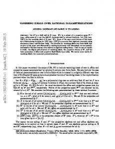
3 The Equivalence Problem for Deterministic Buchi ¨ Transducers In this section we show that the equivalence for deterministic Büchi transducers is undecidable – in difference to its analogue for relations over finite words proven by Bird (1973); Harju and Karhumäki (1991). Our proof is derived from a recent construction by Böhm et al. (2017) for proving that the equivalence problem for one-counter Büchi automata is undecidable. We reduce the intersection emptiness problem for relations over finite words to the equivalence problem for deterministic Büchi transducers. Proposition 1 (Rabin and Scott (1959); Berstel (1979)). The intersection emptiness problem, asking for two binary relations given by deterministic transducers A, B whether R∗ (A) ∩ R∗ (B) = ∅ holds, is undecidable. Theorem 2. The equivalence problem for ω-rational relations of arity at least two is undecidable for deterministic Büchi transducers. Proof: We prove Theorem 2 by providing a many-one-reduction from the emptiness intersection problem over finite relations to the equivalence problem for deterministic ω-rational relations. Then the claim follows due to the undecidability of the emptiness intersection problem (cf. Proposition 1). Furthermore, it suffices to provide the reduction for relations of arity k = 2. For k > 2 the claim follows by adding dummy components to the relation. Let AR , AS be deterministic transducers defining binary relations R and S over finite words, respectively. More precisely, we let AR = (QR , Σ1 , Σ2 , q0R , δR , FR ) and AS = (QS , Σ1 , Σ2 , q0S , δS , FS ). We construct deterministic Büchi transducers BR and BS such that R ∩ S 6= ∅ ⇔ Rω (BR ) 6= Rω (BS ). That is, each tuple in R ∩ S induces a witness for Rω (BR ) 6= Rω (BS ) and vice versa. Recall that AR , AS accept a tuple (u, v) if there is an accepting run on (u, v)(#, #) (where # is an endmarker symbol not contained in any alphabet involved). Then it is easy to see that we can assume that the deterministic transducers AR and AS are in normal form according to Sakarovitch (2009): the initial states q0R and q0S do not have incoming transitions and there are unique accepting states qaR and qaS as well as rejecting states qrR and qrS that 1. are entered only by transitions labeled #, and 2. have no outgoing transitions. That is, we have that FR = {qaR } and upon the end of any run AR is either in state qaR or qrR 6= qaR after reading the endmarker # in both components. Analogously, the same applies for AS . The construction of BR and BS is illustrated in Figure 1. Both Büchi transducers are almost the same except for the initial state: both consist of the union of the transition structures of AR and AS complemented by transitions labeled ε/ε from qaX to q0X and qrX to q0Y for X, Y ∈ {R, S}, X 6= Y . That is, upon reaching a rejecting state of AR or AS the new transducers will switch to the initial state of the other subtransducer(ii) and upon reaching an accepting state they will return to the initial state of the current (ii)

For our purpose, a subtransducer of B is a transducer obtained from B by removing states and transitions. Also, accepting states do not have to be preserved. In particular, AR and AS are subtransducers of BR and BS by definition.

8


subtransducer. The new accepting states are qaR , qrR , qrS . Note that qaS is not accepting introducing an asymmetry. Finally, the initial state of BX is q0X . Formally, we set BR := (QB , Σ′1 , Σ′2 , q0R , δB , FB ) and BS := (QB , Σ′1 , Σ′2 , q0S , δB , FB ) where • QB := QR ∪˙ QS , • Σ′i := Σi ∪ {#}, i ∈ {1, 2}, and • FB := {qaR , qrR , qrS }. The transition relation δB is defined as follows:  δR (q, a),    δ (q, a), S δB (q, a) := S  δ   S (q0 , a),  δR (q0R , a),

q q q q

∈ QR \ {qaR , qrR } ∈ QS \ {qaS , qrS } ∈ {qrR , qaS } ∈ {qrS , qaR }

Further on, we show the correctness of our construction. Pick a tuple (u, v) in R ∩ S. We have to show that Rω (BR ) 6= Rω (BS ). Then the unique runs of AR and AS on (u#, v#) end in qaR and qaS , respectively: u#/v#

u#/v#

AR : q0R −−−−−→ qaR and AS : q0S −−−−−→ qaS . Recall that qaR and qaS have precisely the same transitions as q0R and q0S , respectively. Thus, they have the same behavior. Hence, the unique runs of BR and BS on w := (u#, v#)ω , which are completely determined by AR and AS , have the following shape: ω ω R R u#/v# R u#/v# S S u#/v# S u#/v# BR : q0 −−−−−→ qa −−−−−→ qa and BS : q0 −−−−−→ qa −−−−−→ qa . Since qaR ∈ FB , it follows that w ∈ Rω (BR ). On the other hand, the run of BS stays completely in the AS subtransducer and qrS does not occur in it. Assuming otherwise, AS would reject (u, v) which would be a contradiction. But then no state in FB occurs in the run of BS (recall that in contrast to qaR the state qaS is not in FB ). Hence, w ∈ / Rω (BS ). Therefore, the induced unique run of BR on (u#, v#)ω is accepting while the unique run of BS is rejecting. Thus, w ∈ Rω (BR ) \ Rω (BS ) and we can conclude that Rω (BR ) 6= Rω (BS ) holds. For the other direction, suppose Rω (BR ) 6= Rω (BS ) holds. Then there is a pair of infinite words (u, v) that is rejected by one of the transducers, and accepted by the other. Recall that the accepting states of both BR and BS can only be entered by reading the #-symbol in both components. Hence, both components of (u, v) have to contain infinitely often #, since one of the Büchi transducers accepts. More precisely, the pair (u, v) can be written as (u, v) = (u0 , v0 )(#, #)(u1 , v1 )(#, #) . . . ∈ Rω (BR )△Rω (BS ), with (ui , vi ) ∈ Σ∗1 × Σ∗2 ∀i ∈ N. We claim that there is a p ∈ N such that (up , vp ) ∈ R ∩ S. Then R ∩ S 6= ∅ follows immediately.

9


Let ρR and ρS be the unique runs of BR and BS , respectively. W.l.o.g. assume that BR rejects (u, v) while BS accepts it. In the other case the reasoning is exactly the same with BR and BS exchanged. Since ρR is not accepting, the states in FB occur only finitely often in ρR . On the other hand, the endmarker # is read infinitely often. Thus, states in FB ∪ {qaS } occur infinitely often because they are entered if and only if endmarkers have been read in both components. It follows that ρR stays in the AS subtransducer from some point on and qaS occurs infinitely often in ρR . To be more precise, qaS does occur precisely after reading the endmarker in both components and, afterwards, continue the run in AS . All in all, the run is determined by run fragments u0 #u1 #...uj−1 #/v0 #v1 #...vj−1 #

uj #/vj #

ui #/vi #

q0R −−−−−−−−−−−−−−−−−−−−−−→ q0S −−−−−−→ qaS and qaS −−−−−−→ qaS for some j ∈ N and all i > j. Hence, it holds that ∃j ≥ 0 ∀i ≥ j : (ui , vi ) ∈ S

(⋆)

because AS and BR are deterministic and, by construction, qaS imitates q0S . Further on, it suffices to show that ρS (the unique accepting run of BS ) stays in AR from some point on. Then it follows analogously to the case for ρR that (⋆) holds for R and, thus, we have that (up , vp ) ∈ R ∩ S for some p. First of all, ρS does not stay in AS from some point on. Otherwise, it would not be accepting. Assume for the sake of contradiction that the run ρS switches infinitely often between the two subtransducers, i.e. both qrS and qrR occur infinitely often in the run. It follows that ρS contains infinitely many fragments of the form ui #/vi #

ui #/vi #

qrR −−−−−−→ qrS or qaS −−−−−−→ qrS where all intermediate states are in QS . Thus, because qrR and qaS behave in the same way as q0S by construction and AS is deterministic, we have that ∀j ≥ 0 ∃i ≥ j : (ui , vi ) ∈ / S. But this is a direct contradiction to (⋆). Hence, ρS stays in the AR subtransducer from some point on, and similarly to the case for ρR above, it follows that ∃j ≥ 0 ∀i ≥ j : (ui , vi ) ∈ R.

(⋆⋆)

Let p ∈ N the maximum of the existentially quantified j’s in (⋆) and (⋆⋆). Then we have that (up , vp ) ∈ R ∩ S 6= ∅. All in all, we have shown that R ∩ S 6= ∅ ⇔ Rω (BR ) 6= Rω (BS ) holds and, thus, the correctness of our reduction. We note that our reduction is rather generic an could be applied to other classes of automata for which the intersection emptiness problem on finite words is undecidable.

4 Deciding Recognizability of ω-Automatic Relations Our aim in this section is to decide ω-recognizability of ω-automatic relations in doubly exponential time. That is, given a deterministic synchronous transducer, decide whether it defines an ω-recognizable

10


AR

AS ε/ε

BR

q0R

...

#/#

qaR

ε/ε

... ...

BS #/#

qrR

q0S

...

qaS

... ...

ε/ε

#/#

#/#

qrS

ε/ε Fig. 1: Illustration of the transducers BR , BS . The labels #/# are just used for comprehensibility. In the formal construction the # symbols are read in succession and the transducers may even read other symbols between them (but only in the component where no # has been read yet).

relation. The proof approach is based on an algorithm for relations over finite words given by Carton et al. (2006) which we briefly discuss in Subsection 4.1. Afterwards, in Subsection 4.2, we present our main result of this section. In Subsection 4.3, we comment on a connection between Carton et al. (2006)’s original proof and our (alternative) approach for infinite words.

4.1 Revision: Deciding Recognizability of Automatic Relations Let R be an (ω-)automatic relation of arity k. For each j ≤ k we define the equivalence relation Ej := {((u1 , . . . , uj ), (v1 , . . . , vj )) | ∀wj+1 , . . . , wk : (u1 , . . . , uj , wj+1 , . . . , wk ) ∈ R ⇔ (v1 , . . . , vj , wj+1 , . . . , wk ) ∈ R}. Then the key to decide (ω-)recognizability is the following result which has been proven by Carton et al. (2006) for relations over finite words and is easily extensible to infinite words: Lemma 3 (Carton et al. (2006)). Let R be an (ω-)automatic relation of arity k. Then for all 1 ≤ j ≤ k the equivalence relation Ej has finite index if and only if R is (ω-)recognizable. Here we shall adapt the proof of Carton et al. (2006) to ω-automatic relations. Sℓ Proof: ⇒: Assume R 6= ∅ is ω-recognizable. Then we have that R = i=1 Li,1 × . . . × Li,k for some ωω regular languages Li,n ⊆ Σω n . Pick words ui ∈ Li,1 for all i ∈ {1, . . . , ℓ}. Then each word in Σ1 is either equivalent w.r.t. E1 to one of these ui or belongs to the equivalence class Σω \ dom(R). Thus, E1 has 1 finite index. The proof for Ej , j > 1 works similarly by picking tuples (ui,1 , . . . , ui,j ) ∈ Li,1 ×. . .×Li,j . ⇐: Assume all Ej have finite index. We show the claim by induction over k. For the base case of a 1-ary ω-rational relation the claim is trivial. Suppose that k ≥ 2. We prove that R can be written as finite union of direct products of ω-regular languages. Then it follows by definition that R is recognizable. Recall that dom(R) is ω-regular. Hence, we can pick an ultimately periodic word u1 ∈ dom(R) (cf. Büchi (1962)). Clearly, {u1 } × Σω 1 is ω-automatic. Furthermore, since ω-automatic relations are closed under intersection (and E1 itself is ω-automatic) it holds that ω E1 ∩ ({u1 } × Σω 1 ) = {u1 } × {w ∈ Σ1 | (u1 , w) ∈ E1 } = {u1 } × [u1 ]E1


11

is ω-automatic. In particular, it follows that the equivalence class of u1 , denoted [u1 ]E1 , is ω-regular. ω Moreover, each {u1 } × Σω 2 × . . . × Σk is ω-recognizable. Hence, the relation ω R|u1 := {(x2 , . . . , xk ) | (u1 , x2 , . . . , xk ) ∈ R} ⊆ Σω 2 × . . . × Σk

is ω-automatic. By iteratively applying this reasoning to dom(R)\[u1 ]E1 we obtain a sequence u1 , u2 , . . . such that all ui are pairwise non-equivalent ultimately periodic representatives. Since E1 has finite index by assumption, this sequence is finite. Observe that this implies that R can be written as the finite union Sℓ R = i=1 [ui ]E1 × R|ui . Recall that the R|ui are ω-automatic. Hence, it suffices to show that for each R|u1 the induced equivalence relations have all finite index. Then the claim follows by the induction hypothesis. For this purpose, observe that an equivalence class of some Ej is solely determined by a set of possible outputs. More precisely, for T := R|u1 and all 2 ≤ j ≤ k we have that T |v2 ,...,vj = {(vj+1 , . . . , vk ) | (v2 , . . . , vk ) ∈ T } = {(vj+1 , . . . , vk ) | (ui , v2 , . . . , vk ) ∈ R} = R|ui ,v2 ,...,vj . Therefore, it follows by the definition of the Ej that for all R|ui the induced equivalence relations have all finite index. Based on that lemma, the recognizability test presented by Carton et al. (2006) proceeds as follows. It is shown that each Ej is an automatic equivalence relation by constructing a synchronous transducer for Ej . It remains to decide for an automatic equivalence relation whether it is of finite index. This can be achieved by constructing a synchronous transducer that accepts a set of representatives of the equivalence classes of Ej (based on a length-lexicographic ordering). Then Ej has finite index if and only if this set of representatives is finite, which can be decided in polynomial time. It is unclear whether this approach can be used to obtain an exponential time upper bound for the recognizability test.(iii) One can construct a family (Rn )n∈N of automatic binary relations Rn defined by a deterministic synchronous transducer of size O(n2 ) such that every synchronous transducer defining E1 has size (at least) exponential in n (cf. Example 4). It is unclear whether it is possible to decide in polynomial time for such a transducer whether the equivalence relation it defines is of finite index. For this reason, we revisit the problem for finite words in Section 5 and provide an exponential time upper bound for binary relations using a different approach. Example 4. We construct for any n ∈ N an automatic (binary) relation Rn in terms of a deterministic synchronous transducer of size O(n2 ) such that every synchronous transducer defining E1 has size (at least) exponential in n. Let n ∈ N and Σ := {0, 1}. Consider the relation Rn := {(u#v, t) | u, v, t ∈ Σn , |t|1 ≤ 1, ∀0 ≤ i < n : t[i] = 1 → u[i] = v[i]} That is, Rn consists of tuples (u#v, t) where u, v and t are bit strings of length n and t contains at most one 1. Moreover, the occurrence of this 1 (if present) marks a position where u and v are equal. A deterministic synchronous transducer An can define Rn with the help of two finite counters ranging over {0, . . . , n} as follows: the first counter measures the length of u and t and the second counter determines the position of the 1-symbol in the second component t (if present). Initially, both counters are (iii)

Carton et al. (2006) mainly focused on decidability, and they agree that the proof as presented in that paper does not yield an exponential time upper bound.

12


increased by one on each transition of An . Whether the second component is malformed (i.e. contains two 1’s), is verifiable with a single control bit in the state space. Also, An can remember the bit indicated by a 1 in the second component with a single bit in the state space and stop the second counter (containing the correct position of the 1). Up on reaching the separator # in the first component, An resets the first counter (assuming the input has been well-formed so far; otherwise, it rejects) and utilizes it to verify the length of v. Moreover, it decreases the second counter on each transition. If 0 is reached it has found the position i in v marked by the second component and can compare v[i] with u[i] which has been saved in the state space. Finally, the case that the second counter does not stop (i.e. there is no 1 in the second component) can be handled with another control bit in the state space. An has to store both counters plus finitely many control/memory bits (whose number is independent of n) in the state space. Hence, Rn is definable by a deterministic synchronous transducer of size O(n2 ). It remains to show that every transducer defining E1 has size exponential in n. For each input u#v ∈ Σn {#}Σn it holds that(iv) R|u#v = R(u#v) = {0i 10n−i−1 | 0 ≤ i < n, (u ⊕ v)[i] = 0} ∪ {0n }. It suffices to show that every transducer recognizing 2 E1′ := E1 ∩ Σn {#}Σn = {(u#v, u′ #v ′ ) | u, v, u′ , v ′ ∈ Σn ∧ ∀ 0 ≤ i < n : (u ⊕ v)[i] = (u′ ⊕ v ′ )[i]} 2 has size exponential in n. This holds because Σn {#}Σn is definable by a deterministic synchronous transducer of size O(n). Note that the existence of a synchronous transducer of sub-exponential size for E1 would imply the existence of one for the intersection. Furthermore, observe that we cut out all pairs of malformed inputs x ∈ (Σ ∪ {#})∗ — i.e. with R(x) = ∅. For the sake of contradiction, suppose there is synchronous transducer Bn = (Q, Σ, Σ, q0 , ∆, F ) defining E1′ with |Q| < 2n . By the pigeonhole principle there are i ∈ n, p ∈ Q and u, u′ , x, x′ , v, v ′ , y, y ′ ∈ Σn such that (u ⊕ u′ )[i] 6= (x ⊕ x′ )[i] and u#/u′ #

v/v ′

x#/x′ #

y/y ′

Bn : q0 −−−−−→ p −−−→ F as well as Bn : q0 −−−−−→ p −−−→ F. In particular, u#v and u′ #v ′ as well as x#y and x′ #y ′ are equivalent. Moreover, x#v and x′ #v ′ are equivalent, too, since B permits an accepting run. W.l.o.g. we have that (u⊕u′ )[i] = 0 and (x⊕x′ )[i] = 1. That is, u[i] = u′ [i] and x[i] 6= x′ [i]. Thus, (u ⊕ v)[i] = (u′ ⊕ v)[i] = (u′ ⊕ v ′ )[i]. We deduce v[i] = v ′ [i]. Then, similarly to the previous reasoning, we have that (x ⊕ v)[i] = (x ⊕ v ′ )[i] = (x′ ⊕ v ′ )[i]. But this yields x[i] = x′ [i] which is a contradiction to (x ⊕ x′ )[i] = 1. Thus, every deterministic transducer defining Ej′ has size at least 2n which proves the lemma.

4.2 From Indices of Equivalence Relations to Slenderness of Languages We now turn to the case of infinite words. The relation Ej can be shown to be ω-automatic, similarly to the case of finite words. However, it is not possible, in general, for a given ω-automatic relation to define a set of representatives by means of a synchronous transducer, as shown by Kuske and Lohrey (2006): There exists a binary ω-automatic equivalence relation such that there is no ω-regular set of representatives of the equivalence classes. (iv)

u ⊕ v shall denote the bitwise XOR operation on u and v.


13

Here is how we proceed instead. The first step is similar to the approach of Carton et al. (2006): We construct synchronous transducers for the complements Ej of the equivalence relations Ej in polynomial time (starting from a deterministic transducer for R). We then provide a decision procedure to decide for a given transducer for Ej whether the index of Ej is finite in doubly exponential time. This procedure is based on an encoding of ultimately periodic words by finite words. ω First observe that a tuple in Σω 1 × . . . × Σj can be seen as an infinite word over Σ = Σ1 × . . . × Σj (this is not the case for tuples over finite words, since the words may be of different length). Hence, we can view each Ej as a binary equivalence relation E ⊆ Σω × Σω . For this reason, we only work with binary relations in the following. We start by showing that for deciding whether E has finite index it suffices to consider sets of ultimately periodic representatives ui viω such that the periods |vi | and prefix lengths |ui | are the same, respectively, for all the representatives (Lemma 6). In the second step E is transformed into an automatic equivalence relation E# over finite words using encodings of ultimately periodic words as finite words, where a word uv ω is encoded by u#v as done by Calbrix et al. (1993) (Definition 8 and Lemma 9). Since E# is an automatic relation over finite words, it is possible to obtain a finite automaton for a set of representatives of E# . Finally, we reduce the decision problem whether E has finite index to deciding slenderness (see Definition 5 below) for polynomially many languages derived from the set of representatives of E# (Lemmas 12 & 13). Therefore, by proving that deciding slenderness for (nondeterministic) finite automata is NL-complete (Lemma 14) we obtain our result. Definition 5 (Pˇaun and Salomaa (1995)). A language L ⊂ Σ∗ is slender if there exists a k < ω such that for all ℓ < ω it holds that |L ∩ Σℓ | < k. We now formalize the ideas sketched above. Lemma 6. Let E ⊆ Σω × Σω be an ω-automatic equivalence relation. Then E has not finite index if and only if for each k > 0 there are u1 , . . . , uk , v1 , . . . vk ∈ Σ∗ with |ui | = |uj | and |vi | = |vj | for all 1 ≤ i ≤ j ≤ k such that (ui viω , uj vjω ) ∈ / E for all 1 ≤ i < j ≤ k. To prove Lemma 6 we first show the following, slightly weaker, version of it: Lemma 7. Let E ⊆ Σω × Σω be a ω-automatic equivalence relation. Then E has not finite index if and only if there are infinitely many (pairwise different) equivalence classes of E containing an ultimately periodic representative. Proof: ⇐: Indeed, if E has finite index then there are only finitely many equivalence classes of E (containing an ultimately periodic word) by definition. ⇒: Suppose E has not finite index. For the sake of contradiction assume that there are only n < ω equivalence classes containing an ultimately periodic representative. We show that E has only finitely many equivalence classes at all which contradicts the premise. Let ui viω ∈ Σω , 1 ≤ i ≤ n be fixed ultimately periodic representatives of those finitely many equivalence classes containing an ultimately periodic representative — i.e. for each ultimately periodic word uˆvˆω ∈ Σω we have that (ˆ uvˆω , ui viω ) ∈ E ω ω for exactly one 1 ≤ i ≤ n. Clearly, {ui vi } × Σ is ω-automatic. Furthermore, since ω-automatic relations are closed under intersection (and E itself is ω-automatic) it holds that E ∩ ({ui viω } × Σω ) = {ui viω } × {w ∈ Σω | (ui viω , w) ∈ E} = {ui viω } × [ui viω ]E

14


Sk is ω-automatic for all 1 ≤ i ≤ k. Lastly, T := i=1 [ui viω ]E ⊆ Σω is ω-automatic because of the closure under projection and finite unions. We claim that T = dom(E). Obviously, for each w ∈ Σω we have that (w, w) ∈ E, and, hence, T ⊆ dom(E) = Σω . Assume that dom(E) \ T is non-empty. It follows that dom(E) \ T (which is ω-automatic again) contains an ultimately periodic word u ˆvˆω (cf. Büchi (1962)). By the choice of the ω ω ω ui vi there is an 1 ≤ i ≤ n such that u ˆvˆ ∈ [ui vi ]E ⊆ T which contradicts uˆvˆω ∈ dom(E) \ T . Thus, dom(E) \ T 6= ∅, and, therefore, dom(E) = T . Finally, we conclude that each w ∈ Σω = dom(E) = T is E-equivalent to ui viω for some 1 ≤ i ≤ k. Thus, there are only finitely many pairwise different equivalence classes (i.e. the classes [ui viω ]E ). In other words, E has finite index which is a contradiction. Hence, there are infinitely many different equivalence classes of E containing an ultimately periodic representative. Proof of Lemma 6: ⇐: We prove the claim by contraposition. Suppose E has finite index. Let m0 := index(E) < ω. Then for each collection of words u1 , . . . , um , v1 , . . . vm ∈ Σ∗ with |ui | = |uj | = ℓ and |vi | = |vj | = p such that all ui viω are pairwise non-equivalent, we have that m ≤ m0 . Otherwise, there would be more than m0 equivalence classes which is a contradiction. ⇒: Suppose E has not finite index. Let m > 0. Due to Lemma 7 there are infinitely many pairwise non-equivalent (w.r.t. E) ultimately periodic words. Hence, we can pick ultimately periodic words wi = ui viω , i ∈ m which are pairwise non-equivalent. That is, (ui viω , uj vjω ) ∈ / E for all indices 1 ≤ i < j ≤ m. We rewrite these ultimately periodic words such that they meet the conditions of the claim. W.l.o.g. we have that |u1 | ≥ |ui | for all i ∈ m. We define u′1 := u1 as well as v1′ := v1 . Moreover, |−|ui | ⌋. Furthermore, consider the factorization vi = vî v˜i where for each i ∈ m \ {1} let pi := ⌊ |u1|v i| |ˆ vi | = (|u1 |− |ui |) mod |vi |. Note that |u1 |− |ui | ≥ 0, since |u1 | ≥ |ui |. Lastly, we define u′i := ui vipi vî . Then it holds that |u′i | = |ui |

+ pi |vi |

= |ui | = |ui |

|u1 | − |ui | ⌋|vi | |vi | + [|u1 | − |ui | − ((|u1 | − |ui |) mod |vi |)] + |u1 | − |ui |

= |u1 |

= |u′i |.

= |ui |

+⌊

+ |ˆ vi | + ((|u1 | − |ui |) mod |vi |) + ((|u1 | − |ui |) mod |vi |)

vi v˜i )ω = u′i v˜i (ˆ vi v˜i )ω = u′i (˜ vi vî )ω . Thus, by defining vi′ := v˜i vî we derive Moreover, ui viω = ui vipi vî v˜i (ˆ pairs u′i , vi′ ∈ Σ∗ such that |u′i | = |u′j | for all 1 ≤ i < j ≤ m. It remains to rewrite the vi′ such that all periods have the same length. For that purpose, let ℓ := lcm(|v1′ |, . . . , |vk′ |), ℓi = |vℓ′ | , and define vi′′ := (vi′ )ℓi for all i ∈ m. Then u′i (vi′ )ω = u′i (vi′′ )ω = ui viω i

and |vi′′ | = |vi′ | |vℓ′ | = ℓ. Hence, the pairs u′i , vi′′ ∈ Σ∗ satisfy the conditions of the claim. i

We proceed by transforming E into an automatic equivalence relation E# and showing that it is possible to compute in exponential time a synchronous transducer for it, given a synchronous Büchi transducer for E.

15


Definition 8. Let E ⊆ Σω × Σω be an ω-automatic equivalence relation. Furthermore, let Γ := Σ ∪ {#} for a fresh symbol # ∈ / Σ. Then the relation E# ⊆ Γ∗ × Γ∗ is defined by E# := {(u#v, x#y) | u, v, x, y ∈ Σ∗ , |u| = |x|, |v| = |y|, (uv ω , xy ω ) ∈ E}. Lemma 9. Let E ⊆ Σω × Σω be an ω-automatic equivalence relation and A a synchronous Büchi transducer defining the complement E of E. Then there is a synchronous transducer A# exponential in the size of A which defines E# . In particular, E# is an automatic relation. The proof of Lemma 9 relies on transition profiles and a result of Breuers et al. (2012) which we shall both introduce first. Definition 10 (transition profile). Let A = (Q, Σ, q0 , ∆, F ) be a (nondeterministic) Büchi automaton and w ∈ Σ∗ . A transition profile over A is a directed labeled graph τ = (Q, E) where E ⊆ Q × {1, F } × Q. The transition profile τ (w) = (Q, Ew ) induced by w is the transition profile where Ew contains an w w edge from p to q if and only if p − → q, and this edge is labeled with F if and only if p − → q. Finally, F

T P (A) := {τ (w) | w ∈ Σ∗ } denotes the set of all transition profiles over A induced by a word w ∈ Σ∗ . It is well-known that for all words v, w the transition profile τ (vw) is determined by the transition profiles τ (v) and τ (w). In particular, (T P (A), ·) with τ (v) · τ (w) = τ (vw) is a monoid with neutral element τ (ǫ). The following lemma is a simplified version of a key result by Breuers et al. (2012) and will be essential for the correctness of our construction for Lemma 9. Lemma 11 (Breuers et al. (2012)). Let A = (Q, Σ, q0 , ∆, F ) be a Büchi automaton and uv ω ∈ Σω be an ultimately periodic word. Then uv ω ∈ L(A) if and only if there is a p ∈ Q such that there is an edge from q0 to p in τ (u) and in τ (v) a cycle with an F labeled edge is reachable from p. Proof of Lemma 9: Let A be given by A = (Q, Σ, Σ, q0 , ∆, F ). We have to construct a synchronous transducer A# defining E# . Informally, on an input (u, u′ )(#, #)(v, v ′ ) it works as follows. While reading (u, u′ ) the transducer A# computes the transition profile(v) τ (u, u′ ). After skipping (#, #) it proceeds by computing the transition profile τ (v, v ′ ) while remembering τ (u, u′ ). In the end, A# accepts if and only if for all states p ∈ Q either in τ (v, v ′ ) no cycle with an F labeled edge is reachable from p or there is no edge from q0 to p in τ (u, u′ ). More formally, we define A# := (Q# , Σ, Σ, τ (ε), δ# , F# ) where Q# = T P (A) ∪ (T P (A) × T P (A)) and,   in τ there is no edge from q0 to p, or F# = {(τ, τ ′ ) ∈ T P (A)2 | ∀p ∈ Q : in τ ′ no cycle with an F labeled edge   is reachable from p

}.

The states τ ∈ T P (A) are used to read the (u, u′ ) prefix of the input while states (τ, τ ′ ) are used to process the (v, v ′ ) postfix. Thereby, τ is the current transition profile computed by A for (u, u′ ) and τ ′ is (v)

Since A is a synchronous transducer we can view it as an Büchi automaton over the alphabet Σ × Σ which allows us to utilize transition profiles.

16


the current transition profile for (v, v ′ ). Accordingly, the transition relation is defined as follows: ∆# :={(τ, (a, b), τ ′ ) | τ, τ ′ ∈ T P (A), τ ′ = τ · τ (a, b), a, b ∈ Σ} {(τ, (#, #), (τ, τ (ε))) | τ ∈ T P (A)} {((τ, τ ′ ), (a, b), (τ, τ ′ )) | τ, τ ′ ∈ T P (A), τ ′ = τ · t(a, b), a, b ∈ Σ} Complexity: We have that |Q# | = |T P (A)| + |T P (A)|2 ∈ O(|T P (A)|2 ). Furthermore, a transition profile can be described by a function τ : Q × Q → {0, 1, F } — i.e. there is no edge, an edge labeled 1, 2 or an edge labeled F from p to q if (p, q) is mapped to 0, 1, or F , respectively. Thus, |T P (A)| = 3|Q| . In addition, given a transition profile τ the conditions in the definition of F# and ∆# can be decided in polynomial time by a nested depth first search on τ . Hence, A# can be computed in exponential time given A. Correctness: Obviously, A# rejects any malformed input pair (e.g. if u and u′ have different length) because no transitions are defined for the cases (#, a), (a, #), (ε, a), (a, ε), a ∈ Σ (or F# ∩ T P (A) = ∅ in the case that no # occurs). On the other hand, consider a well-formed input pair (u, u′ )(#, #)(v, v ′ ) with |u| = |u′ | and |v| = |v ′ |. Recall that (T P (A), ·) is a monoid. Hence, the run of A# on (u, u′ ) is unique and ends in τ (u, u′ ) (the initial state is the neutral element τ (ε)). Furthermore, like in the case of the prefix (u, u′ ) the run of A# on the suffix (v, v ′ ) starting in (τ (u, u′ ), τ (ε)) is unique and ends in (τ (u, u′ ), τ (v, v ′ )). Thus, by the definition of F# , the transducer A# accepts (u, u′ )(#, #)(v, v ′ ) if and only if |u| = |u′ |, |v| = |v ′ | and for all p ∈ Q there is no edge from q0 to p in τ (u, u′ ) or in τ (v, v ′ ) no cycle with an F labeled edge is reachable from p. With Lemma 11, it follows that A# accepts if and only if |u| = |u′ |, |v| = |v ′ | and (uv ω , u′ v ′ω ) ∈ / E. In conclusion, R∗ (A# ) = E# . With a synchronous transducer for E# at hand, we can compute a synchronous transducer defining a set of unique representatives of E# similarly to the approach of Carton et al. (2006). For convenience, we will denote the set of representatives obtained by this construction by L# (E) (although it is not unique in general). We can now readjust Lemma 6 to E# (or, more precisely, L# (E)). Lemma 12. Let E ⊆ Σω × Σω be an ω-automatic equivalence relation. Then E has finite index if and only if there is a k < ω such that for all m, n > 0 : |L# (E) ∩ Σn {#}Σm | ≤ k. Proof: We prove both directions by contraposition. Suppose E does not have finite index. We have to show that for all k > 0 there are m, n > 0 such that |L# (E) ∩ Σn {#}Σm | > k holds. Let k > 0. Due to Lemma 6 there are k + 1 many pairs (ui , vi ) ∈ Σ∗ × Σ∗ with |ui | = |uj | =: n and |vi | = |vj | =: m for all 1 ≤ i < j ≤ k + 1. Moreover, we have that (ui , uj )(vi , vj )ω ∈ / E. It follows that (ui #vi , uj #vj ) ∈ / E# for each 1 ≤ i < j ≤ k + 1. W.l.o.g. we can choose the (ui , vi ) as the lexicographical smallest pairs with this property. We claim that ui #vi ∈ L# (E) for all i ∈ k + 1. Assume that there is a i ∈ k + 1 such that ui #vi ∈ / L# (E). Then there are words x, y ∈ Σ∗ such that (x#y, ui #vi ) ∈ E# and x#y k. On the contrary, assume that ∀k > 0 ∃m, n > 0 : |L# (E) ∩ Σn {#}Σm | > k does hold. Again, let k > 0. Then there are m, n > 0 such that for each Lm,n := L# (E)∩Σn {#}Σm it holds that |Lm,n | > k.

17


Thus, there are pairwise different pairs (ui , vi ) such that ui #vi ∈ Lm,n for 1 ≤ i ≤ k. Moreover, by definition we have that |ui | = |uj | = n and |vi | = |vj | = m for all 1 ≤ i < j ≤ k. We claim that for each i 6= j we have that (ui viω , uj vjω ) ∈ / E. Otherwise, there are i, j such that (ui #vi , uj #vj ) ∈ E# and (uj #vj , ui #vi ) ∈ E# since E# is symmetric. But then, because both ui #vi and uj #vj are in L# (E), we have that ui #vi 6 0. Then aℓ−1−i #bi ∈ L ∩ Σℓ for all 0 ≤ i < ℓ. Hence, |L ∩ Σℓ | ≥ ℓ and, thus, L cannot be slender. However, the next result shows that there is a strong connection between the condition in Lemma 12 and slenderness. S Lemma 13. Let L be a language of the form L = (i,j)∈I Li {#}Lj where I ⊂ N2 is a finite index set and Li , Lj ⊆ (Σ\ {#})∗ are non-empty regular languages for each pair (i, j) ∈ I. Then there is a k < ω such that for all m, n ≥ 0 : |L ∩ Σn {#}Σm | ≤ k if and only if for all (i, j) ∈ I it holds that Li and Lj are slender. Proof: It holds that ∃k

∀m, n ≥ 0

⇔ ∃k

∀m, n ≥ 0

|L ∩ Σn {#}Σm | ≤ k [ (Li {#}Lj ∩ Σn {#}Σm )| ≤ k |

(1) (2)

(i,j)∈I

⇔ ∃k

X

∀m, n ≥ 0

|Li {#}Lj ∩ Σn {#}Σm | ≤ k

(3)

(i,j)∈I

⇔ ∃ki,j ⇔ ∃ki,j ⇔

^

(i,j)∈I

∀m, n ≥ 0

^

|Li {#}Lj ∩ Σn {#}Σm | ≤ ki,j

(4)

(i,j)∈I

(i,j)∈I

^

∀m, n ≥ 0

|Li {#}Lj ∩ Σn {#}Σm | ≤ ki,j

(5)

∃ki,j

∀m, n ≥ 0

|Li {#}Lj ∩ Σn {#}Σm | ≤ ki,j

(6)

(i,j)∈I

(i,j)∈I

Note that (2) ⇒ (3) does hold since I is finite. Furthermore, (4) ⇒ (5) and (5) ⇒ (6) do hold because ∀ distributes over ∧ and the locality principle, respectively. Further on, we show that (6) holds if and only if for all (p, #, q) ∈ ∆ with Li 6= ∅ and Lj 6= ∅ (i.e. for all (i, j) ∈ I) it holds that Li and Lj are slender. ⇐: We prove the claim by contraposition. Suppose Li 6= ∅ or Lj 6= ∅ for some (i, j) ∈ I are not slender, say Li (for the case that Lj is not slender the reasoning is analogous). Then ∀k∃m : |Li ∩ Σm | > k. Let k > 0 and m such that |Li ∩ Σm | > k. Pick v ∈ Lj 6= ∅ and define n := |v|. Note that by the choice of n we have that |Lj ∩ Σn | ≥ 1. Clearly, it holds that |Li {#}Lj | = |Li ||Lj |. Moreover, since Li and Lj do not contain any word with the letter #, it follows that |Li {#}Lj ∩ Σn {#}Σm | = |Li ∩ Σn ||Lj ∩ Σm | > k · 1 ≥ k.

18


Thus, ∀k∃m, n ≥ 0|Li {#}Lj ∩ Σn {#}Σm | > k. Hence, (6) does not hold. ⇒: Let (i, j) ∈ I. By assumption Li and Lj are slender. Thus, there are ki p, kj > 0 such that |Li ∩ Σn | ≤ ki and |Lj ∩ Σm | ≤ kj for all m, n ≥ 0. It follows that for all m, n ≥ 0 : |Li {#}Lj ∩ Σn {#}Σm | = |Li ∩ Σn ||Lj ∩ Σm | ≤ ki kj =: k. Hence, (6) does hold, and thus, the lemma is proved. The last ingredient we need is the decidability of slenderness in polynomial time. Lemma 14 can be shown analogously to the proof given by Tao (2006) where it is shown that the finiteness problem for Büchi automata is NL-complete. Indeed, there is a strong connection between these two problems which we shall briefly revisit in Subsection 4.3. Lemma 14. Deciding slenderness for (nondeterministic) finite automata is NL-complete. Proof: The proof of this lemma corresponds essentially to the proof given by Tao (2006) for NLcompleteness of the finiteness problem for Büchi automata. However, there are some minor but critical technical differences. We prove that the non-slenderness problem, i.e. whether for a given automaton A the language L∗ (A) is not slender, is NL-complete. Then the NL-completeness of the slenderness problem follows immediately because NL = CO NL (cf. Szelepcsényi (1988)). To show NL-hardness it suffices to provide a many-one reduction from the reachability problem for directed graphs which is complete for NL. Given a directed graph G and two nodes s, t of G we obtain an automaton AG over the alphabet {a, b} by labeling each edge of G with a and declaring s and t to be the initial state and the (sole) accepting state, respectively. Furthermore, we add two transitions (s, a, s) and (s, b, s). Then AG recognizes the non-slender language {a, b}∗L for some L ⊆ {a}∗ if and only if t is reachable from s in G, and, otherwise, ∅. Let A = (Q, Σ, q0 , ∆, F ) be the given automaton. We claim that L∗ (A) is not slender if and only if there are q, p1 , p2 ∈ Q and f1 , f2 ∈ F such that w

w

0 q and q − → q for some w0 ∈ Σ∗ and w ∈ Σ+ , 1. q0 −−→

u

u

2 1 p2 , p1 , and q −→ 2. there are u1 , u2 ∈ Σ+ with u1 [i] 6= u2 [i] for an index i ≤ min(|u1 |, |u2 |), q −→ and

w

v

w

v

2 2 1 1 f2 . p2 −→ f1 and p2 −−→ p1 −→ 3. there are w1 , w2 ∈ Σ+ , v1 , v2 ∈ Σ∗ : p1 −−→

Suppose our claim holds. Then membership in NL because the conditions can easily verified by a nondeterministic logspace Turing machine (all conditions boil down to reachability, u1 [i] 6= u2 [i] can be asserted on the fly in a parallel search). It remains to prove the claim. Suppose conditions 1,2, 3 hold. Then either u1 or u2 is not a prefix of wω , say w.l.o.g. u1 . Furthermore, we can assume that |w1 | = |w|. Otherwise, by repeating each word until the least common multiple of their lengths is reached we get words satisfying this property. Hence, for all i, j the labelings of the accepting runs w

wi

u

wj

v

1 1 1 0 f1 p1 −→ p1 −−→ q −→ q −→ q0 −−→

19


are pairwise different. Thus, L∗ (A) is not slender (for all solutions of i + j = n for a fixed n a unique word in L∗ (A) is obtained and all these words have the same length). On the contrary, suppose L∗ (A) is not slender. Consider the set of states P := {q ∈ Q | ∃f ∈ w F ∃w ∈ Σ+ : q0 → q − → q → f }. If P is empty then L∗ (A) is finite, and, thus, slender which is a contradiction. Assume for the sake of contradiction that for no q ∈ P there are p1 , p2 , f1 , f2 as above satisfying, together with q, the conditions 1,2, 3. Let q ∈ P and f ∈ F, wq ∈ Σ+ be witnessing the membership of q ∈ P . By choosing p2 := q, f2 := f and u2 := wq we have that there is no u1 which is not a prefix of wω and leads from q to a productive state p1 that is reachable from itself (via a non-empty word w2 ). Let Aq be the automaton A with initial state q. We conclude that L∗ (Aq ) ⊆ {wq }∗ Zq where Zq is a finite language. Moreover, since SP contains all productive states with a self-loop it follows that, up to finitely many words, L∗ (A) ⊆ q∈P Xq {wq }∗ Zq . Finally, observe that Xq can be assumed to ′ be finite. Otherwise, q is reachable from S another state∗ in q ∈ P and, thus, L∗ (Aq )Zq is subsumed by L∗ (Aq′ )Zq′ . Then it is immediate that q∈P Xq {wq } Zq is a slender language. It follows that L∗ (A) is slender which is a contradiction. Finally, we can combine our results to obtain the main result of this section. Firstly, we state our approach to check whether an automatic equivalence has finite index and, afterwards, join it with the approach of Carton et al. (2006). Theorem 15. Let E ⊆ Σω × Σω be an ω-automatic equivalence relation and A# be a (nondeterministic) synchronous transducer defining E# . Then it is decidable in single exponential time whether E has finite index. Proof: Let 0. By repeating the path fragments identified by i and j we obtain that the configurations (p, αℓ β) and (p, αℓ β ′ ) with αℓ := γm . . . γj (γj−1 . . . γi )ℓ γi−1 . . . γ1 are reachable. The reachability is witnessed by the words uℓ = u′ cu1 u2 . . . ui (cui ui+1 . . . uj )ℓ cuj uj+1 . . . um+1 and vℓ = v ′ cv1 v2 . . . vi (cvi vi+1 . . . vj )ℓ cvj vj+1 . . . vm+1 . Moreover, (p, αℓ β) and (p, αℓ β ′ ) are not P-equivalent because the word wm rm . . . wj rj wj−1 (rj−1 . . . ri wi−1 )ℓ ri−1 . . . r1 z ′ separates them. We conclude the proof by the observation that (p, αℓ β) and (p, αℓ β ′ ) cannot be separated by any word of length less than ℓ, since |αℓ | ≥ ℓ. Theorem 19. It is decidable in polynomial time whether a given DVPA defines a regular language. In the proof of Theorem 19 we will make extensive use of the following well-known result for pushdown systems: Proposition 20 (Bouajjani et al. (1997)). Let P = (P, Σ, Γ, p0 , ⊥, ∆, F ) be a pushdown automaton and C ⊆ P (Γ \ {⊥})∗ {⊥} be a regular set of configurations. Then the set ∗

POST P (C)

u

:= {c ∈ P (Γ \ {⊥})∗ {⊥} | ∃d ∈ C, u ∈ Σ∗ : P : d − → c}

of reachable configurations from C is regular. Moreover, an automaton defining POST∗P (C) can be effectively computed in polynomial time given P and an automaton defining C. Proof of Theorem 19: Let P = (P, Σ, Γ, p0 , ⊥, ∆, F ) be the given deterministic visibly pushdown automaton. We construct a synchronous transducer accepting pairs (p, αβ), (p, αβ ′ ) of configurations falsifying the condition of Lemma 18. That is, 1. Both (p, αβ) and (p, αβ ′ ) are reachable from (p0 , ⊥), 2. |α| ≥ |P |3 + 1 (the |P |3 + 1 topmost stack symbols are equal) and both configurations have the same state component, and

24

Christof Löding, Christopher Spinrath 3. they are not P-equivalent.

It suffices to construct synchronous transducers of polynomial size in P verifying 1, 2, and 3, respectively. Then the claim follows because the intersection of synchronous transducers is computable in polynomial time. Furthermore, the obtained transducer defines the empty relation ∅ if and only if L(P) is regular due to Lemma 18. The emptiness problem for synchronous transducer is decidable in polynomial time in terms of a graph search. Let C := POST∗P ({(p0 , ⊥)}) be the set of reachable configurations. Due to Proposition 20 an automaton defining C is computable in polynomial time. Thus, a synchronous transducer defining C × C is effectively obtainable in polynomial time, too (take two copies of the automaton for C and let them run in parallel). C × C contains exactly all pairs of configurations satisfying 1. Constructing a synchronous transducer verifying 2 is trivial. Its size is in O(|P |3 ). It remains to construct a synchronous transducer verifying 3. The idea is to guess a separating word and simulate P in parallel starting in the two configurations given as input to A. For that purpose, it will be crucial to show that it suffices to guess only the return symbols of a separating word which are responsible for popping a symbol from the stacks (instead of the whole separating word). By definition, two configurations (p, αβ), (p, αβ ′ ) are not P-equivalent if and only if there is a word z ∈ L(p, αβ)△L(p, αβ ′ ) separating the configurations. Moreover, a separating word z can be decomposed into z = w1 r1 w2 r2 . . . wm rm z ′ where the wi are well-matched words, the ri ∈ Σr are return symbols and z ′ does not contain an unmatched return symbol (i.e. z ′ ’s structure is similar to a wellmatched word but may contain additional call symbols). Note that the return symbols ri are the only symbols in z allowing P to access the given stack contents αβ and αβ ′ , respectively. Furthermore, it holds that m ≥ |α|. Otherwise, z can certainly not separate the given configurations. On the other hand, m ≤ |αβ| or m ≤ |αβ ′ | does not hold necessarily. Indeed, P may pop the empty stack while processing z. We implement a nondeterministic synchronous transducer A that guesses z and verifies that it separates the given configurations. For that purpose, it is only necessary to consider the return symbols ri in combination with the input. In particular, it is not necessary to simulate P step by step on the infixes wi . The transducer A will maintain a pair of states (q, s) of P. Intuitively, the states q and s occur in runs of P starting in (p, αβ) and (p, αβ ′ ) on a separating word. Furthermore, A may proceed from (q, s) to (q ′ , s′ ) if there is a well-matched word w and return symbol r such that P can proceed from q to q ′ and s to s′ via wr and the topmost stack symbol, respectively. Note that in contrast to a full simulations states in the run of P are skipped — i.e. precisely those states occurring in the run fragment on a well-matched word. The first pair of states is given by the input configurations (here (p, p)). Since P’s behavior on the well-matched words wi is invariant under the stack contents which are the input of A, the simulation of P on w boils down to a reachability analysis of configurations. Moreover, the reachability analysis can be done at construction time. Recall that a synchronous transducer have to satisfy the property that no transition labeled (a′ , b′ ), b′ 6= ε can be taken after a transition labeled (a, ε); the same applies to the first component. Therefore, A needs two control bits to handle the cases where |β| 6= |β ′ | and P is popping the empty stack (which has to be done by ε-transitions of A). That is, A = (({q0 , qf } ∪ P × P ) × {0, 1}2 , P ∪ Γ, (q0 , 0, 0), ∆A , {qf } × {0, 1}2). The two control bits in the state space shall indicate that a transition of the form (a, ε) or (ε, a), respectively, has already been used. The accepting states — i.e. the first component is qf — are used to indicate that the transducer guessed the postfix z ′ of z which does not contain unmatched returns. Afterwards,

25


A must not simulate P any further — hence, the accepting states are effectively sink states. Recall that for terms t1 , t2 the indicator function defined by δ(t1 = t2 ) evaluates to 1 if t1 = t2 and to 0, otherwise. Given two valuation i, j of the two control bits and µ, ν ∈ Γ∪{ε} we use the following shorthand notation to set the values i′ , j ′ of the control bits in the next state: VALID (i, j, µ, ν, i

′

, j ′ ) := i′ = δ(µ = ε) ∧ j ′ = δ(ν = ε) ∧ i = 1 → µ = ε ∧ j = 1 → ν = ε.

Note that once a control bit is set to 1 it cannot be reset to 0. The transition relation of A is the union ∆A := ∆aux ∪ ∆r ∪ ∆z′ . The sets ∆aux , ∆r , and ∆z′ are defined as follows. ∆aux := {((q0 , 0, 0), (p, p), (p, p, 0, 0)) | p ∈ P } ∪ {((qf , i, j), (µ, ν), (qf , i′ , j ′ )) | µ, ν ∈ Γ ∪ {ε}, VALID(i, j, µ, ν, i′ , j ′ )} Starting in q0 the transducer initializes the states of P. Furthermore, once it is in the state qf the remaining input can be read. Recall that the guessed word z may not pop the whole stacks of the configurations. Hence, it may be necessary to skip the remaining input. The main transitions guess a pair w, r to pop a symbol from the stack: ∆r := {((p, q, i, j), µ, ν, (p′ , q ′ , i′ , j ′ )) | µ, ν ∈ Γ ∪ {ε}, VALID(i, j, µ, ν, i′ , j ′ ), wr

wr

∃r ∈ Σr , w ∈ Σ∗ well-matched : P : (p, µ⊥) −−→ (p′ , ⊥), (q, ν⊥) −−→ (q ′ , ⊥)}. Finally, the transducer can guess the trailing part z ′ of z which has no unmatched returns. Since it is the last part of the runs of P and z separates the given configurations it has to lead to states p′ , q ′ with p′ ∈ F ⇔ q ′ ∈ / F . Note that z ′ = ε and p′ = p, q ′ = q is a valid choice. Thus, there is no need to introduce transitions in ∆r leading to accepting states. ∆z′ := {((p, q, i, j), µ, ν, (qf , i′ , j ′ )) | µ, ν ∈ Γ ∪ {ε}, VALID(i, j, µ, ν, i′ , j ′ ), ∃p′ , q ′ ∈ P ∃λ, ρ ∈ (Γ \ {⊥})∗ {⊥} ∃z ′ ∈ Σ∗ : z ′ has no unmatched returns, and z′

z′

p′ ∈ F ⇔ q ′ ∈ / F, P : (p, ⊥) −→ (p′ , λ), P : (q, ⊥) −→ (q ′ , ρ)}. The correctness follows immediately from the fact that P’s behavior on the wi as well as z ′ is invariant under the stack content and the decomposition z = w1 r1 . . . wm rm z ′ . Indeed, the input (pαβ, pαβ ′ ) is z accepted by A if and only if there is a word z = w1 r1 . . . wm rm z ′ such that P : (p, αβ) − → (p′ , λ) and ′ z ′ ′ ′ P : (p, αβ ) − → (q , ρ) for some stack contents λ, ρ and (p , q ) ∈ F × (P \ F ) ∪ (P \ F ) × F if and only if (p, αβ) 6≈P (p, αβ ′ ). Clearly, A has size polynomial in P but we have to show that the transition relation can be computed in polynomial time. For that purpose we consider the visibly pushdown automaton P 2 := (P × P, Σ, Γ × Γ, (p0 , p0 ), (⊥, ⊥), ∆2 , F × F ) where ∆2 := {((p, q), c, (p′ , q ′ ), (µ, ν)) | (p, c, p′ , µ), (q, c, q ′ , ν) ∈ ∆} {((p, q), r, (µ, ν), (p′ , q ′ )) | (p, r, µ, p′ ), (q, r, ν, q ′ ) ∈ ∆ ∧ µ, ν 6= ⊥} {((p, q), a, (p′ , q ′ )) | (p, a, p′ ), (q, a, q ′ ) ∈ ∆}.

26


Informally, P 2 simulates two copies of P on the same input. Note that we forbid to pop the empty stack by purging the respective transitions. Also, no conflict arises while using the stack because the pop and push behavior is controlled by the common input word. P can proceed from (p, ζ) to (p′ , ζ) via a well-matched word w if and only if it can proceed from (p, ⊥) to (p′ , ⊥) without popping the empty stack. Since P 2 cannot pop the empty stack, P can proceed from p to p′ and from q to q ′ via a well-matched word w if and only if the configuration ((p′ , q ′ ), (⊥, ⊥)) is reachable from ((p, q), (⊥, ⊥)) by P 2 . The set of all these configurations can be determined by checking whether (p′ , q ′ )(⊥, ⊥) ∈ POST∗P 2 ({(p, q)(⊥, ⊥)}) holds. In turn, an automaton defining the set POST∗P 2 ({(p, q)(⊥, ⊥)}) can be computed in polynomial time for each pair (p, q) due to Proposition 20. Also, there are only |P |4 many possible values for wr p, q, p′ , q ′ . Moreover, P : (p, µ⊥) −−→ (p′′ , ⊥) holds for a well-matched word w and r ∈ Σr if and only if w r P : (p, µ⊥) − → (p′ , µ⊥) − → (p′′ , ⊥) for any µ ∈ Γ ∪ {ε} and r ∈ Σr . Again there are only polynomial many combinations (in |P |, |Σ| and |Γ|). Altogether, we conclude that ∆r can be effectively obtained in polynomial time. The transition set ∆z′ can be computed similarly. Since the guessed words z ′ are not well-matched but do not touch the existing stack content (they do not have unmatched returns), it has to be verified whether (p′ , q ′ )ζ ∈ 2 POST ∗ P 2 ({(p, q)(⊥, ⊥)}) for some ζ ∈ (Γ\{⊥}){⊥} . This is achievable in polynomial time by a graph search because Proposition 20 provides an automaton defining POST∗P 2 ({(p, q)(⊥, ⊥)}) of polynomial size for each pair of states (p, q).

5.2 Deciding Recognizability of Binary Automatic Relations With the regularity test for DVPAs established we turn towards our second objective which is to decide recognizability of binary automatic relations. Recall that for a word u we denote its reversal by rev(u). Lemma 21. Let R ⊆ Σ∗1 × Σ∗2 with Σ1 ∩ Σ2 = ∅ be an automatic relation and # ∈ / Σ1 ∪ Σ2 be a fresh symbol. Furthermore, let A be a (nondeterministic) synchronous transducer defining R. Then LR := {rev(u)#v | (u, v) ∈ R} is definable by a DVPA whose size is single exponential in |A|. Proof: Let A = (Q, Σ1 , Σ2 , q0 , ∆, F ) be the given synchronous transducer. W.l.o.g. we assert that A does not have any transitions labeled (ε, ε). Otherwise, they can be eliminated in polynomial time using the well-known standard ε-elimination procedure for ε-automata. The basic idea is to push rev(u) to the stack and use the stack as the read-only input tape to simulate A on (u, v). For that purpose, Σ1 becomes the set of call symbols to push rev(u) to the stack and Σ2 becomes the set of return symbols to be able to read letters of u and v simultaneously. Unfortunately, if rev(u) is longer than v then the pushdown automaton is not able to simulate transitions labeled (a, ε) because there are no return symbols left. In other words, u cannot be read to the end if u is longer than v. To solve this problem the pushdown automaton performs a reverse powerset construction on rev(u) while pushing it to the stack using only transitions of the form (p, a, ε, q) and stores the states on the stack — i.e. it starts with the set of accepting states and computes the set of states from which the current set of states is reachable by a transition labeled (a, ε) where a is supposed to be pushed to the stack. That way it knows whether the transducer A could proceed to an accepting state using the remaining part of rev(u) and transitions labeled (a, ε) once v has been read


27

completely. Note that a reverse powerset construction yields an exponential blow-up even for deterministic transducers. Therefore, it is pointless to determinize A first. Instead, the ”normal” forward powerset construction is incorporated into the construction such that the resulting visibly pushdown automaton is deterministic. Formally, let P := (2Q ∪˙ (2Q × 2Q ), Σ, Γ, F, (ε, F ), ∆P , FP ) where • Σ = Σc ∪˙ Σr ∪˙ Σint with Σc := Σ1 , Σr := Σ2 and Σint := {#}, • Γ := (Σc ∪ {ε}) × 2Q , • FP := {(P, S) ∈ 2Q × 2Q | P ∩ S 6= ∅}, The states in 2Q are used while pushing rev(u) to the stack and perform the reverse powerset construction. Similarly, states in 2Q ×2Q are used to recover the constructed subsets of the reverse powerset construction (second component) and to perform the ”normal” powerset construction (first component). Furthermore, note that the bottom stack symbol is (ε, F ) indicating that rev(u) has been read completely and that the transducer should be in an accepting state. Further on, the transition relation of P is defined by ∆P := {(S, c, S ′ , (c, S)) | c ∈ Σc , S ∈ 2Q , S ′ = {s′ | ∃s ∈ S : (s′ , c, ε, s) ∈ ∆}} ∪ {(P, #, ({q0 }, P )) | P ∈ 2Q } ∪ {((P, S), r, (c, S ′ ), (P ′ , S ′ )) | P, S, S ′ ∈ 2Q , r ∈ Σr , c ∈ Σc ∪ {ε}, P ′ = {p′ | ∃p ∈ P : (p, c, r, p′ ) ∈ ∆}} It is easy to see that P is deterministic. Moreover, for u = a1 . . . an the stack content has the form (ai+1 ...an ,ε) −−−−−→ F (a1 , S1 ) . . . (an , Sn )(ε, F ) when P reads the #-symbol. Furthermore, it holds that A : si −−− for precisely each si ∈ Si , 1 ≤ i ≤ n. In other words, A accepts the remaining part of u on the stack precisely from all states in Si . In particular, this claim holds for the case u = ε by the choice of the start state F . Suppose |v| ≥ |u|. Then the pushdown automaton P simulates A on (u, v) and ends up in a state (P, F ) where P is the set of states reachable by A given the input (u, v) (powerset construction). Note that the second component is F because the stack has been cleared and the start state is F (in the case |v| = |u|) and the bottom stack symbol is (ε, F ) (in the case |v| > |u|). Thus, P accepts if and only if P ∩ F 6= ∅. It follows that P accepts rev(u)#v if and only if A accepts (u, v) in the case |v| ≥ |u|. If |v| < |u| then P ends up in a state (P, S). Let m := |v|. Then P is the set of states reachable by A given the input (a1 . . . am , v) analogously to the case |v| ≥ |u|. Furthermore, by our previous observation S is the set of states from which A accepts (am+1 . . . , an , ε). Thus, P accepts rev(u)#v if and only if P ∩ S 6= ∅ if and only if there is an accepting run of A on (u, v). Since LR is regular if and only if R is a recognizable relation as shown by Carton et al. (2006), we obtain the second result of this section as corollary of Theorem 19 and Lemma 21. Corollary 22. Let A be a (possibly nondeterministic) synchronous transducer defining a binary relation. Then it is decidable in single exponential time whether R∗ (A) is recognizable. Proof: W.l.o.g. A defines a binary relation R ⊆ Σ1 ×Σ2 where Σ1 ∩Σ2 = ∅. Otherwise, alphabet symbols can be easily renamed in one of the components. Due to Lemma 21 we can obtain a deterministic visibly pushdown automaton defining LR = {rev(u)#v | (u, v) ∈ R} in single exponential time. Furthermore,

28


by Theorem 19 it can be decided in polynomial time whether LR is regular. Hence, it suffices to show that LR is regular if and only if R is recognizable. Then the claim Sm follows immediately. Suppose R is recognizable. Then R can be written as R = i=1 Li × Ki for some regular languages Sm Li and Ki . Thus, LR = i=1 rev(Li ){#}Ki is regular. On the contrary, assume that LR is regular. Then w → q} there is a finite automaton B = (Q, Σ1 ∪Σ2 ∪{#}, q0 , ∆, F ) defining LR . Let Lq0 q := {w | B : q0 − S w and LqF := {w | B : q − → F } for q ∈ Q. Then we can write LR as LR = (p,#,q)∈∆ Lq0 p {#}LqF . Furthermore, for allS these Lq0 p , LqF 6= ∅ (where (p, #, q) ∈ ∆) we have that Lq0 p ⊆ Σ∗1 and LqF ⊆ Σ∗2 . It follows that R = (p,#,q)∈∆ rev(Lq0 p ) × LqF is recognizable.

6 Conclusion The undecidability of the equivalence problem for deterministic ω-rational relations presented in Section 3 exhibits an interesting difference between deterministic transducers on finite and on infinite words. We believe that it is worth to further study the algorithmic theory of this class of relations. For example, the decidability of recognizability for a given deterministic ω-rational relation is an open question. The technique based on the connection between binary rational relations and context-free languages as presented in Section 5 that is used by Carton et al. (2006) for deciding recognizability of deterministic rational relations cannot be (directly) adapted. First of all, the idea of pushing the first component on the stack and then simulating the transducer while reading the second component fails because this would require an infinite stack. Furthermore, the regularity problem for deterministic ω-pushdown automata is not known to be decidable (only for the subclass of deterministic weak Büchi automata Löding and Repke (2012) were able to show decidability). It would also be interesting to understand whether the decidability of the synthesis problem (see the introduction) for deterministic rational relations over finite words recently proved by Filiot et al. (2016) can be transferred to infinite words. For the recognizability problem of (ω-)automatic relations we have shown decidability with a doubly exponential time algorithm for infinite words. We also provided a singly exponential time algorithm for the binary case over finite words (improving the complexity of the approach of Carton et al. (2006) as explained in Section 4). It is open whether there are matching lower complexity bounds. The connection between automatic relations and VPAs raises the question, whether extensions of VPAs studied in the literature (as for example by Caucal (2006)) can be used to identify interesting subclasses of relations between the (ω-)automatic and deterministic (ω-)rational relations. The problem of identifying such classes for the case of infinite words has already been posed by Thomas (1992).

References P. A. Abdulla. Regular model checking. STTT, 14(2):109–118, 2012. URL http://dx.doi.org/ 10.1007/s10009-011-0216-8. R. Alur and P. Madhusudan. Visibly pushdown languages. In Proceedings of the thirty-sixth annual ACM symposium on Theory of computing, pages 202–211. ACM, 2004. V. Bárány, C. Löding, and O. Serre. Regularity problems for visibly pushdown languages. In Annual Symposium on Theoretical Aspects of Computer Science, pages 420–431. Springer, 2006.


29

J. Berstel. Transductions and Context-Free Languages. Stuttgart, 1979. M. Bird. The equivalence problem for deterministic two-tape automata. Journal of Computer and System Sciences, 7(2):218–236, 1973. A. Blumensath and E. Grädel. Automatic structures. In Proceedings of the 15th IEEE Symposium on Logic in Computer Science, LICS 2000, pages 51–62. IEEE Computer Society Press, 2000. S. Böhm, S. Göller, S. Halfon, and P. Hofman. On Büchi One-Counter Automata. In H. Vollmer and B. Vallée, editors, 34th Symposium on Theoretical Aspects of Computer Science (STACS 2017), volume 66 of Leibniz International Proceedings in Informatics (LIPIcs), pages 14:1–14:13, Dagstuhl, Germany, 2017. Schloss Dagstuhl–Leibniz-Zentrum fuer Informatik. ISBN 978-3-95977-028-6. doi: 10.4230/LIPIcs.STACS.2017.14. URL http://drops.dagstuhl.de/opus/volltexte/ 2017/7019. B. Boigelot, A. Legay, and P. Wolper. Omega-regular model checking. In Tools and Algorithms for the Construction and Analysis of Systems, TACAS 2004, Proceedings, volume 2988 of Lecture Notes in Computer Science, pages 561–575. Springer, 2004. URL http://dx.doi.org/10.1007/ 978-3-540-24730-2_41. B. Boigelot, S. Jodogne, and P. Wolper. An effective decision procedure for linear arithmetic over the integers and reals. ACM Trans. Comput. Log., 6(3):614–633, 2005. URL http://doi.acm.org/ 10.1145/1071596.1071601. A. Bouajjani, J. Esparza, and O. Maler. Reachability analysis of pushdown automata: Application to model-checking. In International Conference on Concurrency Theory, pages 135–150. Springer, 1997. L. Bozzelli, B. Maubert, and S. Pinchinat. Uniform strategies, rational relations and jumping automata. Inf. Comput., 242:80–107, 2015. URL http://dx.doi.org/10.1016/j.ic.2015.03.012. S. Breuers, C. Löding, and J. Olschewski. Improved Ramsey-based Büchi complementation. In International Conference on Foundations of Software Science and Computational Structures, pages 150–164. Springer, 2012. J. R. Büchi. On a decision method in restricted second order arithmetic. In E. Nagel, editor, Logic, Methodology, and Philosophy of Science: Proceedings of the 1960 International Congress, pages 1– 11. Stanford University Press, 1962. H. Calbrix, M. Nivat, and A. Podelski. Ultimately periodic words of rational ω-languages. In International Conference on Mathematical Foundations of Programming Semantics, pages 554–566. Springer, 1993. O. Carton, C. Choffrut, and S. Grigorieff. Decision problems among the main subfamilies of rational relations. RAIRO-Theoretical Informatics and Applications, 40(02):255–275, 2006. D. Caucal. Synchronization of pushdown automata. In Developments in Language Theory, 10th International Conference, DLT 2006, Santa Barbara, CA, USA, June 26-29, 2006, Proceedings, volume 4036 of Lecture Notes in Computer Science, pages 120–132. Springer, 2006. URL http: //dx.doi.org/10.1007/11779148_12.

30


E. Filiot, I. Jecker, C. Löding, and S. Winter. On equivalence and uniformisation problems for finite transducers. In 43rd International Colloquium on Automata, Languages, and Programming, ICALP 2016, volume 55 of LIPIcs, pages 125:1–125:14. Schloss Dagstuhl - Leibniz-Zentrum fuer Informatik, 2016. URL http://dx.doi.org/10.4230/LIPIcs.ICALP.2016.125. C. Frougny and J. Sakarovitch. Synchronized rational relations of finite and infinite words. Theoretical Computer Science, 108(1):45–82, 1993. T. Harju and J. Karhumäki. The equivalence problem of multitape finite automata. Theor. Comput. Sci., 78(2):347–355, 1991. URL http://dx.doi.org/10.1016/0304-3975(91)90356-7. B. Khoussainov and A. Nerode. Automatic presentations of structures. In Logical and Computational Complexity. Selected Papers. Logic and Computational Complexity, International Workshop LCC ’94, Indianapolis, Indiana, USA, 13-16 October 1994, volume 960 of Lecture Notes in Computer Science, pages 367–392. Springer, 1995. D. Kuske and M. Lohrey. First-order and counting theories of ω-automatic structures. In International Conference on Foundations of Software Science and Computation Structures, pages 322–336. Springer, 2006. C. Löding and S. Repke. Regularity problems for weak pushdown ω-automata and games. In Mathematical Foundations of Computer Science 2012 - 37th International Symposium, MFCS 2012, Bratislava, Slovakia, August 27-31, 2012. Proceedings, volume 7464 of Lecture Notes in Computer Science, pages 764–776. Springer, 2012. doi: 10.1007/978-3-642-32589-2 66. C. Löding and C. Spinrath. Decision problems for subclasses of rational relations over finite and infinite words. In International Symposium on Fundamentals of Computation Theory, pages 341–354. Springer, 2017. G. Pˇaun and A. Salomaa. Thin and slender languages. Discrete Applied Mathematics, 61(3):257–270, 1995. N. Piterman. From nondeterministic Büchi and Streett automata to deterministic parity automata. In 21st Annual IEEE Symposium on Logic in Computer Science (LICS’06), pages 255–264. IEEE, 2006. M. O. Rabin and D. Scott. Finite automata and their decision problems. IBM journal of research and development, 3(2):114–125, 1959. J. Sakarovitch. Elements of Automata Theory. Cambridge University Press, New York, NY, USA, 2009. ISBN 9780521844253. J. Srba. Visibly pushdown automata: From language equivalence to simulation and bisimulation. In Computer Science Logic, 20th International Workshop, CSL 2006, Proceedings, volume 4207 of Lecture Notes in Computer Science, pages 89–103. Springer, 2006. URL http://dx.doi.org/10. 1007/11874683_6. R. E. Stearns. A regularity test for pushdown machines. Information and Control, 11(3):323–340, 1967.


31

R. Szelepcsényi. The method of forced enumeration for nondeterministic automata. Acta Informatica, 26 (3):279–284, Nov 1988. ISSN 1432-0525. doi: 10.1007/BF00299636. Y. Tao. Infinity problems and countability problems for ω-automata. Information processing letters, 100 (4):151–153, 2006. W. Thomas. Automata on infinite objects. Handbook of theoretical computer science, Volume B, pages 133–191, 1990. W. Thomas. Infinite trees and automation-definable relations over omega-words. Theoretical Computer Science, 103(1):143–159, 1992. URL http://dx.doi.org/10.1016/0304-3975(92) 90090-3. W. Thomas. Facets of synthesis: Revisiting Church’s problem. In Foundations of Software Science and Computational Structures, 12th International Conference, FOSSACS 2009, Proceedings, volume 5504 of Lecture Notes in Computer Science, pages 1–14. Springer, 2009. URL http://dx.doi.org/ 10.1007/978-3-642-00596-1_1. L. G. Valiant. Regularity and related problems for deterministic pushdown automata. Journal of the ACM (JACM), 22(1):1–10, 1975.