Keywords: Web service recommendation; mashup; collaborative filtering; deep ... relations between mashups and services within an extremely sparse matrix ...
Deep Hybrid Collaborative Filtering for Web Service Recommendation Ruibin Xiong, Jian Wang, Neng Zhang, Yutao Ma School of Computer Science, Wuhan University, Wuhan, China Email addresses: {ruibinxiong, jianwang, nengzhang, ytma}@whu.edu.cn
Abstract: With the rapid development of service-oriented computing and cloud computing, an increasing number of Web services have been published on the Internet, which makes it difficult to select relevant Web services manually to satisfy complex user requirements. Many machine learning methods, especially matrix factorization based collaborative filtering models, have been widely employed in Web service recommendation. However, as a linear model of latent factors, matrix factorization is challenging to capture complex interactions between Web applications (or mashups) and their component services within an extremely sparse interaction matrix, which will result in poor service recommendation performance. Towards this problem, in this paper, we propose a novel deep learning based hybrid approach for Web service recommendation by combining collaborative filtering and textual content. The invocation interactions between mashups and services as well as their functionalities are seamlessly integrated into a deep neural network, which can be used to characterize the complex relations between mashups and services. Experiments conducted on a real-world Web service dataset demonstrate that our approach can achieve better recommendation performance than several state-of-the-art methods, which indicates the effectiveness of our proposed approach in service recommendation. Keywords: Web service recommendation; mashup; collaborative filtering; deep learning.
1. Introduction Service-oriented computing (SOC) has significantly affected software development by utilizing services as fundamental building blocks in constructing low-cost and reliable software applications. With the rapid evolution of SOC and cloud computing, an increasing number of Web services (mainly in the form of RESTful Web APIs) have been published on the Internet. For example, over 16,000 Web services have been published at
Programmableweb1 (PW) by January 1, 2017, almost increased to three times as compared with three years ago. Many Web API marketplaces founded by famous IT companies like Amazon and Microsoft have also published a plenty of Web APIs (we use the two terms, Web service and Web API, interchangeably throughout the paper). Since most user requirements cannot be satisfied by a single Web service, it is necessary to compose existing Web services to offer value-added services (also known as service composition or mashups) for users. However, the overwhelming number of Web services makes it difficult to select relevant Web services manually to satisfy complex user requirements. Therefore, how to proactively and accurately discover suitable Web services according to user requests becomes an essential issue Web service recommendation refers to the process of proactively discovering relevant Web services that can meet user requests. Currently, matrix factorization based collaborative filtering models have been widely employed in Web service recommendation (Jain, Liu, & Yu, 2015; Liu, Tang, Zheng, Liu, & Lyu, 2016; Samanta & Liu, 2017; Tian, Wang, He, Sun, & Tian, 2017; Zheng, Ma, Lyu, & King, 2013), which can recommend Web services for mashup construction or predict service qualities by leveraging existing usage histories. However, matrix factorization is deemed as a linear model of latent factors and is thus difficult to capture complex interactions between users and items when the interaction matrix is highly sparse (He et al., 2017). According to the statistics of PW, the largest Web service registry, the sparsity of the mashup-service invocation matrix is about 99.83%, which is extremely sparse. How to accurately characterize the complex relations between mashups and services within an extremely sparse matrix becomes an intractable issue. Recently, deep learning methods have been successfully applied in recommender systems (Zhang, Yao, & Sun, 2017), due to their powerful representation learning abilities. They can be used to learn hidden structures from the interactions of users and items. Inspired by the idea of deep learning based collaborative filtering technologies (Cheng et al., 2016; Guo, Tang, Ye, Li, & He, 2017; He et al., 2017; Paradarami, Bastian, & Wightman, 2017; Xue, Dai, Zhang, Huang, & Chen, 2017), in this paper, we propose a novel deep hybrid collaborative filtering approach for service recommendation (referred to as DHSR) to capture the complex invocation relations between mashups and services. Since the textual contents including descriptions and tags of services and mashups are also crucial in service recommendation, DHSR further integrates collaborative filtering with textual content within a deep neural network. The main contribution of our work is summarized as follows:
1
http://www.programmableweb.com/
We propose a novel deep learning based hybrid approach that combines collaborative filtering and textual content. The invocation interactions between mashups and services as well as their textual functionalities are seamlessly integrated into a deep neural network, which can be used to characterize complex relations between mashups and services within an extremely sparse interaction matrix.
We conduct a series of experiments using real-world Web services crawled from PW to evaluate the proposed approach. Experimental results demonstrate that our approach can achieve better recommendation performance than several state-of-the-art methods. The rest of the paper is organized as follows. Section 2 discusses the related work. Section 3 formulates the
problem of service recommendation for mashup development. Section 4 introduces the details of the proposed approach, and Section 5 presents the experimental results and analysis. Finally, Section 6 summarizes the paper and puts forward our future work.
2. Related Work As one of the fundamental research issues in the field of SOC, Web service recommendation has been widely investigated. The studies of this area can fall within the scope of three categories: functionality-based Web service recommendation, social network-based Web service recommendation, and collaborative filtering-based Web service recommendation. (1) Functionality-based Web service recommendation Functionality-based Web service recommendation refers to recommending services by matching user requests with service descriptions. Earlier studies that use keyword-based service profile matching usually suffer from poor retrieval performance; therefore, many explicit semantics based approaches had been proposed to improve the performance of service matching. These approaches (Paliwal, Shafiq, Vaidya, Xiong, & Adam, 2012; Rodriguez-Mier, Pedrinaci, Lama, & Mucientes, 2016; Roman, Kopecký, Vitvar, Domingue, & Fensel, 2015) leveraged domain ontologies or dictionaries to enrich semantics of descriptions of both services and user requests, and adopted logic-based reasoning for semantic similarity calculation; however, they are limited by manually defining ontologies and semantically annotating descriptions, which make it difficult to be applied to large scale service data. Besides these explicit semantics-based approaches, many other efforts integrate functionality based service recommendation with machine learning or data mining technologies. Meng, Dou, Zhang, and Chen (2014) used keywords to indicate user preferences and recommended services according to their semantic compatibility with
user preferences. Zhang, Wang, and Ma (2017) proposed to extract domain service goals from textual descriptions to meet users’ intentional requests. Yao, Wang, Sheng, Ruan, and Zhang (2015) presented an approach to service recommendation based on services' functional features and the co-invocation among services. (2) Social network-based Web service recommendation Social network-based Web service recommendation refers to utilizing social network relationships of developers or services in Web service recommendation. For example, Cao, Liu, Tang, Zheng, and Wang (2013) integrated user interests and social relations in recommending services for mashup development. Chen, Paik, and Hung (2015) designed a social network for service recommendation by combining multiple relations among users, services, and topics. Xu, Cao, Hu, Wang, and Li (2013) constructed a global social service network based on complex networks and proposed a service discovery approach based on the service network. Gao, Chen, Wu, and Bouguettaya (2016) presented a service recommendation method by modeling users’ historical preferences, functionalities of services and mashups, as well as invocation relations between mashups and services. Liang, Chen, Wu, Dong, and Bouguettaya (2016) adopted heterogeneous information network to describe heterogeneous objects including mashups, services, tags, and providers, as well as their relations and further proposed a meta-path based Web service recommendation method. Their approach comprehensively analyzed and integrated multiple factors that may contribute to the invocation relations between mashups and services, and can thus achieve high recommendation performance. (3) Collaborative filtering (CF)-based Web service recommendation CF-based Web service recommendation refers to recommending services according to the past composition history, the similarity of users, or the similarity of services. They are firstly used in quality of service (QoS) prediction, which can be used to select high-quality services in Web service recommendation. For example, Zheng et al. (2013) proposed an approach to predict missing QoS information by using neighborhood integrated matrix factorization. Liu et al. (2016) also presented a location-aware CF method for QoS-aware Web service recommendation. Tian et al. (2017) proposed a time-aware CF algorithm based on implicit feedback for Web service recommendation, where three kinds of time effects including user bias shifting, Web service bias shifting, and user preference shifting, are integrated into a latent factor model. Recently, many hybrid approaches have been proposed to recommend services by incorporating multiple factors such as service invocation history and functionalities. For example, Yao, Sheng, Segev, and Yu (2013)
proposed a hybrid approach by combining CF and content based recommendation, which can dynamically recommend Web services that fit users’ interests. Jain et al. (2015) incorporated three factors into the service recommendation process: APIs’ functionalities, usage history of APIs by existing mashups, and popularities of APIs. They leveraged probabilistic topic models, matrix factorization based collaborative filtering, and Bayes’ theorem to recommend APIs for mashup creation. In their latest work (Samanta & Liu, 2017), they further used the Hierarchical Dirichlet Process (HDP) to discover functionally relevant services based on their specifications, and leveraged Probabilistic Matrix Factorization (PMF) to recommend services based on usage history and tackle the cold start problem for new mashups through their closest neighbors. Unlike existing studies, we proposed a hybrid Web service recommendation approach by incorporating CF and textual content within a deep neural network. Our approach is a combination of functionality-based and CFbased Web service recommendation approach. A deep learning based recommendation approach for long-tail Web services was proposed recently (Bai, Fan, Tan, & Zhang, 2017), which exhibited the advantages of applying deep learning technologies in this field. They leveraged the deep learning model SDAE (stacked denoising autoencoders) and time information to learn feature representations. Their work is mainly a contentbased learning framework, which does not consider the interaction between mashups and services from the viewpoint of matrix factorization. Different from their work, ours mainly tries to characterize the complex relations between mashups and services by integrating collaborative filtering with textual content using a multilayer perceptron.
3. Problem Statement In this section, we present the problem of Web service recommendation. In particular, we consider the scenario where a mashup or a Web application is to be developed. Suppose that a developer plans to develop a mashup that can “list the average of bitcoin prices across leading global exchanges, to serve as a standard retail price reference for industry participants and accounting professionals.” The developer firstly analyzes the functional requests of the mashup, and then finds and selects suitable component services that can be integrated into the mashup. During this process, Web API recommendation technology can be leveraged to recommend candidate component services. In this example, the following Web services are actual component services of the mashup: Bitfinex API that provides bitcoin wallets and storage, BTC-e API that can trade bitcoins for different currencies worldwide, BitStamp API that supports online exchanges for bitcoins, and Mt Gox API that supports trading between US Dollars and bitcoins. The
focus of this paper is on how to recommend these services to the developer according to their historical invocations and their textual descriptions, to improve the efficiency in mashup development. More formally, the problem to be addressed in this paper is described as follows. Let 𝑆 be a set of services and 𝑀 be a set of mashups. Given the textual description of a mashup to be developed and some possible component service information (if any), how can we recommend suitable services 𝑆′ ⊆ 𝑆 for mashup development based on historical interactions between 𝑀 and S, as well as their respective textual descriptions? Note that the historical interactions between 𝑀 and S are a kind of implicit feedbacks, because the historical interactions only record whether services are invoked by mashups without explicitly expressing their feedbacks like ratings.
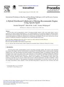
4. DHSR Approach 4.1 Approach Overview In this section, we propose a Deep Hybrid collaborative filtering approach for Service Recommendation (called DHSR), which aims to capture underlying complex interactions between mashups and services according to their invocation history and functionalities. As depicted in Fig. 1, DHSR consists of two components: a CF component and a content component. These two components are represented by respective feed-forward neural networks, whose last hidden layers are concatenated together. More specifically, the CF component decomposes the mashup-service invocation matrix, learns a latent representation of mashups and services, and models the interactions between them non-linearly and deeply. The content component firstly transforms textual descriptions of mashups and services into feature vectors that represent their content similarity by utilizing multiple similarity feature extractors and incorporating several pretrained word embeddings. Afterwards, the content component learns the latent interactions between mashups and services from the viewpoint of textual content by a neural network. Finally, to combine these two components, we concatenate their last hidden layers and then feed them into a three-layer neural network. The parameters of the whole model are trained jointly.
4.2 The CF Component In essence, the CF component learns non-linear interaction function 𝐹, latent feature matrix of mashups 𝑷 and latent feature matrix of services 𝑸, and estimates the interaction 𝑟𝑚𝑠 between mashup m and service s, as defined in Equation (1).
𝑟̂𝑚𝑠 = 𝐹(𝑚, 𝑠| 𝑷, 𝑸, 𝛩),
(1)
Sigmoid ……
ReLU ……
……
Concatenation Content Component
CF Component ……
…… …… ReLU
…… ReLU
……
……
……
ReLU
Concatenation Mashup Latent Vector
Service Latent Vector
Text Similarity Vector Extraction
0 …
Mashup-Service Invocation Matrix
0
...
0
1
0
1
...
0
...
0
0
Service (s)
Mashup Content
...
0
MxS
E E E
Service Content
Word Embeddings Mashup (m)
Fig. 1. Architecture of DHSR.
where 𝛩 denotes the parameters of 𝐹. Moreover, the traditional MF model can be deemed as a linear model of latent factors (He et al., 2017), as shown in Equation (2), 𝑟̂𝑚𝑠 = 𝒑𝒎 𝑇 𝒒𝒔 = ∑𝐾 𝑘=1 𝑝𝑚𝑘 𝑞𝑠𝑘 ,
(2)
where K denotes the dimension of the latent feature vector. In contrast, the CF component uses a multilayer perceptron (MLP) to learn the interaction function 𝐹, which is naturally non-linear. As depicted in Fig. 1, one-hot encodings of mashup 𝑚 and service 𝑠 chosen from the mashup-service invocation matrix are fed into the CF component. Details of the CF component are described as follows. The identifiers of the input mashups and services are firstly transformed into sparse binary vectors with one-hot encodings (for example, [0, 0, 1, 0, 0, 0, 0, 0, 0, 0, …, 0]), and then transformed into dense vectors, which can be viewed as latent features of mashups and services in the context of latent factor model. Towards this end, we use a fully connected layer, also known as an embedding layer, as the first hidden layer. The architecture of the embedding layer is shown in Fig. 2.
Hidden Layer Concatenation
Embedding Layer
Input Layer
0
1
0
0
0
Mashup vector
0
1
0
Service vector
Fig. 2. Substructure of the CF component. 𝑆 Two input vectors 𝒙𝑀 𝑚 and 𝒙𝑠 , represented in sparse binary vectors, denote the current mashup and service
encoded using one-hot encodings, whose sizes are 𝑀 and 𝑆, respectively. The identity function is used as the activation function in the embedding layer. 𝑻 𝑀 𝑆 𝑻 𝑆 𝑙𝑚 = 𝑓(𝒙𝑀 𝑚 |𝑷) = 𝑷 𝒙𝑚 , 𝑙𝑠 = 𝑓(𝒙𝑠 |𝑸) = 𝑸 𝒙𝑠 ,
(3)
where 𝑷 ∈ ℛ 𝑀×𝐾 , 𝑸 ∈ ℛ 𝑆×𝐾 , and 𝐾 denotes the size of the hidden layer. The embedding layer can be viewed as a lookup table, whose values are weights 𝑷 and 𝑸 of its edges. The outputs of the embedding layer are represented as: 𝑙𝑚 = [𝑝𝑚1 , 𝑝𝑚2 , … , 𝑝𝑚𝑘 ], 𝑙𝑠 = [𝑞𝑠1 , 𝑞𝑠2 , … , 𝑞𝑠𝑘 ].
(4)
Following this setting, the one-hot encodings of mashups and services are compressed into dense vectors, named as mashup embeddings and service embeddings. In this work, 𝑷 and 𝑸 are initialized with a Gaussian distribution, and are jointly learned with other parts of the neural network. Next, 𝑙𝑚 and 𝑙𝑠 are concatenated and fed into a deep neural network. More formally, the forward propagation process is defined as: 𝑙 𝑙1 = 𝑓(𝑾1𝑇 [ 𝑚 ] + 𝒃1 ), 𝑙𝑠 𝑙𝑖 = 𝑓(𝑾𝑇𝑖 𝑙𝑖−1 + 𝒃𝑖 ), 𝑖 = 2, … , 𝑁,
(5)
𝑟 𝐶𝐹 = 𝑙𝑁 , where 𝑙𝑖 (𝑖 = 1, … , 𝑁) denotes an intermediate hidden layer, 𝑾𝑖 denotes the 𝑖𝑡ℎ weight matrix, 𝒃𝑖 denotes the 𝑖𝑡ℎ bias term, 𝑟 𝐶𝐹 denotes the output of the last hidden layer of the CF component, and 𝑓 denotes the activation function. In this work, we use rectified linear unit (ReLU), which has been widely used in deep learning, as the activation function of the hidden layers: 𝑓(𝑥) = 𝑚𝑎𝑥(0, 𝑥).
(6)
4.3 The Content Component As depicted in Fig. 1, the content component with the objective of learning interactions between mashups and services in the content field consists of two parts: a similarity calculation part and a Deep Neural Network (DNN) part. Referring to the work in (Kenter & Rijke, 2015), the similarity of textual descriptions between mashups and services can be calculated by using arbitrary numbers of pre-trained word embeddings. 4.3.1 Similarity Calculation Part 𝑀 Given textual description 𝑡𝑚 of mashup m, textual description 𝑡𝑠𝑆 of service s and word embedding 𝐸, we can
extract multiple similarity features to describe semantic similarities between m and s. Three kinds of similarity feature extractors are considered. To illustrate the process of extracting similarity features, we use the example described in Section 3, in particular the similarity calculation between mashup “CoinDesk BPI” (m) and service “BitStamp HTTP” (s), as shown in Fig. 3. 𝑀 𝑆 (1) Feature extractor on the weighted semantic similarity 𝑓𝑒𝑤𝑠 ( 𝑡𝑚 , 𝑡𝑠 , 𝐸)
The weighted semantic similarity assumes that the terms in a text are not equally important, and the importance of a term can be measured by its inverse document frequency (IDF). To capture finer-grained similarity features, we set multiple intervals for the weighted semantic similarity features. Detailed process of calculating 𝑓𝑒𝑤𝑠 is described as follows. We firstly calculate the semantic similarity between each term 𝑤 in the longer text and the shorter text 𝑡 under a given word embedding 𝐸, which is defined as the maximum of cosine similarities between embedding vectors of 𝑤 and each term in 𝑡. 𝑠𝑒𝑚(𝑤, 𝑡, 𝐸) = 𝑀𝐴𝑋({𝑐𝑜𝑠𝑖𝑛𝑒𝑆𝑖𝑚(𝐸(𝑤), 𝐸(𝑤 ′ ))|𝑤 ′ ∈ 𝑡}), 𝑐𝑜𝑠𝑖𝑛𝑒𝑆𝑖𝑚(𝐸(𝑤), 𝐸(𝑤 ′ )) =
𝐸(𝑤) ∙ 𝐸(𝑤 ′ ) , ‖𝐸(𝑤)‖‖𝐸(𝑤 ′ )‖
(7) (8)
where 𝐸(𝑤) denotes the embedding vector of term 𝑤 under embedding 𝐸, and 𝑀𝐴𝑋(𝑆) denotes the maximum 𝑆 𝑀 𝑀 of set 𝑆. In other words, we calculate 𝑠𝑒𝑚(𝑤, 𝑡𝑠𝑆 , 𝐸) (or 𝑠𝑒𝑚(𝑤, 𝑡𝑚 , 𝐸), if |𝑡𝑀 𝑚 | < |𝑡𝑠 |) for each term 𝑤 in 𝑡𝑚 (or
𝑡𝑠𝑆 ). Next, we assign these values of 𝑠𝑒𝑚 to predefined intervals, and then calculate the weighted semantic similarity 𝑓𝑒𝑤𝑠 (𝑤, 𝑡, 𝐸) between 𝑤 and 𝑡.
service s
mashup m
embedding E
coindesk, bitcoin, price, index, represent, average, ...
E E
Calculate cosineSim between term vectors
Calculate sem
bitstamp bitstamp online exchange bitcoin ...
coindesk 0.5412
0.1852 0.5426 0.8845 1.0000 ...
sem
...
Assign sem values to intervals -1 ~ 0.15 0.1498, 0.1043, ...
0.15 ~ 0.40
0.40 ~ 0.80 0.80 ~ 1
0.1852, 0.2623, ...
0.5426, 0.6655, ...
0.8845, 1.0000, ...
0.9812, 0.7955, ...
2.3428, 3.1842, ...
1.7201, 4.8615, ...
Average values of each interval
...
...
...
0.2001 0.3416
index 0.1272
...
0.1476 0.1328
m 0.1416 -0.0270 -01845 0.1758 ... S 0.1751 -0.1328 0.1494 -0.0291... Calculate cosine similarity
Assign cosineSim values to intervals
0.3063, 0.2122, ...
0.80 ~ 1 4.6947, 5.9410, ...
0.5198 0.6122
...
...
-1 ~ 0.45
0.15 ~ 0.40 0.40 ~ 0.80
Transform embedding vectors
exchange bitcoin
price 0.3122
Calculate 𝑓𝑒𝑤𝑠 -1 ~ 0.15
bitstamp, ` online, exchange, bItcoin, online, consumer, ...
E
0.45 ~ 0.80 0.80 ~ 1 0.5412, 0.5198, ...
0.8123, 0.8876, ...
0.7854
Average values of each interval 0.2199
0.8762
Step 1.1: Calculate the weighted semantic similarity
0.5531
2.4001 5.0168 4.1029
0.9843 Step 1.2: Calculate the unweighted semantic similarity
Step 1.3: Calculate the mean term similarity
Step 2: Concatenate
0.8762 2.4001 5.0168 4.1029 0.2199 0.5531 0.9843 0.7854
𝑓𝑒𝑤𝑠
𝑓𝑒𝑢𝑛
𝑓𝑒𝑚𝑡 𝑠
Fig. 3. Illustration of the similarity calculation process. 𝑓𝑒𝑤𝑠 (𝑤, 𝑡, 𝐸) = 𝐼𝐷𝐹(𝑤) ∙
𝑠𝑒𝑚(𝑤, 𝑡, 𝐸) ∙ (𝑘 + 1) 𝑠𝑒𝑚(𝑤, 𝑡, 𝐸) + 𝑘 ∙ (1 − 𝑏 + 𝑏 ∙
|𝑡| ) 𝑎𝑣𝑔𝑙
,
(9)
where 𝐼𝐷𝐹(𝑤) denotes the IDF value of term 𝑤, 𝑎𝑣𝑔𝑙 denotes the average length of descriptions of all mashups and services, 𝑘 and 𝑏 are smooth parameters, and |𝑡| denotes the length of 𝑡. Finally, the values of 𝑓𝑒𝑤𝑠 (𝑤, 𝑡, 𝐸) within each interval are averaged to obtain a finer-grained similarity feature. Example. We set the intervals used in the weighted semantic similarity as: -1~0.15, 0.15~0.4, 0.4~0.8, and 0.8~∞, as described in Section 5.1. As shown in Step 1.1 of Fig. 3, since the description of service s is longer than that of mashup m, we firstly calculate semantic similarities (sem) between each term w in the description of s with the description of m according to Equation (7). The result is {0.1852, 0.5426, 0.8845, 1.0000, 0.3254,
0.2623, 0.7842, …}. Each similarity value of sem will be assigned to one of the four intervals. For example, {0.5426, 0.6655, 0.7842, ...} is assigned to interval 0.4~0.8. Afterwards, 𝑓𝑒𝑤𝑠 will be calculated according to Equation (9). Finally, the values of 𝑓𝑒𝑤𝑠 within each interval are averaged. In this way, the weighted semantic similarity vector between m and s can be represented as [0.8762, 2.4001, 5.0168, 4.1029]. 𝑀 𝑆 (2) Feature extractor on the unweighted semantic similarity 𝑓𝑒𝑢𝑛 (𝑡𝑚 , 𝑡𝑠 , 𝐸)
The unweighted semantic similarity assumes that the terms in a text are equally important. We firstly 𝑀 calculate the value of 𝑐𝑜𝑠𝑖𝑛𝑒𝑆𝑖𝑚(𝐸(𝑤), 𝐸(𝑤 ′ )) for each term pair 𝑤 ∈ 𝑡𝑚 and 𝑤 ′ ∈ 𝑡𝑠𝑆 according to Equation
(8), and then assign these values of 𝑐𝑜𝑠𝑖𝑛𝑒𝑆𝑖𝑚(𝐸(𝑤), 𝐸(𝑤 ′ )) to predefined intervals. Finally, we take the average of values within each interval to obtain a finer-grained similarity feature. Example. We set the intervals used in the unweighted semantic similarity as: -1~0.45, 0.45~0.8, and 0.8~1, as described in Section 5.1. As shown in Step 1.2 of Fig. 3, we firstly calculate the cosine similarities (cosineSim) of all term vectors between m and s. Next, each value of cosineSim will be assigned to one of the three intervals, respectively. Finally, the values within each interval are averaged, and the unweighted semantic similarity vector is [0.2199, 0.5531, 0.9843]. 𝑀 𝑆 (3) Feature extractor on the mean term similarity 𝑓𝑒𝑚𝑡𝑠 (𝑡𝑚 , 𝑡𝑠 , 𝐸) 𝑀 The mean term similarity takes the average of embedding vectors for each term in 𝑡𝑚 and 𝑡𝑠𝑆 , respectively;
and then calculates their cosine similarity. 𝐸(𝑤) 𝐸(𝑤) , ∑ ). 𝑀 𝑙𝑒𝑛( 𝑡𝑚 ) 𝑙𝑒𝑛( 𝑡𝑠𝑆 ) 𝑀 𝑆
𝑀 𝑆 𝑓𝑒𝑚𝑡𝑠 (𝑡𝑚 , 𝑡𝑠 , 𝐸) = 𝑐𝑜𝑠𝑖𝑛𝑒𝑆𝑖𝑚( ∑
𝑤 ∈ 𝑡𝑚
(10)
𝑤 ∈ 𝑡𝑠
Please note that the mean term similarity cannot be further classified into more similarity features since it takes the average of term vectors within each text in advance. Example. As shown in Step 1.3 of Fig. 3, we firstly transform the embedding vectors of m and s, and then calculate the cosine similarity between two new vectors using Equation (10). The result is 0.7854. Finally, these similarity features are concatenated to construct a new vector. Example. As shown in Step 2 of Fig. 3, we concatenate these three types of similarities and get a feature vector of length eight [0.8762, 2.4001, 5.0168, 4.1029, 0.2199, 0.5531, 0.9843, 0.7854] to represent the similarity between m and s under embedding E. Moreover, we further consider more kinds of word embeddings to construct more feature vectors of similarities, which will be finally concatenated together and fed into a deep neural network. The detailed process of calculating the similarity 𝑆𝑖𝑚𝑚,𝑠 between mashup 𝑚 and service 𝑠 is described in Algorithm 1.
Algorithm 1: Similarity Calculation for Mashups and Services 𝑀 Input: functional description 𝑡𝑚 of mashup 𝑚, functional description 𝑡𝑠𝑆 of service 𝑠, sets
of word embeddings 𝐸𝑖 (𝑖 = 1, 2, … , 𝑁) Output: similarity 𝑆𝑖𝑚𝑚,𝑠 between mashup 𝑚 and service 𝑠 1.
set 𝑆𝑖𝑚𝑚,𝑠 to empty feature vector;
2.
for 𝑖 from 1 to 𝑁 do
3.
𝑀 𝑆 calculate 𝑓𝑒𝑤𝑠 (𝑡𝑚 , 𝑡𝑠 , 𝐸𝑖 ) with multiple intervals;
4.
𝑀 𝑆 calculate 𝑓𝑒𝑢𝑛 (𝑡𝑚 , 𝑡𝑠 , 𝐸𝑖 ) with multiple intervals;
5.
𝑀 𝑆 calculate 𝑓𝑒𝑚𝑡𝑠 (𝑡𝑚 , 𝑡𝑠 , 𝐸𝑖 );
6.
𝑀 𝑆 𝑀 𝑆 𝑀 𝑆 concatenate 𝑆𝑖𝑚𝑚,𝑠 with 𝑓𝑒𝑤𝑠 (𝑡𝑚 , 𝑡𝑠 , 𝐸𝑖 ), 𝑓𝑒𝑢𝑛 (𝑡𝑚 , 𝑡𝑠 , 𝐸𝑖 ), and 𝑓𝑒𝑚𝑡𝑠 (𝑡𝑚 , 𝑡𝑠 , 𝐸𝑖 );
7.
end for
4.3.2 DNN part Once 𝑆𝑖𝑚𝑚,𝑠 is obtained from the similarity calculation part, it is fed into a deep neural network. More formally, the forward propagation process is defined as follows: 𝑙1 = 𝑓(𝑾1𝑇 𝑆𝑖𝑚𝑚,𝑠 + 𝒃1 ), 𝑙𝑖 = 𝑓(𝑾𝑇𝑖 𝑙𝑖−1 + 𝒃𝑖 ), 𝑖 = 2, … , 𝐿
(11)
𝑟 𝐶𝑜𝑛𝑡𝑒𝑛𝑡 = 𝑙𝐿 , where 𝑙𝑖 , 𝑾𝑖 , and 𝒃𝑖 (𝑖 = 1, … , 𝐿 ) denote the 𝑖𝑡ℎ intermediate hidden layer, weight matrix and bias term, respectively. Here we still use ReLU as the activation function of the hidden layers.
4.4 Combination of the two components The CF component and the content component are combined by concatenating their last hidden layers and then fed into a new hidden layer to learn the interaction between them non-linearly. We use the sigmoid function as the activation function of the output layer for implicit feedback prediction, and use ReLU as the activation function of the hidden layer. The output of the sigmoid function in the output layer, in other words, the probability of a service to be invoked by a mashup, can be seen as the result of service recommendation. The forward propagation of the whole model can be formally described as follows. 𝑷𝑇 𝒙𝑀 𝑇 𝑇 𝑟 𝐶𝐹 = 𝑓(𝑾1,𝑁 (… 𝑓 (𝑾1,1 [ 𝑇 𝑚𝑆 ] + 𝒃1,1 ) … ) + 𝒃1,𝑁 ), 𝑸 𝒙𝑠 𝑟 𝐶𝑜𝑛𝑡𝑒𝑛𝑡 = 𝑓(𝑾𝑇2,𝐿 (… 𝑓(𝑾𝑇2,1 𝑆𝑖𝑚𝑚,𝑠 + 𝒃2,1 ) … ) + 𝒃2,𝐿 ), 𝑟 𝐶𝐹 ] + 𝒃 ) + 𝒃 )), 𝑟̂𝑚𝑠 = 𝜎 (𝑾𝑇3,2 (𝑓 (𝑾𝑇3,1 [ 𝐶𝑜𝑛𝑡𝑒𝑛𝑡 3,1 3,2 𝑟
(12)
where 𝑾1,𝑖 and 𝒃1,𝑖 denote the 𝑖𝑡ℎ weight matrix and the bias term of the CF component, 𝑾2,𝑖 and 𝒃2,𝑖 denote the 𝑖𝑡ℎ weight matrix and the bias term of the content component, and 𝑾3,𝑖 and 𝒃3,𝑖 denote the 𝑖𝑡ℎ weight matrix and the bias term of the combination layer. 𝑁 and 𝐿 denote the numbers of hidden layers of the CF component and the content component, respectively. 𝑟̂𝑚𝑠 denotes the prediction of the implicit feedback.
4.5 Model learning and prediction In a recommendation model, the objective function is used to determine how the model training penalizes deviations between predicted values and the ground truth, which can significantly affect the recommendation performance. Pointwise and pairwise are two types of loss functions commonly used in recommender systems. The pointwise loss function selects a single instance each time and transforms the recommendation task into a regression or classification problem. Squared loss and log loss (He et al., 2017) are two typical loss functions of this type. The pairwise loss functions, such as Bayesian personalized ranking (BPR) (Rendle, Freudenthaler, Gantner, & Schmidt-Thieme, 2009) and AUC loss, select a pair of instances each time and transform the recommendation task into a pairwise classification problem. Both the two kinds of functions can be applied in Web service recommendation. When applying pointwise loss, we use all invocation relations between mashups and their component services as positive instances and sample negative instances from unobserved mashupservice invocation relations uniformly by controlling a negative sampling ratio (denoted as nsr). When applying pairwise loss, we pair exactly one sampled negative instance with a positive one and optimize model parameters to make the positive instance always ranked higher than the negative one. Specifically, for any mashup 𝑚 and one of its component services 𝑠 (that is, 𝑟𝑚𝑠 = 1), we uniformly sample an un-invoked service 𝑛 (that is, 𝑟𝑚𝑛 = 0) to form a triplet (𝑚, 𝑠, 𝑛). Note that predicted rating 𝑟̂𝑚𝑠 should be higher than 𝑟̂𝑚𝑛 . Algorithm 2: Training Algorithm of DHSR Input: sets of word embeddings 𝐸𝑖 (𝑖 = 1,2, … , 𝑁) , sets of similarity feature extractors 𝑓𝑒𝑖 (𝑖 = 1,2, … , 𝐿), set of mashup descriptions 𝑡 𝑀 , set of service descriptions 𝑡 𝑆 , mashupservice invocation matrix 𝑅, negative sampling ratio 𝑛𝑠𝑡, number of epochs Epochs, and batch size bts. Output: Weight matrices and bias terms 𝑷, 𝑸, 𝑾1 , 𝑾2 , 𝑾3 , 𝒃1 , 𝒃2 , 𝒃3 . 1.
initialize 𝑷, 𝑸, 𝑾1 , 𝑾2 , 𝑾3 according to Gaussian distribution;
2.
initialize 𝒃1 , 𝒃2 , 𝒃3 to 0;
3.
uniformly sample unobserved invocations as 𝑅− according to 𝑛𝑠𝑡;
4.
set 𝑅+ to all observed invocations and set 𝑅 to 𝑅 + ∪ 𝑅− ;
5.
for epoch = 1, …, Epochs do
6.
shuffle 𝑅 and partition 𝑅 into 𝑅1 , … , 𝑅𝑡 according to bts;
7.
for iter = 1, …, t do
8.
for each mashup m and service s in 𝑅𝑖𝑡𝑒𝑟 do
9.
compute 𝑙𝑚 and 𝑙𝑠 according to Equation (3);
10.
compute 𝑟 𝐶𝐹 according to Equation (5);
11.
compute 𝑆𝑖𝑚𝑚,𝑠 using Algorithm 1;
12.
compute 𝑟̂𝑚𝑠 according to Equation (12);
13.
end for
14.
optimize model parameters using Adam;
15.
end for
16. end for
The pointwise loss can flexibly set the sampling ratio of negative instances, while the pairwise loss can only pair a negative instance with a positive one. Therefore, pointwise is better than pairwise in some recommendation scenarios (He et al., 2017), particularly in the service recommendation field where the number of services used by each mashup is very small, and the interaction matrix is thus extremely sparse. According to this consideration, we use log loss, which is the binary cross-entropy, as the loss function of our model. Moreover, we use 𝐿2 regularization to prevent model overfitting. The cost function 𝐽 to be minimized is defined as follows. 𝐽=−
∑
𝑟𝑚𝑠 𝑙𝑜𝑔 𝑟̂𝑚𝑠 + (1 − 𝑟𝑚𝑠 ) 𝑙𝑜𝑔(1 − 𝑟̂𝑚𝑠 ) +
(𝑚,𝑠)∈𝑅+ ∪𝑅−
𝜆 ∥ 𝛩 ∥22 , 2
(13)
where 𝑅+ denotes the set of positive instances, 𝑅 − denotes the set of negative instances, 𝜆 is the regularization parameters, and 𝛩 is the weights of edges. We use the mini-batch Adaptive Moment Estimation (Adam) (Kingma & Ba, 2014) to learn our proposed model. The total training process of DHSR is described in Algorithm 2. The derivative of the model can be calculated with back-propagation, which are omitted in this paper. Once the model is learned, we can conduct model prediction according to user requests in mashup development. For a given request of mashup 𝑚, the recommendation procedure can be described as follows. We firstly calculate the score between 𝑚 and each candidate service 𝑠 in the training set according to Equation (12), which represents the probability of 𝑠 being recommended to 𝑚. Afterwards, all the scores are sorted and the top N services are finally recommended for the development of mashup 𝑚. We still use the example in Section 3 to illustrate the training and recommendation processes. Because the major steps of the two processes are very similar except that the training process includes a step of model
parameter optimization, we only show how the model can recommend services for a given mashup (e.g., “CoinDesk BPI”, denoted as m). At this stage, the scores between “CoinDesk BPI” and all services in the registry should be calculated by DHSR, and N services with the top scores will be selected as the recommendation result. We use the calculation process between service “BitStamp HTTP” (s) and the mashup m for illustration, as shown in Fig. 4. mashup m
service s
mashup m 0 0 1 0 0 0 0 0 0 0 ... 0
0 0 0 0 0 0 1 0 0 0 ... 0 Transform latent vector
Transform latent vector 1.26e-16 -1.18e-24 -2.78e-24 ...
mashup latent vector Step 1.1: obtain the score vector of the CF component
service s
E
bitstamp, online, exchange, bItcoin, online, consumer, ...
E E Calculate similarity vector
-0.2098 -0.2515 -0.1788 ...
0.8762 2.4001 5.0168 4.1029 0.2199 0.5531 0.9843 0.7854 ...
Concatenate 1.26e-16 -1.18e-24 -2.78e-24 ...
embedding E
coindesk, bitcoin, price, index, represent, average, ...
Calculate 𝑟 𝐶𝑜𝑛𝑡𝑒𝑛𝑡
-0.2098 -0.2515 -0.1788 ...
0.8649 1.1665 1.4680 0.8577 ...
service latent vector
Calculate 𝑟 𝐶𝐹
Step 1.2: obtain the score vector of the content component
0.0185 0.1489 0.1678 0.1311 ...
Concatenate 0.0185 0.1489 0.1678 0.1311 ...
0.8649 1.1665 1.4680 0.8577 ...
𝑟 𝐶𝐹
𝑟 𝐶𝑜𝑛𝑡𝑒𝑛𝑡 Calculate 𝑟̂𝑚𝑠
Step 2: Concatenate and predict
0.8640
Fig. 4. Illustration of the DHSR-based service recommendation process.
Step 1: The first step is to obtain the score vectors of the CF component and the content component, which are detailed in the following two sub-steps, respectively. Step 1.1: In the CF component, the one-hot encodings of m and s: [0, 0, 1, 0, 0, 0, 0, 0, 0, 0, …, 0] and [0, 0, 0, 0, 0, 0, 1, 0, 0, 0, …, 0], are firstly transformed into dense latent vectors: [-1.2563e-16, -1.1837e-24, -2.7764e24, -1.4276e-24, -2.5638e-15, -2.9917e-15, -5.1344e-25, 1.0564e-35] and [-0.2098, -0.2515, -0.1788, -0.2060, 0.2366, 0.2042, -0.2030, -0.1895], respectively. Afterwards, the two vectors are concatenated and their concatenation is then fed into an MLP to obtain the score vector 𝑟 𝐶𝐹 of the CF component using Equation (5). The result of 𝑟 𝐶𝐹 is: [0.0185, 0.1489, 0.1678, 0.1311, 0.1703, 0, 0.1771, 0.0331, 0, 0.1794, 0.0348, 0.1880, 0, 0.2106, 0, 0]. Step 1.2: In the content component, the similarities between their textual descriptions are firstly calculated and concatenated, resulting in a similarity feature vector: [0.8762, 2.4001, 5.0168, 4.1029, 0.2199, 0.5531, 0.9843, 0.7854, 0, 2.6780, 3.9239, 4.9650, 0.2561, 0.5683, 0.9271, 0.7136, 0, 2.4982, 5.0871, 4.2298, 0.2255, 0.5714, 0.9731, 0.7412]. Afterwards, the similarity feature vector is fed into an MLP to obtain the score vector
𝑟 𝐶𝑜𝑛𝑡𝑒𝑛𝑡 of the content component using Equation (11). The result of 𝑟 𝐶𝑜𝑛𝑡𝑒𝑛𝑡 is: [0.8649, 1.1665, 1.4680, 0.8577, 0.5067, 0.0135, 0.4424, 0.0464, 0.1132, 0.6547, 1.0098, 0.4218]. Step 2: Two score vectors 𝑟 𝐶𝐹 and 𝑟 𝐶𝑜𝑛𝑡𝑒𝑛𝑡 are concatenated and fed into an MLP to calculate 𝑟̂𝑚𝑠 using Equation (12). 𝑟̂𝑚𝑠 denotes the predicted probability of service s to be invoked by mashup m. The result of 𝑟̂𝑚𝑠 in this example is 0.8640. Step 3: Similarly, we can predict a list of similarity scores between the mashup m and all other services in the service registry, e.g., {0.8640, 0.0293, 0.1073, 0.0856, 0.1423, 0.0260, 0.3434, 0.1151, 0.8566, …}, and finally the services with top scores can be recommended for m. Please note that this step is not shown in Fig. 4 since Fig.4 only illustrates the calculation process of a mashup with a service.
4.6 Computational Complexity Analysis We further analyze the computational complexity of the proposed approach. For each epoch, the similarity calculation of the content component costs about O(𝑎𝑣𝑔𝑠𝑙 ∗ 𝑎𝑣𝑔𝑚𝑙 ∗ 𝐸 ∗ (𝑛𝑠𝑡 + 1) ∗ 𝐼), where 𝑎𝑣𝑔𝑠𝑙 is the average length of the service description, 𝑎𝑣𝑔𝑚𝑙 is the average length of the mashup description, 𝐸 is the number of word embeddings, 𝑛𝑠𝑡 is the negative sampling ratio, and 𝐼 is the number of observed ratings. Among these parameters, 𝑎𝑣𝑔𝑠𝑙 and 𝑎𝑣𝑔𝑚𝑙 are close to a constant. In the data set we used in experiments, the average lengths of services and mashups are 42.91 and 22.87, respectively. 𝐸 is set to 3 in our experiments, which can also be viewed as a constant if the experimental setting is fixed. 𝑛𝑠𝑡 is another constant during experiment setting. Therefore, the cost of the similarity calculation is approximately linear to the number of observed ratings in the interaction matrix. Note that the complexity listed here is the maximum possible value because the calculated similarities can be cached for calculation in subsequent epochs. Referring to the complexity analysis of the neural network (Kim, Park, Oh, Lee, & Yu, 2016), the computational complexity of the neural network part of our model can be seen as scaling linearly with the size of given data when all parameters, such as the number of layers and the number of neurons, are fixed. Therefore, if experimental parameters of the neural network are fixed, the computation time of the entire optimization process of DHSR grows approximately linearly with respect to the size of given data. The complexity analysis shows that our proposed approach can be applied in large-scale systems.
5 Experiments In this section, we conducted a series of experiments to evaluate the proposed DHSR based on a real-world Web service dataset. These experiments were designed to answer the following three research questions:
RQ1: Does the proposed DHSR outperform the state-of-the-art Web service recommendation methods?
RQ2: Which kind of objective functions, pairwise loss or pointwise loss, is better for the service recommendation task?
RQ3: Will the recommendation result be affected by adding the number of word embeddings?
5.1 Experimental settings We conducted a series of experiments to evaluate our proposed approach. All the experiment programs were developed in Python, and carried out on a PC with Intel Core 4 CPU i7-4710HQ, @2.5 GHz and 8 GB RAM, running the Windows 10 OS. 5.1.1 Dataset Table 1. Example of mashups and services in the dataset. (a) Mashup “CoinDesk Bitcoin Price Index (BPI)”
Attribute Mashup name Category Component services Description
Value CoinDesk Bitcoin Price Index (BPI) Bitcoin, Currency, Prices Mt Gox, BitStamp HTTP, BTC-e, Bitfinex “The CoinDesk Bitcoin Price Index (BPI) represents an average of bitcoin prices across leading global exchanges that meet criteria specified by the BPI. …” (b) Service “BitStamp HTTP”
Attribute Name Category Description
Value BitStamp HTTP Financial, Currency, Marketplace “BitStamp is an online exchange for bitcoins. Online consumers and traders can use it as a global marketplace to buy and sell BitCoins. …” Table 2. Statistics of the dataset.
Statistics Number of services Number of mashups Average number of services in mashups Number of mashup-service interaction Vocabulary size Average number of word tokens in services Average number of word tokens in mashups Average number of categories of mashups and services
Value 13,520 5,769 1.90 10,950 27,831 42.91 22.87 3.39
Statistics of the dataset. ProgrammableWeb (PW) is by far the largest online Web service and mashup registry. To evaluate the performance of the proposed DHSR, we crawled a dataset from PW on July 25, 2016. The dataset consists of 13,520 services and 5,769 mashups. Because we are only interested in the services
invoked by at least one mashup, and many services have been deprecated, the dataset was thus reduced to containing 5,769 mashups and 1,103 services. The sparsity of the interaction matrix in the dataset is about 99.83%. The dataset contains descriptions and tags (including the primary and secondary categories) of mashups and services and the invocation relations between them. For example, Table 1 shows a mashup and a service in the dataset, where service “BitStamp HTTP” is a component service of mashup “CoinDesk Bitcoin Price Index (BPI).” Table 2 illustrates the detailed statistial information of the dataset. Dataset preparation. In our dataset, the functionalities of mashups and services are embodied in their textual descriptions and tags (also knowns as categories). Considering that the tags are manually added by the PW administrators and are thus more valuable in identifying services or mashups, we used amplification coefficient α to amplify the weights of tags and combined them with textual descriptions to construct a functional description corpus. Afterwards, we performed the following steps to preprocess the extracted corpus. Spelling correction. We leveraged PyEnchant2, an English spell checking library for Python, to replace misspelled words. Tokenization. The NLTK3 toolkit was used to obtain lists of words (also known as tokens) from the input corpus. Stopword removal. The built-in stopword list in the NLTK toolkit was utilized to remove the common words frequently occurred in written English. Lemmatization. We used the WordNet4 Lemmatizer packaged in the NLTK toolkit to reduce all words to their root forms. After preprocessing the dataset, we further prepared the word embeddings for subsequent calculation. We used two kinds of word embeddings. The first is the publicly released word embeddings, referred to as reference embeddings. The reference embeddings we used are described as follows. The word embedding generated in (Baroni, Dinu, & Kruszewski, 2014) consists of vectors with 400-dimensional, 5-word context window, and 10 negative samples; and the Glove word embedding (Pennington, Socher, & Manning, 2014) consists of 840 billion tokens, 2.2 million vocabularies, and 300-dimensional vectors. To deal with out-of-vocabulary words, we adopted two strategies. The first strategy is dividing the compound words and summing their embedding vectors. For example, compound word “crypto-currency” can be transformed into the sum of 𝐸("crypto") and 2
https://pythonhosted.org/pyenchant/
3
http://www.nltk.org/
4
http://wordnet.princeton.edu/
𝐸("currency"). The intuition behind this strategy is that the distributional semantic approach such as Word2vec, can capture the deep-level semantic information and subtle semantic relationships between words (Mikolov, Chen, Corrado, & Dean, 2013). The second strategy is to map terms to random vectors, which is widely applied in text mining. Moreover, we trained a word embedding on the service corpus on our own, referred to as the local embedding. We used Word2vec to train the local embedding, and adopted Skip-gram as the architecture and hierarchical softmax as the optimization model. The window width and the vector dimensionality were set to 5 and 80, respectively. Training set and test set. To evaluate the recommendation performance, we constructed a training set and a test set for each experiment based on the crawled dataset. Firstly, we randomly selected 30% of the mashups that include more than one component service as the test set, and the rest mashups were used as the training set. Note that we randomly selected 10% of the training set as the validation set. Then, for each mashup in the test set, one service was randomly selected from the component services of the mashup. The selected services were included in mashup requirements (namely they acted as a part of user input) while the remaining services of each mashup in the test set were used for prediction. Each experiment was performed 20 times, and their average values were taken as reported results. 5.1.2 Evaluation Metrics In the experiments, we adopted five metrics to evaluate the recommendation performance of DHSR. Mean Average Precision (MAP) at top N services in the ranking list is defined as: MAP@𝑁 =
𝑁 1 1 𝑁𝑖 ∑ ∑ ( ∙ 𝐼(𝑖)) , |𝑀| 𝑁𝑚 𝑖=1 𝑖
(14)
𝑚∈𝑀
where 𝑁𝑚 is the number of component services of mashup 𝑚, 𝑁𝑖 denotes the number of component services of 𝑚 occurred in the top 𝑖 services of the ranking list, 𝑀 is the mashups in the test set, and 𝐼(𝑖) indicates whether the service at ranking position 𝑖 is a component service of 𝑚. Normalized Discounted Cumulative Gain (NDCG) at top N services in the ranking list is defined as: NDCG@𝑁 =
𝑁 1 1 2𝐼(𝑖) − 1 ∑ ∑ , |𝑀| 𝑆𝑚 𝑖=1 𝑙𝑜𝑔2 (1 + 𝑖)
(15)
𝑚∈𝑀
where 𝑆𝑚 represents the ideal maximum DCG score that can be achieved for 𝑚. Precision, Recall and F1-measure at top N services in the ranking list are defined as: Precision@𝑁 =
|𝑟𝑒𝑐(𝑚) ∩ 𝑡𝑟𝑢𝑡ℎ(𝑚)| 1 ∑ , |𝑀| |𝑟𝑒𝑐(𝑚)| 𝑚∈𝑀
(16)
|𝑟𝑒𝑐(𝑚) ∩ 𝑡𝑟𝑢𝑡ℎ(𝑚)| 1 ∑ , |𝑀| |𝑡𝑟𝑢𝑡ℎ(𝑚)|
(17)
|𝑟𝑒𝑐(𝑚) ∩ 𝑡𝑟𝑢𝑡ℎ(𝑚)| 1 ∑2 , |𝑀| |𝑟𝑒𝑐(𝑚)| + |𝑡𝑟𝑢𝑡ℎ(𝑚)|
(18)
Recall@𝑁 =
𝑚∈𝑀
F1@𝑁 =
𝑚∈𝑀
where 𝑟𝑒𝑐(𝑚) is a recommended service list for mashup 𝑚 , and 𝑡𝑟𝑢𝑡ℎ(𝑚) is a set of services that have interactions with 𝑚 in the test set (namely the actual component services of 𝑚). 5.1.3 Competing approaches We chose several state-of-the-art recommendation algorithms for comparison. Considering that our approach incorporates textual information and collaborative filtering (CF), these selected algorithms cover CF method, matrix factorization method, content-based method, and hybrid method, to make a comprehensive comparison.
CF (Xu et al., 2013). CF is a classical recommendation technique that has been widely used in many recommendation systems. We implemented user-based CF in our experiment.
SVD (Paterek, 2007). SVD is a classical matrix factorization technique used in recommender systems.
BPR-kNN (Rendle et al., 2009). BPR-kNN uses BPR to learn service recommendation models from the implicit feedback of mashups with a pairwise ranking loss.
NCF (He et al., 2017). Neural Collaborative Filtering (NCF) is adopted to capture the non-linear relationship between mashups and services and recommend relevant services.
TF-IDF (Xia et al., 2015). Services are recommended according to TF-IDF based cosine similarities with mashup requests.
PaSRec (Liang et al., 2016). PaSRec learns a CF based service recommendation model with implicit feedback of mashup using BPR.
5.1.4 Parameter Settings We implemented our proposed approach based on Keras5, a widely adopted deep learning library. To ensure that the hyper-parameters of DHSR can obtain the best recommendation result, we randomly sampled an interaction for each mashup to construct a cross-validation set and tuned the hyper-parameters accordingly. The model parameters were randomly initialized by following a Gaussian distribution with a mean of 0 and standard deviation of 0.01. According to the result of parameter tuning, the batch size, the learning rate, and the number of latent factors was set to 8, 0.001, and 8, respectively. Similar to most neural networks, the architecture of our
5
https://keras.io/
network model is designed by following the tower pattern, where each upper layer has a smaller number of neurons than its lower layer. Because the size of PW dataset is relatively small, setting too many hidden layers will result in overfitting, and thereby reduce the performance of service recommendation. We set the layer number of the CF component to 4 (including the embedding layer), the layer number of the content component to 3, and regularization parameter λ to 0.01, respectively. In our experiments, we set amplification coefficient α to 2. In the similarity calculation part of the content component, we also tuned parameters to achieve optimized results. k and b were set to 1.2 and 0.75, respectively. The intervals used in the weighted semantic similarity were set to -1~0.15, 0.15~0.4, 0.4~0.8, and 0.8~∞, while the intervals used in the unweighted one were set to -1~0.45, 0.45~0.8, and 0.8~1.
5.2 Performance Comparison (RQ1) Fig. 5 shows the performance of different approaches on five evaluation metrics. As can be seen, our approach exhibits improvements over all competing methods across all ranking positions, and we further conducted paired t-tests according to the repetitive experimental results, verifying that all improvements are statistically significant. More specifically, the improvements compared with PaSRec are significant at the 0.05 level (namely p < 0.05), while the improvements compared with other five approaches are significant at the 0.01 level (namely p < 0.01). Among the four CF based approaches (CF, SVD, BPR-kNN, and NCF), NCF performs the best on all evaluation metrics. The limitations of CF, BPR-kNN, and SVD lie in that they cannot accurately characterize the interactions between mashups and services due to the high sparsity of the interaction matrix. While NCF adopts a neural network architecture to capture non-linear relations between mashups and services, which can more accurately discover their relations and thus obtain relatively better performance.
(a) MAP@N
(b) NDCG@N
(c) Precision@N
(d) Recall@N
(e) F1@N
Fig. 5. Performance comparisons of different approaches on the test set.
As a content-based approach, TF-IDF characterizes the similarities between textual contents of mashups and services and then recommends similar services for mashups. Experiments show that TF-IDF performs better than CF, SVD, and BPR-kNN. The results indicate that textual contents of mashups and services can provide substantial support for service recommendation, which also validates our hypothesis of incorporating textual contents in service recommendation. Moreover, PaSRec, a latest service recommendation method, is better than the above methods on all metrics. In essence, this approach is a hybrid approach by integrating contents with CF, which fully exploits the heterogeneous information network composed of mashups and services as well as implicit feedbacks. The advantage of PaSRec demonstrates the effectiveness of the hybrid recommendation method in service recommendation. Even though PaSRec leverages more comprehensive information such as providers of services and mashups, our model DHSR still achieves better performances. Moreover, compared with NCF, a latest deep learning based recommendation method, DHSR increases by 8.62%, 9.67%, 1.93%, 11.85%, and 3.10%, on MAP@10, NDCG@10, Precision@10, Recall@10, and F1@10, respectively, which further validates our hypothesis of incorporating textual content. 5.2.1 Impact of K DHSR decomposes the mashup-service invocation matrix into two K-dimensional latent vectors. The setting of K is a key issue in the model. If K is too large, it may cause overfitting and thus reduce the generalization ability of the model. However, if it is too small, the model may be hard to characterize interactions between mashups and services. To study the effect of K on the recommendation performance, we adjusted K from 4 to 16 with a step size 4, while fixing the other parameters. As shown in Fig. 6, when K increases from 4 to 8, values of the metrics are increasing accordingly; but when K continually increases, the recommendation performance is reduced, which suggests that the model has already been overfitting. Therefore, K=8 is the optimal setting for our experiments.
(a) MAP@N
(c) Precision@N
(b) NDCG@N
(d) Recall@N
(e) F1@N
Fig. 6. Recommendation performance under different K.
5.2.2 Impact of the percentage of training data We further compared DHSR with other baseline methods with respect to different percentages of training data. Specifically, we randomly chose 80% of the data as the training set (varied from 20% to 80% with a step size 10%) and kept the remaining 20% for testing in each round. Fig. 7 shows the results of the experiment. It is obvious that DHSR outperforms other methods on five metrics with any percentage of the training data. It can also be found that as the percentage of training data increases, DHSR achieves an improvement on the recommendation performance. Furthermore, DHSR and NCF are less sensitive to the sparsity of the training data compared to PasRec and CF, which can be explained by the fact that the non-linear nature of DHSR and NCF can alleviate the sparsity issue of the training data. Not that TF-IDF is not used for comparison in Fig. 7 because it only calculates the test data and does not depend on the training data.
(a) MAP@5
(b) MAP@10
(c) MAP@15
(d) NDCG@5
(e) NDCG@10
(g) Precision@5
(h) Precision@10
(j) Recall@5
(k) Recall@10
(m) F1@5
(f) NDCG@15
(i) Precision@15
(l) Recall@15
(n) F1@10
(o) F1@15
Fig. 7. Performance comparisons on different percentages of training data.
5.3 Pointwise vs. Pairwise (RQ2) Table 3. Evaluation results of four kinds of loss functions.
N=5
N = 10
N = 15
N = 20
N = 25
N = 30
N = 35
N = 40
N = 45
N = 50
Squared Loss
0.3421
0.3636
0.3698
0.3727
0.3747
0.3758
0.3769
0.3777
0.3785
0.3788
Log Loss
0.3411
0.3644
0.3706
0.3739
0.3755
0.3768
0.3779
0.3787
0.3792
0.3796
BPR
0.2944
0.3156
0.3227
0.3267
0.3288
0.3305
0.3314
0.3322
0.3327
0.3333
AUC Loss
0.3134
0.3356
0.3434
0.3468
0.3489
0.3505
0.352
0.3530
0.3537
0.3542
MAP
NDCG
Squared Loss
0.4101
0.4529
0.4691
0.4787
0.4860
0.4906
0.4948
0.4988
0.5028
0.5044
Log Loss
0.4117
0.4553
0.4720
0.4821
0.4877
0.4927
0.4978
0.5013
0.5034
0.5058
BPR
0.3613
0.4048
0.4247
0.4376
0.4458
0.4530
0.4571
0.4607
0.4635
0.4667
AUC Loss
0.3822
0.4268
0.4473
0.4583
0.4660
0.4727
0.4791
0.4836
0.4868
0.4896
Squared Loss
0.1674
0.1054
0.0774
0.0614
0.0517
0.0444
0.0393
0.0354
0.0326
0.0297
Log Loss
0.1720
0.1083
0.0796
0.0637
0.0528
0.0455
0.0405
0.0364
0.0329
0.0301
BPR
0.1520
0.0985
0.0740
0.0607
0.0511
0.0447
0.0396
0.0325
0.0324
0.0298
AUC Loss
0.1660
0.1051
0.0769
0.0617
0.0517
0.0446
0.0394
0.0355
0.0324
0.0296
Squared Loss
0.4980
0.6106
0.6615
0.6954
0.7219
0.7399
0.7568
0.7742
0.7904
0.7972
Log Loss
0.5067
0.6183
0.6694
0.7081
0.7337
0.7521
0.7663
0.7790
0.7913
0.8014
BPR
0.4577
0.5705
0.6345
0.6786
0.7102
0.7392
0.7551
0.7697
0.7817
0.7970
AUC Loss
0.4744
0.5908
0.6557
0.6953
0.7243
0.7517
0.7773
0.7697
0.8102
0.8235
Squared Loss
0.2295
0.1681
0.1312
0.1077
0.0925
0.0808
0.0723
0.0656
0.0608
0.0558
Log Loss
0.2340
0.1714
0.1342
0.1111
0.0943
0.0825
0.0742
0.0672
0.0613
0.0565
BPR
0.2091
0.1572
0.1254
0.1062
0.0916
0.0812
0.0727
0.0660
0.0604
0.0560
AUC Loss
0.2271
0.1675
0.1303
0.1081
0.0926
0.0811
0.0724
0.0657
0.0604
0.0555
Precision
Recall
F1
As mentioned in Section 4.5, two kinds of objective functions, pointwise loss, and pairwise loss can be used in model learning. We explored the effectiveness of these objective functions in service recommendation. In our experiments, pointwise loss functions randomly selected five non-existent interactions as negative instances for each positive instance, while pairwise loss functions paired exactly one sampled negative instance with a positive one. Three kinds of loss functions other than Log Loss were selected for comparison.
Squared Loss is a widely used pointwise loss function in model parameter learning (Hu, Koren, & Volinsky, 2008), which is based on the assumption that observations are generated from a Gaussian distribution.
Bayesian Personalized Ranking (BPR) (Rendle et al., 2009) is a pairwise loss function which is widely utilized in feedback recommendation to learn model parameters. It has shown a superior performance in Web service recommendation (Liang et al., 2016).
AUC Loss, also known as the pairwise-ranking loss and margin ranking loss (Grangier & Bengio, 2008), is a widely used pairwise loss function. Table 3 shows the effect of different loss functions on service recommendation performance. It can be found
that, in most cases, the performance of pointwise loss functions is better than that of pairwise loss functions.
This finding can be explained by that the pointwise method can flexibly set the sampling ratio of negative instances, especially in our experiments, where the interaction matrix of mashups and services is extremely sparse. In addition, different Loss functions of the same type also exhibit slight differences in recommendation performance. As can be seen from Table 3, Log Loss performs better than Squared Loss on all metrics, which also proves the effectiveness of transforming implicit feedback based service recommendation into a binary classification problem.
5.4 Will more word embeddings be helpful? (RQ3)
(a) MAP@N
(c) Precision@N
(b) NDCG@N
(d) Recall@N
(e) F1@N
Fig. 8. Performance comparisons on different number of word embeddings.
The content component of DHSR aims to extract the functional similarities between mashups and services by leveraging a variety of pre-trained word embeddings. We investigated whether more word embeddings will be helpful in the recommendation performance. Towards this end, we used three different word embeddings and made a combination of them as the input to our model, while keeping other conditions unchanged. We use “Loc” to denote the method of only using the local Word2vec embedding, “Loc + Ref-w2v” to denote using “Loc” and a reference Word2vec embedding, and “Loc + Ref-w2v + Ref-Glv” to denote using a glove reference word embedding and “Loc + Ref-w2v.” As shown in Fig. 8, with the increase of the number of word embeddings, the recommendation performance is gradually improved. We attribute this encouraging result to the fact that more different kinds of word
embeddings introduce more external semantic information, which can help DHSR explore the relations between mashups and services from more viewpoints.
5.5 Discussions and limitation analysis To sum up, in the experiments, we adopted five evaluation metrics to evaluate the recommendation performance of our proposed DHSR approach. In the first group of experiments, we showed that DHSR outperforms six state-of-the-art recommendation algorithms across all ranking positions. We further analyzed the impact of K, namely the dimension number in matrix decomposition, on the recommendation performance, and found that K=8 is the optimal setting for our experiments. We also compared DHSR with other baseline methods with respect to different percentages of training data and found that DHSR outperforms other methods with any percentage of training data. In the second group of experiments, we compared pointwise loss functions and pairwise loss functions and found that pointwise loss methods have advantages over pairwise loss methods. Finally, we investigated whether more word embeddings will be helpful in the recommendation performance, and found that more word embeddings do improve the recommendation performance since they introduce more external semantic information. There are still some limitations in the proposed approach. Currently we mainly test the proposed method for the non-incremental situation. We have not tested the case when new data is coming. Faced with the new data, different measures will be taken depending on the volume of these data. If the volume of the new data is small, we will keep the embeddings of the trained data, and only train embeddings on the new data. The weights and other parameters of the neural network can also be maintained because it is calculated on the basis of large amounts of data, which can also be applied to the new small data. If the volume of the new data is huge, the embeddings and parameters of the neural network need to be retrained. Even in this case the original text similarity calculation part can continue to be maintained, which can decrease the computation time. Determining the threshold of the volume of coming data and which measure to take depends on the tradeoff analysis between the algorithm efficiency and the recommendation performance. We still need to investigate this point further. Another limitation of our approach is that it is based on matrix factorization, which focuses more on the global information of the matrix and is not sensitive to the local information. In addition, cold start and gray sheep problems are two inherent shortcomings of CF. Wei, He, Chen, Zhou, and Tang (2017) integrated textual content features into the prediction of ratings for cold start items. Ghazanfar and Prügel-Bennett (2014) demonstrated that content-based profile of gray-sheep users could make accurate recommendations. Similarly, we enrich DHSR with textual content, which can be used to alleviate these problems to some extent. However,
textual content is only one kind of auxiliary information. There is still much other heterogeneous information of services and mashups that can be used, such as the domains and providers of mashups and users, as mentioned in (Liang et al., 2016). To find better solutions to these two problems, it is necessary to seamlessly integrate these different kinds of heterogeneous information into our model in the future.
6. Conclusion and Future Work In this paper, we proposed a deep hybrid collaborative filtering approach for service recommendation (DHSR), which can capture the complex invocation relations between mashups and services in Web service recommendation by using a multilayer perceptron. Considering that the textual content including descriptions and tags of services and mashups is also crucial in recommending services, DHSR further integrated collaborative filtering with textual content within a deep neural network. We adopted three kinds of similarity feature extractors to describe semantic similarities between mashups and services and computed the similarities of their textual descriptions by using a variety of pre-trained word embeddings. Experiments conducted on a real-world dataset demonstrated that our approach can achieve a significant improvement compared with several state-of-the-art service recommendation methods. In the future, we plan to improve our proposed approach by solving the limitations proposed in Section 5.5. Firstly, we will investigate the strategy of dealing with new data. Secondly, we will integrate more heterogeneous information of mashups and services to improve our model.
Acknowledgement This work was supported by the National Basic Research Program of China under Grant No. 2014CB340404, the National Key Research and Development Program of China under Grant No. 2017YFB1400602, the National Natural Science Foundation of China under Grant Nos. 61672387 and 61572371, the Wuhan Yellow Crane Talents Program for Modern Services Industry, and the Natural Science Foundation of Hubei Province of China under Grant No. 2018CFB511. Jian Wang is the corresponding author of this paper.
References Bai, B., Fan, Y., Tan, W., & Zhang, J. (2017). DLTSR: A Deep Learning Framework for Recommendation of Long-tail Web Services. IEEE Transactions on Services Computing, in press. doi:10.1109/TSC.2017.2681666 Baroni, M., Dinu, G., & Kruszewski, G. (2014). Don't count, predict! A systematic comparison of contextcounting vs. context-predicting semantic vectors. In Proceedings of the 52nd Annual Meeting of the Association for Computational Linguistics (pp. 238-247).
Cao, B., Liu, J., Tang, M., Zheng, Z., & Wang, G. (2013). Mashup Service Recommendation Based on User Interest and Social Network. In Proceedings of the 2013 IEEE 20th International Conference on Web Services (pp. 99-106). Chen, W., Paik, I., & Hung, P. C. K. (2015). Constructing a Global Social Service Network for Better Quality of Web Service Discovery. IEEE Transactions on Services Computing, 8(2), 284-298. doi:10.1109/TSC.2013.20 Cheng, H.-T., Koc, L., Harmsen, J., Shaked, T., Chandra, T., Aradhye, H., et al. (2016). Wide & Deep Learning for Recommender Systems. In Proceedings of the 1st Workshop on Deep Learning for Recommender Systems (pp. 7-10). Gao, W., Chen, L., Wu, J., & Bouguettaya, A. (2016). Joint Modeling Users, Services, Mashups, and Topics for Service Recommendation. In Proceedings of the 2016 IEEE International Conference on Web Services (ICWS) (pp. 260-267). Ghazanfar, M. A., & Prügel-Bennett, A. (2014). Leveraging clustering approaches to solve the gray-sheep users problem in recommender systems. Expert Systems with Applications, 41(7), 3261-3275. doi:https://doi.org/10.1016/j.eswa.2013.11.010 Grangier, D., & Bengio, S. (2008). A Discriminative Kernel-Based Approach to Rank Images from Text Queries. IEEE Transactions on Pattern Analysis and Machine Intelligence, 30(8), 1371-1384. doi:10.1109/TPAMI.2007.70791 Guo, H., Tang, R., Ye, Y., Li, Z., & He, X. (2017). DeepFM: A Factorization-Machine based Neural Network for CTR Prediction. ArXiv e-prints, 1703. Accessed March 1, 2017. http://adsabs.harvard.edu/abs/2017arXiv170304247G He, X., Liao, L., Zhang, H., Nie, L., Hu, X., & Chua, T.-S. (2017). Neural Collaborative Filtering. In Proceedings of the 26th International Conference on World Wide Web (pp. 173-182). Hu, Y., Koren, Y., & Volinsky, C. (2008). Collaborative Filtering for Implicit Feedback Datasets. In Proceedings of the 2008 Eighth IEEE International Conference on Data Mining (pp. 263-272). Jain, A., Liu, X., & Yu, Q. (2015). Aggregating Functionality, Use History, and Popularity of APIs to Recommend Mashup Creation. In Proceedings of the 13th International Conference on Service-Oriented Computing (pp. 188-202). https://doi.org/10.1007/978-3-662-48616-0_12 Kenter, T., & Rijke, M. d. (2015). Short Text Similarity with Word Embeddings. In Proceedings of the 24th ACM International on Conference on Information and Knowledge Management (pp. 1411-1420). Kim, D., Park, C., Oh, J., Lee, S., & Yu, H. (2016). Convolutional Matrix Factorization for Document ContextAware Recommendation. In Proceedings of the Proceedings of the 10th ACM Conference on Recommender Systems (pp. 233-240). Kingma, D. P., & Ba, J. (2014). Adam: A Method for Stochastic Optimization. ArXiv e-prints, 1412. Accessed December 1, 2014. http://adsabs.harvard.edu/abs/2014arXiv1412.6980K Liang, T., Chen, L., Wu, J., Dong, H., & Bouguettaya, A. (2016). Meta-Path Based Service Recommendation in Heterogeneous Information Networks. In Proceedings of the 14th International Conference on ServiceOriented Computing (pp. 371-386). https://doi.org/10.1007/978-3-319-46295-0_23 Liu, J., Tang, M., Zheng, Z., Liu, X., & Lyu, S. (2016). Location-Aware and Personalized Collaborative Filtering for Web Service Recommendation. IEEE Transactions on Services Computing, 9(5), 686-699. doi:10.1109/TSC.2015.2433251 Meng, S., Dou, W., Zhang, X., & Chen, J. (2014). KASR: A Keyword-Aware Service Recommendation Method on MapReduce for Big Data Applications. IEEE Transactions on Parallel and Distributed Systems, 25(12), 3221-3231. doi:10.1109/TPDS.2013.2297117 Mikolov, T., Chen, K., Corrado, G., & Dean, J. (2013). Efficient Estimation of Word Representations in Vector Space. ArXiv e-prints, 1301. Accessed January 1, 2013. http://adsabs.harvard.edu/abs/2013arXiv1301.3781M Paliwal, A. V., Shafiq, B., Vaidya, J., Xiong, H., & Adam, N. (2012). Semantics-Based Automated Service Discovery. IEEE Transactions on Services Computing, 5(2), 260-275. doi:10.1109/TSC.2011.19 Paradarami, T. K., Bastian, N. D., & Wightman, J. L. (2017). A hybrid recommender system using artificial neural networks. Expert Systems with Applications, 83, 300-313. doi:https://doi.org/10.1016/j.eswa.2017.04.046 Paterek, A. (2007). Improving regularized singular value decomposition for collaborative filtering. In Proceedings of the KDD Cup & Workshop (pp. 39-42). Pennington, J., Socher, R., & Manning, C. (2014). Glove: Global Vectors for Word Representation. In Proceedings of the 2014 Conference on Empirical Methods in Natural Language Processing (EMNLP) (pp. 1532-1543). Rendle, S., Freudenthaler, C., Gantner, Z., & Schmidt-Thieme, L. (2009). BPR: Bayesian personalized ranking from implicit feedback. In Proceedings of the 25th Conference on Uncertainty in Artificial Intelligence (pp. 452-461).
Rodriguez-Mier, P., Pedrinaci, C., Lama, M., & Mucientes, M. (2016). An Integrated Semantic Web Service Discovery and Composition Framework. IEEE Transactions on Services Computing, 9(4), 537-550. doi:10.1109/TSC.2015.2402679 Roman, D., Kopecký, J., Vitvar, T., Domingue, J., & Fensel, D. (2015). WSMO-Lite and hRESTS: Lightweight semantic annotations for Web services and RESTful APIs. Web Semantics: Science, Services and Agents on the World Wide Web, 31, 39-58. doi:https://doi.org/10.1016/j.websem.2014.11.006 Samanta, P., & Liu, X. (2017). Recommending Services for New Mashups through Service Factors and Top-K Neighbors. In Proceedings of the 2017 IEEE International Conference on Web Services (ICWS) (pp. 381388). Tian, G., Wang, J., He, K., Sun, C., & Tian, Y. (2017). Integrating implicit feedbacks for time-aware web service recommendations. Information Systems Frontiers, 19(1), 75-89. doi:10.1007/s10796-015-9590-1 Wei, J., He, J., Chen, K., Zhou, Y., & Tang, Z. (2017). Collaborative filtering and deep learning based recommendation system for cold start items. Expert Systems with Applications, 69(Supplement C), 29-39. doi:https://doi.org/10.1016/j.eswa.2016.09.040 Xia, B., Fan, Y., Tan, W., Huang, K., Zhang, J., & Wu, C. (2015). Category-Aware API Clustering and Distributed Recommendation for Automatic Mashup Creation. IEEE Transactions on Services Computing, 8(5), 674-687. doi:10.1109/TSC.2014.2379251 Xu, W., Cao, J., Hu, L., Wang, J., & Li, M. (2013). A Social-Aware Service Recommendation Approach for Mashup Creation. In Proceedings of the 2013 IEEE 20th International Conference on Web Services (pp. 107-114). Xue, H., Dai, X., Zhang, J., Huang, S., & Chen, J. (2017). Deep Matrix Factorization Models for Recommender Systems. In Proceedings of the 26th International Joint Conference on Artificial Intelligence (pp. 32033209). Yao, L., Sheng, Q. Z., Segev, A., & Yu, J. (2013). Recommending Web Services via Combining Collaborative Filtering with Content-Based Features. In Proceedings of the 2013 IEEE 20th International Conference on Web Services (pp. 42-49). Yao, L., Wang, X., Sheng, Q. Z., Ruan, W., & Zhang, W. (2015). Service Recommendation for Mashup Composition with Implicit Correlation Regularization. In Proceedings of the 2015 IEEE International Conference on Web Services (pp. 217-224). Zhang, N., Wang, J., & Ma, Y. (2017). Mining Domain Knowledge on Service Goals From Textual Service Descriptions. IEEE Transactions on Services Computing, in press. doi:10.1109/TSC.2017.2693147 Zhang, S., Yao, L., & Sun, A. (2017). Deep Learning based Recommender System: A Survey and New Perspectives. ArXiv e-prints, 1707. Accessed July 1, 2017. http://adsabs.harvard.edu/abs/2017arXiv170707435Z Zheng, Z., Ma, H., Lyu, M. R., & King, I. (2013). Collaborative Web Service QoS Prediction via Neighborhood Integrated Matrix Factorization. IEEE Transactions on Services Computing, 6(3), 289-299. doi:10.1109/TSC.2011.59
Competing Interests Statement The authors declare that they have no competing interests.