tools. This paper presents a study of the efficiency and effectiveness of two practical ... that an equity-aware decision support tool for delay optimization can be ...
AIAA 2007-6359
AIAA Guidance, Navigation and Control Conference and Exhibit 20 - 23 August 2007, Hilton Head, South Carolina
Delay Optimization for Airspace Capacity Management with Runtime and Equity Considerations Joseph Rios∗ NASA Ames Research Center, Moffett Field, CA, 94035
Kevin Ross† University of California at Santa Cruz, Santa Cruz, CA, 95064
En route air traffic management is difficult and can benefit greatly from decision support tools. This paper presents a study of the efficiency and effectiveness of two practical approaches to real-time scheduling algorithms: a simple greedy scheduler and a well-studied optimal scheduler. A subset (region) of the National Airspace System is isolated to perform optimization on a manageable portion of the airspace. The schedulers are tested on realistic data sets representing traffic and conditions in the corridor between Chicago and New York area airports. In particular, the optimal scheduling of flights with both origin and destination in that corridor is considered, while reserving sufficient airspace for other air traffic. In a majority of cases, the greedy method provides sufficient (often optimal) results, while under difficult traffic and weather conditions, the optimal scheduler is worth the runtime requirements due to the inability of the greedy version to find satisfactory solutions. Further benefits of an optimal scheduler are demonstrated by incorporating the concept of equity or ‘fairness’ into the scheduling decision. Design choices in implementing equity amongst the various airlines are discussed and results demonstrating the utility of these choices are provided. Equity is easily implemented for the optimal scheduler but not the greedy, and does not require significant additional run time. Ultimately, it is shown that an equity-aware decision support tool for delay optimization can be developed to run in real-time and can benefit from incorporating more than one approach depending on the complexity of the scenario.
I.
Introduction
s the density of the United States’ National Airspace System (NAS) increases, controllers can benefit A from the use of decision support tools to maintain safety and efficiency. Density typically increases due to increased demand (often known days in advance) or weather issues (generally hours in advance) causing a decrease in capacity either at airports or en route sectors. In these dense or complex scenarios, decision support tools can aid traffic managers in making good, potentially optimal, decisions. Depending on its task, runtime efficiency can determine the overall utility of the tool. Any practical implementation of a decision support tool must, therefore, demonstrate its ability to provide results within the time frame that is useful to a traffic manager. Also, solutions often need to demonstrate equity in some form to be acceptable to all parties involved. The overall goal of this paper is to aid the development of practical decision support tools for air traffic management (ATM), in particular traffic flow management (TFM), by examining issues of runtime efficiency and equity. To develop decision support tools, models of the airspace are generated and tested. Some of these models take a control-theoretic approach to modeling the flow of aircraft in the airspace. Models of this sort are categorized as either Lagrangian, in which flights are treated discretely,1 or Eulerian, in which flights are aggregated.2, 3 Other models attempt to optimize aspects of the NAS through more traditional operations research methods by modeling the system, or some part of it, as linear or nonlinear programs. 4, 5, 6 Still ∗ Aerospace † Assistant
Engineer, Automation Concepts Research Branch, Mail Stop 210-10. Professor, School of Engineering, 1156 High Street.
1 of 10 American Institute Aeronautics and Astronautics Copyright © 2007 by University of California, Santa Cruz. Published by the Americanof Institute of Aeronautics and Astronautics, Inc., with permission.
other models use other tools such as constraint programming7 or genetic algorithms.8 Some approaches have proven themselves in field tests and have developed into live, working systems. 9 For further ‘live’ implementations of traffic flow management decision support tools, computation time should be a concern. Optimal, plane-by-plane approaches to controlling traffic flow are computationally expensive. Increased computation power may solve some of these problems, but not necessarily. Heuristic methods may prove useful in helping tune peroformance of optimal methods. Also, as decision support tools become integrated, issues of equity will need to be addressed.6, 10 Here we seek to compare an optimal approach with a greedy policy. The greedy approach provides a kind of ‘control’ policy in the experimental sense. The well-accepted Bertsimas-Patterson (BP) model for solving the Traffic Flow Management Problem (TFMP)5 is studied. The TFMP is described as finding the best departure and air holding times for all flights to minimize global delay costs without rerouting flights. To this end we isolate a portion of the airspace for better performance on a smaller problem. An application, fairness, is described for which the greedy model will fail when compared to the BP model. The core contributions of this paper can be summarized as follows. 1. This work shows that an easily implemented greedy scheduler will often perform just as well as an optimized approach for the NAS. Such comparisons have seldom been made in the literature. 2. A method for discretizing the problem space is presented for the BP model to solve smaller problems. It is then shown that solving these smaller, yet still realistic problems, can be done very quickly as our runtime results indicate. This demonstrates the effectiveness of smaller models for potential real-time implementation. 3. The BP model is extended to include a set of equity constraints with which one can guarantee that a particular airline is not assigned an inordinate amount of the delay in the NAS. This illustrates an advantage of optimization over the greedy scheduler and demonstrates computational feasibility of such a system. The notion of fairness has previously been proposed in this particular context,11 but to our knowledge, this is the first formalization and implementation. Others, such as Vossen, Ball, and Hoffman 10 and Ball and Guglielmo6 consider fairness in other models. This paper is organized as follows. In section II we discuss the models implemented. Next, in section III we discuss how the data for our experiments was obtained. In section IV the experiments are detailed and results given. Finally, in section V we conclude our work and discuss future research opportunities.
II.
Model and optimization approaches
In this section a description of the two models used to solve the TFMP is given. Overall, the practicality of two approaches to minimizing delay costs is evaluated. The first is a well-understood and well-studied optimal approach to the TFMP. The second is a greedy, naive approach that doesn’t explicitly attempt to obtain a global optimum. It is important to note that the objective is to minimize delay cost, not pure delay. Essentially air-holding is considered more expensive than ground holding due mostly to fuel costs, so a minute of air delay is more expensive than a minute of ground delay. An air cost (c af ) to ground cost (cgf ) ratio of 2:1 is used througout this work. II.A.
Bertsimas-Patterson Binary Integer Program
To perform optimal scheduling minimizing delay costs, the BP model5 was implemented. This model solves the TFMP with multiple airports and deterministic sector capacities. Each flight in the set of flights, F, is described as an ordered list of sectors with earliest and latest feasible entry times for each of those sectors. Sectors in the flight path are denoted by P (f, y) where f is the flight and y is the ordinal representing the sector in the flight path. For the purposes of the model, airports are considered as special cases of sectors. The objective function is of the form: X g Min [cf gf + caf af ] f
where the air and ground delay for each flight f (af and gf , respectively) are ultimately expressed in terms of the binary variables, w, through a substitution for af and gf . These variables designate whether a flight 2 of 10 American Institute of Aeronautics and Astronautics
has entered a given sector by a given time. ( 1, if flight f arrives at sector j by time t, j wf t = 0, otherwise. The problem is constrained by various capacity restrictions. Namely, airport departure (D k (t)), airport arrival (Ak (t)), and sector (Sj (t)) capacities at time t, where k is in the set of airports, K, and j is in the set of sectors, J : P k (wfkt − wf,t−1 ) ≤ Dk (t) P f :P (f,1)=k k k (wf t − wf,t−1 ) ≤ Ak (t) f :P (f,last)=k P j0 (wfj t − wf,t−1 ) ≤ Sj (t) f :P (f,i)=j,P (f,i+1)=j 0 There is a set of constraints that guarantees each flight spends at least the specified minimum amount of time in each of its sectors. A final set of constraints enforces the flight path requirements, i.e., the sectors are visited in the correct order. These two constraint sets are formalized here, respectively: 0
j j wf,t+min(f, j) − wf,t−1
≤ 0
wfj t
≤ 0
−
j wf,t−1
The model, as originally described, allows for continuing flights (use of the same plane on more than one flight). Continuing flights were ignored here, as all of the flights in in this study were assumed to be ‘singleleg’. Continuing flights are easily accommodated abstractly in the model, though are often difficult to obtain in real data sets. The original authors note how this model is also extensible to various scenarios including rerouting of flights, modeling of ground-holding programs, modeling of banks of flights wherein one of several planes may be assigned to a given flight, and modeling specific airports that exhibit dependence between arrival and departure capacities. Bertsimas and Patterson5 showed that the number of constraints in the problem is bounded above by 2 |K| |T | + |J | |T | + 2 |F| DX
(1)
where D is the longest time any flight spends in a sector, X is the longest flight path in the system, and T is the set of time slices. It is worth noting here that the resolution of D greatly effects the problem size. In this study time slices of length 5 minutes are used. A resolution of 1 minute (or 15 minutes) would generate many more (or less) constraints and variables for the same model time horizon. The number of variables, as discussed in the original paper5 is bounded above by |F| DX.
(2)
The model was implemented using the AMPL modeling language12 and solved using the CPLEX solver.13 As will be described in Section IV this study uses relatively small sets of flights, but for 24 hour periods. Since the experiments presented here will use flight paths of similar lengths (all flights are between the same two metropolitan areas), by Equation 2 one can note the number of variables will increase linearly with the number of flights. Likewise, by Equation 1 and as discussed by Bertsimas,5 the number of constraints rises in proportion with the number of flights as well. Thus, much larger sets of flights could be handled in potentially smaller chunks of time (say, 4, 8, or 12 hour horizons) and still solved in real-time (under five minutes). Further research will be required to determine the threshold numbers (for number of flights, time horizon, etc.) for guaranteeing a solution in a given amount of time. II.B.
Greedy Scheduler
Our greedy scheduler (GS) was designed to satisfy three basic criteria: to be efficient, simple and realistic. The GS has the same delay-cost-minimization goal as the BP model, but it does not take into account the relationship between any of the flights. It schedules on a first-come, first-served basis by finding the first available departure time for each flight in turn that will not violate sector capacities when combined with previously scheduled flights. The GS takes as input two files. First, a flight list sorted by scheduled arrival time that includes aircraft identifiers (ACIDs), origin and destination airports and target (scheduled) arrival times. Second, it reads a file containing the sector capacities over time. The scheduler then takes each flight, in order, and performs the following steps: 3 of 10 American Institute of Aeronautics and Astronautics
1. Calculate the necessary departure time for the target arrival time and set equal to t. 2. Check each time slice starting from t in the flight path to verify that no capacity constraints are violated. 3. If no violations, commit the flight’s departure time to t and decrement all appropriate sector capacities to designate accommodation of this flight. Else there is a violation, increment t by 1 and goto step 2. This algorithm represents a naive, but fast, approach to scheduling. It roughly follows the same philosophy of a “ration by schedule” ground delay program wherein flights are assigned arrival slots based on their original schedule despite any other delays that might be imposed upon that flight.14 The GS runs quickly (well under 1 second) on a standard workstation on flight lists of length 100+ (see Table 3). The arrival and departure airports can be considered special sectors (just as in the BP model) and, thus, experiments involving reduced airport capacity were performed.
III.
Data
The experiments were based on an artificial day in the NAS between Chicago and the New York City area. This corridor is congested and susceptible to disruption due to weather evidenced by the high number of ground delay programs and miles-in-trail restrictions in that area.15 Parameters and flight lists were extracted from historical ASDI (Aircraft Situation Display to Industry)16 files for several different days (all Wednesdays for consistency). To model a day effectively for the BP model, information was needed regarding the sector capacities as well as the number of flights and their flight paths. To perform many of the necessary data extraction steps described in the following sections, the Future ATM Concepts Evaluation Tool (FACET) 17 was used extensively. The relevant FACET functionality used in this research included detailed playback of ASDI data and filtering of aircraft position data. Only flights with valid “DZ” (departure) and “AZ” (arrival) messages were used, thus some flights were ignored, though without detriment to the experiments. III.A.
Sector Data
For each of three dates (5/5/2004, 7/7/2004, and 7/14/2004), data was collected on the ZAU, ZOB and ZNY centers (Chicago, Cleveland and New York, respectively). To perform manageable experiments, we focused only on flights with an origin and destination in one of the major New York City area and Chicago airports. For our purposes, these included EWR, JFK, LGA, ORD and MDW. To have the sector capacities reflect this reduced flight schedule, the maximal capacities needed to be adjusted appropriately. The sector occupancy information was collected for the centers in question using the ASDI data for each of the three dates. The data were filtered, again using FACET, to obtain all flights with the appropriate New York and Chicago endpoints. Time was discretized into 5-minute “slices” or “bins.” The model requires knowledge of the capacity in each sector at each of these time slices. In a model where every flight is considered, it is usually acceptable to use the Monitor Alert Parameter (MAP) value for each sector. The MAP value is, essentially, the maximal capacity of the sector set by the FAA. These flights were run, as a group, through FACET to obtain maximal occupancy data for every time slice in the day. Using a simple difference, we calculated the occupancy attributable to the flights in question for each of the time slices. A decision was made to use a parameter to represent the amount of occupancy that was “off-limits” to the model. This excess capacity is left to flights that are not within the scope of this formulation, specifically those flights with an origin or destination not in our set of airports. A rather large value of 40% was chosen to leave off-limits whenever possible for the data set to test the optimization under greater schedule pressure. The calculation of the model capacity is illustrated in Figure 1 and formalized below. Note that in Figure 1 a higher total observed occupancy (the green line) results in lower capacity available to the model (the red line). Likewise, a lower total observed occupancy leaves large amounts of available capacity to the model. This is a loose inverse relationship formalized here: Let
Next set:
s CM AP s Ooutside (t) s (t) Oinside s Cmodel (t)
=
standard MAP value for sector s,
=
capacity used by flights outside our model during timeslice t, and
=
capacity used by flights inside our model during timeslice t.
=
s s s max{0.6CM AP − Ooutside (t), Oinside (t), 1}
to be the capacity used in the model for sector s at timeslice t.
4 of 10 American Institute of Aeronautics and Astronautics
III.B.
1530
1520
1510
1500
1450
1440
1430
1420
1410
1400
1350
1340
1330
1320
1310
1300
1250
1240
(Sector ZNY34)
Number of Flights
After constraining the data as described above, the value used in the model was the maximum for each sector at each time slice. For example, the three days in question may have provided three different values for sector ZOB49 at each time slice, such as 6, 5, and 5 for time slice 17. The model would then use 6 as the maxmimal capacity for this sector at this time. With these data as a baseline, modeling different situations that occur in the NAS was possible. For example, decreased sector capacity due to weather can be modeled by lowering the capacities of the appropriate sectors at the appropriate time slices. Note that overall, the capacity 16 used in the base case for the model 14 is never 0. Since rerouting is not al12 lowed, capacities of 0 in the nominal cases are unnecessarily restrictive as 10 Total observed occupancy Occupancy of controlled flights these restrictions could be consid8 (O_inside) ered in later experiments. Likewise, Capacity used in model 6 (C_model) the capacity of the sectors is always 4 less than the MAP value for a sector 2 since we are not modeling all flights that use these sectors. Choosing 0 sector capacities in this way by isoUTC Time lating the contribution of the flights of interest and using a small buffer Figure 1. An illustration of the relationship between the actual observed occupancy and the capacity values used in the model. when available capacity is high, acts to effectively “lock-in” the flights that are not available for optimization. These flights are accounted for by the decreased available capacity in the model. Flight Schedules
2300
2200
2100
2000
1900
1800
1700
1600
1500
1400
1300
1200
1100
1000
0900
0800
0700
0600
0500
0400
0300
0200
0100
0000
Number of Arrivals
The flight schedule data were collected from the same three dates, as well as two more recent dates (7/12/2006 and 11/22/2006). Note that all five dates are from the same day of the week (Wednesday). The date from November is the Wednesday before the U.S. Thanksgiving holiday. The flights of interest (those between the New York City and Chicago areas) were extracted from the ASDI files and written to an intermediate file in human-readable form, one flight per line. Each flight was described by its ACID, origin and destination airports, scheduled and actual departure times, and scheduled and actual arrival times. From these flight lists for each 8 of the five days, the average number 7 of flights between each city pair and 6 the number of arrivals per hour were 5 calculated. The aggregate numbers 4 3 obtained are summarized in Table 1 2 and Figure 2, respectively. Note 1 that in Figure 2 there are no ar0 rivals in the 0000 hour and only two in the 0100 hour. Since a single day UTC Time is examined at a time, only those Figure 2. Average arrivals per hour over five Wednesdays in the set of airports flights which departed and arrived (EWR, LGA, JFK, MDW, ORD). during that day were considered. If the end of the previous day was included, there would be several more arrivals during those hours. The UTC times 0600-0800 represent 1am to 3am on the east coast of the U.S., which explains the lack of flights during those times. Also note that due to rounding, there were a total of 104 flights in Table 1 and 106 flights in Figure 2. The latter was used as the baseline number of flights. Next, we generated a flight list that fit the averages. Thus, our flight list had 8 flights whose arrivals were in the 1400 hour (as per Figure 2) and overall 18% of all the flights were from ORD to EWR (as per Table 1) . This flight list constituted a reasonable facsimile of a typical day’s traffic between these metropolitan areas.
5 of 10 American Institute of Aeronautics and Astronautics
EWR to ORD EWR to MDW LGA to ORD LGA to MDW JFK to ORD JFK to MDW ORD to EWR MDW to EWR ORD to LGA MDW to LGA ORD to JFK MDW to JFK
5/5/04 23 5 24 6 1 0 25 8 29 7 1 0
7/7/04 21 3 18 3 1 0 19 6 19 9 1 0
7/14/04 16 4 15 5 1 0 15 3 15 6 1 0
7/12/06 19 4 17 2 4 0 16 6 27 4 5 0
11/22/06 16 4 23 3 0 0 21 7 28 6 3 0
Avg. 19 4 19 4 1 0 19 6 24 6 2 0
% of all flights 18.27% 3.85% 18.27% 3.85% 0.96% 0.00% 18.27% 5.77% 23.08% 5.77% 1.92% 0.00%
Table 1. Flight counts from five, full-day ASDI files.
III.C.
Flight Paths
Flight plans from the above dates were examined, and the most common flight plan per airport pair was found. In most cases over 80% of the flights would file the same flight plan, and in almost all cases there was at least a simple majority of flights filing the same flight plan. Each of these common flight plans was simulated in FACET using a Boeing 737, while extracting data representing the sectors traversed and the number of time slices spent in each sector for modeling purposes, see Table 2 for an example. Sector Min. # of time slices spent
EWR 1
ZNYJF 2
ZNY39 1
ZNY42 1
ZNY73 3
ZOB59 4
ZOB49 2
... ...
ZAUOR 2
MDW 1
Table 2. Example of a flight path (EWR to MDW) used in the models.
IV.
Experiments
Experiments were run using common flight paths, with demand from our ‘average’ day. In the first test the runtime and overall results of both models on this baseline data is examined. Then consideration is given to changing sector capacities to represent weather effects in both the en route airspace and at the airports. Finally, extensions to insure equity within the BP model are examined. IV.A.
Baseline Day
A flight list was generated as discussed in Section III.B, and a file describing the Run 1 Run 2 Run 3 Run 4 Run 5 Average sector capacities with respect to time was BP 0.4469 0.4329 0.4309 0.4319 0.4319 0.4349 generated as described in Section III.A. GS 0.0127 0.0127 0.0126 0.0129 0.0127 0.0127 Both models gave a result of zero delay in this scenario. All runtime measurements Table 3. Runtime (in seconds) for the two models on the baseline data. were taken from the same machine, an Intel Xeon, dual core processor running at 3.2GHz with 2GB of RAM. The time required for the AMPL runs was taken from AMPL’s built in “ solve time” value. Results are summarized in Table 3. The GS runs over 34 times faster on average and provides the same result when there are no disruptions to capacities. This early result suggests that in good conditions, employing an optimal scheduler may not be worth the runtime cost. It will be shown, however, that in difficult weather conditions (represented by fluctuating sector capacities), the delay results are disparate enough to justify use of an optimal scheduler. IV.B.
Lower En Route Capacity
To model the impact of weather in the en route sectors between New York and Chicago, a few sectors and groups of contiguous sectors were selected and their capacities were lowered. The goal here was to see the effects on solution quality (amount of delay) and overall runtime of the two models. The same flight list
6 of 10 American Institute of Aeronautics and Astronautics
used in the baseline experiments was used here for every run. The results are summarized in Tables 4 and 5. The interesting points in thise tables are the equal values for delay. Thus for these scenarios, both models obtained optimal results. So with solution quality equivalent, it is important to note that the GS program time increases very slowly as the density of the airspace increases, while the BP model solve time increases at a faster rate with density increase. Next we explore a situation in which it is worth the extra computational cost to find an optimal result. Hours 2 3 3 4 4 5 6
% Decrease in Capacity 50 50 75 75 90 90 90 Table 4.
Hours 2 2 4 6 6
GS Delay (min) 0 0 15 15 110 175 255
BP Delay (min) 0 0 15 15 110 175 255
GS Program Time (s) 0.0128 0.0127 0.0128 0.0129 0.0129 0.0134 0.0134
BP Solve Time (s) 0.4259 0.4329 0.4389 0.4419 0.4579 0.4849 0.4989
Results from decreasing capacity in ZAU85 starting at 1320 UTC.
% Decrease in Capacity 50 75 75 75 90
GS Delay (min) 0 0 20 45 890
BP Delay (min) 0 0 20 45 890
GS Program Time (s) 0.0126 0.0132 0.0134 0.0131 0.0138
BP Solve Time (s) 0.4299 0.4379 0.4559 0.4879 1.5568
Table 5. Results from decreasing capacity in ZAU81, ZAU85, and ZAU82 simultaneously, starting at 1130 UTC.
IV.C.
Lower Airport Capacity
The next set of tests involved reducing the arrival and/or departure capacities of one or more airports. Scenario A B C D E F In general the results were similar to those described BP Delay (min) 420 530 660 775 890 1005 in Section IV.B. To gather information that is poGS Delay (min) 440 555 685 850 935 1105 tentially more useful, a new flight list was created % increase in delay 4.8 4.7 3.8 9.7 5.1 10.0 to test scenarios involving weather effects on departures. This flight list involved two flight paths, ORD Table 6. Results from decreasing departure capacity of in scenarios of increasing density as described in Secto EWR and MDW to EWR. These paths follow the ORD tion IV.C. same sectors. One flight departing every time slice (one every 5 minutes) from each airport (ORD and MDW) was instantiated. The departure capacity of ORD was then set to 1 flight per time slice. The results for the 6 scenarios in this experiment are collected in Table 6. Scenario ‘A’ is a flight list as described above with flights arriving between 1200-1300 UTC. That results in a flight list of length 26, 13 from each airport, one every five minutes. Scenario ‘B’ increased the time range to 1200-1310 UTC, creating a flight list of length 30. Scenario ‘C’ uses the time range 1200-1320 UTC, for 34 total flights. For each of scenarios ‘D’, ‘E’, and ‘F’, an additional flight was injected to the list from scenario ‘C’ to increase flight density. First, a MDW to EWR flight arriving at 1205, then another arriving at 1210, and finally another at 1215, resulting in a flight list of length 37 for scenario ‘F’. These results suggest that in more complex scenarios, the optimal scheduler is worth the extra computational effort. As larger scenarios are considered, the optimal scheduler is expected to provide much better results, despite an increase in runtime. The GS, as implemented, is unable to take into account the more costly effect of ground holding an ORD departure versus holding a MDW departure due to the lower departure capacity of ORD. IV.D.
Fairness
The issue of fairness in this context was raised by Bertsimas and Patterson in a later paper. 11 They did not implement fairness but briefly described how one could incorporate it into the model. Here we formalize and
7 of 10 American Institute of Aeronautics and Astronautics
implement this concept. A constraint is added for each airline wherein the ratio of an airline’s total delay (dA ) to all of the delay in the system (dF ) is proportional (within some tolerance) to the total fraction of airspace time attributable to the airline (rA ). The important values are described below. tA
=
X
f lightT ime(f )
f ∈A
tF
=
X
f lightT ime(f )
f ∈F
rA
=
dA
=
tA tF X
delay(f )
f ∈A
dF
=
X
delay(f )
f ∈F
Where A is the set of flights operated by a given airline and F is the set of all flights. A description of how the constraints are constructed follows. Recall that rA needs to be less than the delay ratio ddFA within some small factor, �: dA ≤ rA + �. dF And consequently: dA − [rA + �] [dF ] ≤ 0.
(3)
Note that rA + � can be calculated before running the optimization, i.e., during creation of the data file for the model, and therefore this set of constraints is linear. Also note that we only add a number of constraints to Equation 1 equal to the number of airlines in the system. Some caution is necessary when using these constraints. If � is chosen to be zero, each airline, A, must be assigned exactly zero delay or rA must equal ddFA . This will, in most cases, generate large amounts of delay to satisfy the constraints and the computation involved is often prohibitive. Even when � is greater than zero, small amounts of total delay in the system (dF ) can still cause problems depending on the scenario. Consider the degenerate scenario of just two flights from differing airlines. If one flight is delayed one time slice while the other is not delayed at all, Inequality 3 will not be satisfied for the delayed airline. When the solver attempts to satisfy this constraint, large amounts of artificial delay may be added resulting in either infeasibility or more delay than is truly acceptable. As an alternate method for protecting the low delay scenarios, another non-negative parameter, λ, is proposed for incorporation into the set of fairness constraints: dA − [rA + �] [dF ] − λ ≤ 0.
(4)
The parameter λ was implemented as a multiple of the ground holding cost. This translates to allowing λ time slices of ground delay for each airline before considering altering the solution for equity. It may also be reasonable to implement λ as a factor of rA . This factor, λ, essentially forces each airline to accept some amount of delay before equity is considered. This protects against the addition of too much artificial delay to satisfy the equity constraints in scenarios with low overall delay. One final concern to be addressed with these equity constraints is that in practice some airlines may have very few flights in the data set under consideration. In these cases we consolidated many of the smaller airlines into a new, artificial “airline.” The experiments were designed to exercise both parameters (� and λ) and measure the runtime effects in relation to solution quality (i.e., how close the equitable solution was to the optimal solution). The same flight list was used in each of the following experiments and was created as described in Section III.B. A flight list was selected that provided some delay with the default sector capacities determined as described in Section III.A. This choice was made so that the equity constraints might be invoked (the constraints are trivially satisfied with zero delay). One of five airlines was assigned to each flight randomly based on a percentage distribution of 30/30/15/15/10. These percentages were determined acceptable based on data 8 of 10 American Institute of Aeronautics and Astronautics
observed through FACET on the days and flights in question. More specifically, it was noted that there were two “major” airlines, two “semi-major” airlines, and several smaller carriers operating flights in our data set which were aggregated a single artificial airline. After randomly assigning the airlines to the 106 flights in the list based on the target distribution, the resultant distribution was actually 37/29/15/11/8, which was acceptably near 30/30/15/15/10. The effect of decreasing capacity was tested in two stressed sectors in the data set, namely ZNY75 at time slice 24 (0200 UTC) and ZOB18 at time slice 186 (1530 UTC). The maximum capacity of these two sectors at these respective times was 4 (this value generated as described in Section III.A) as was the occupancy at these times with our flight list. The capacity of these two sectors were decremented simultaneously, to create five different scenarios (capacities 4 down to 0). These data were given to three versions of the model. One with no equity constraints, one with equity parameters of � = 0 and λ = 1, and, finally, one with equity parameters of � = 0.05 and λ = 1. The results are summarized in Table 7. The results imply that using a combination of � and λ results in solutions that distribute delay quite well while not adding an excessive amount of delay to do so. Results given an “airspace time” distribution between five airlines of 37/29/15/11/8. Delay values in minutes. Sector No fairness Fairness (�=0, λ=1) Fairness (�=0.05, λ=1) Capacity Delay %Delay per Airline Delay %Delay per Airline Delay %Delay per Airline 4 3 2 1 0
25 35 50 80 135
40/40/20/0/0 29/29/29/14/0 40/10/30/10/10 56/13/25/6/0 56/15/26/4/0
25 35 55 85 170
40/40/20/0/0 29/29/29/14/0 36/27/18/9/9 41/29/18/6/6 38/27/18/12/6
25 35 50 80 145
40/40/20/0/0 14/43/14/14/14 20/30/30/10/10 45/19/25/6/6 45/28/20/3/3
Table 7. Results from equity experiments. Sector capacity refers to ZNY75 and ZOB18 at the times 0200 and 1530, respectively.
A series of runs was produced to calculate the runtime variation of the various models. Those results showed that in all (non-trivial) cases, inclusion of the equity constraints required additional computation time. This increased time, however, was always less than twice the runtime required for the corresponding run with no equity constraints. Also it should be noted that the inclusion of the equity constraints did not seem to disrupt the structure of the solution space. As noted in the original paper on the BP model, the solutions to the relaxation of the model were almost always integral and no refinement (branch-and-bound) was necessary. Based on observations from this experimentation, this is still true–the CPLEX solver did not require any branch and bound steps even with the equity constraints.
V.
Conclusions
The results presented here have demonstrated the value of testing new models against simpler, faster models to determine true performance gains. It is important to test new models not only against current, nonmodel-aided methods, but also against some sort of control model whenever feasible. In the case presented here, it was shown that the BP model may not outperform a simpler, greedy algorithm in “easy” cases, but actually will prove valuable in more complicated situations. This insight may aid the design of any future decision-support tools that wish to implement an optimization model. In addition, use of the GS may provide a fast method for obtaining decent starting solutions for a full optimization tool, thus potentially reducing overall computation time for complex/dense scenarios. This research demonstrated that the airspace can be effectively segregated and solved. By adjusting available capacity to account for flights not in the present model, a particular piece of the NAS can be isolated. This technique may prove valuable with other models in similar scenarios. This partitioning offers promise for parallelization of computation. While we segregated a subset of flights, other partitions may be more natural in other problems. Depending on the implementation of the parallelization and size of the problem assigned to each computation node, it seems feasible that time horizons of several hours could be solved every 5 minutes for a large portion of airspace. Finally, a version of equity assurance was implemented into an existing model. Experimental results show that with little extra model complexity and slightly increased computation demands, equity can be guaranteed. With the λ and � parameters it was shown possible to guard against degenerate results when considering fairness and that one can control how “fair” a solution one would like to guarantee.
9 of 10 American Institute of Aeronautics and Astronautics
Acknowledgments This research began with support from the University Affiliated Research Center Systems Teaching Institute (UARC STI) located at the NASA Ames Research Center. In addition to that program, the authors would like to thank Shon Grabbe, Banavar Sridhar, and Kapil Sheth of the NASA Automation Concepts Research Branch for their thoughtful guidance in this research.
References 1 Bayen, A. M., Grieder, P., Meyer, G., and Tomlin, C. J., “Lagrangian Delay Predictive Model for Sector-Based Air Traffic Flow,” Journal of Guidance, Control, and Dynamics, Vol. 28, No. 5, 2005, pp. 1015–1026. 2 Sridhar, B., Soni, T., Sheth, K., and Chatterji, G., “An Aggregate Flow Model for Air Traffic Management,” AIAA Guidance, Navigation, and Control Conference and Exhibit, Providence, Rhode Island, August 2004. 3 Menon, P., Sweridul, G., and Bilimoria, K., “New Approach for Modeling, Analysis, and Control of Air Traffic Flow,” Journal of Guidance, Control, and Dynamics, Vol. 27, No. 5, 2004, pp. 737–744. 4 Vranas, P. B., Bertsimas, D. J., and Odoni, A. R., “The Mulit-Airport Ground-Holding Problem in Air Traffic Control,” Operation Research, Vol. 42, No. 2, 1994, pp. 249–261. 5 Bertsimas, D. and Patterson, S. S., “The Air traffic Flow Management Problem with Enroute Capacities,” Operations Research, Vol. 46, No. 3, May-June 1998, pp. 406–422. 6 Ball, M. O. and Lulli, G., “Ground Delay Programs: Optimizing Over the Included Flight Set Based on Distance,” Air Traffic Control Quarterly, Vol. 12, 2004, pp. 1–25. 7 Barnier, N., Brisset, P., and Riviere, T., “Reducing Severe Weather Delays in Congested Airspace with Weather Decision Support for Tactical Air Traffic Management,” ATM2001 , Santa Fe, New Mexico, June 2001. 8 Oussedik, S. and Delahaye, D., “Reduction of Air Traffic Congestion by Genetic Algorithms,” Lecture Notes in Computer Science, Vol. 1498, 1998, pp. 855–864. 9 Farley, T. C., Landry, S. J., Hoang, T., Nickelson, M., Levin, K. M., Rowe, D., and Welsh, J. D., “Multi-Center Traffic Management Advisor: Operational Test Results,” AIAA Aviation Technology, Integration and Operations Conference, Arlington, Virgina, September 2005. 10 Vossen, T., Ball, M. O., and Hoffman, R., “A General Approach to Equity in Traffic Flow Management and its Application to Mitigating Exemption Bias in Ground Delay Programs,” Air Traffic Control Quarterly, Vol. 11, 2003, pp. 277–292. 11 Bertsimas, D. and Patterson, S. S., “The Traffic Flow Management Rerouting Problem in Air Traffic Control: A Dynamic Network Flow Approach,” Transportation Science, Vol. 34, No. 3, August 2000, pp. 239–255. 12 Fourer, R., Gay, D., and Kernighan, B., “AMPL: A Mathematical Programming Language,” 1989. 13 ILOG, Inc., “ILOG CPLEX,” http://www.ilog.com/products/cplex/ , April 2007. 14 Chang, K., Howard, K., Oiesen, R., Shisler, L., Tanino, M., and Wambsganss, M. C., “Enhancements to the FAA Ground-Delay Program Under Collaborative Decision Making,” Interfaces, Vol. 31, No. 1, January-February 2001, pp. 57–76. 15 Krozel, J., Hoffman, B., Penny, S., and Butler, T., “Aggregate Statistics of the National Airspace System,” AIAA Guidance, Navigation, and Control Conference and Exhibit, Austin, Texas, August 2003. 16 “Aircraft Situation Display To Industry: Functional Description and Interface Control Document,” Tech. Rep. ASDIFD-001, Volpe National Transportation Center, U.S. Department of Transportation, June 2005. 17 Bilimoria, K., Sridhar, B., Chatterji, G., Sheth, K., and Grabbe, S., “FACET: Future ATM Concepts Evaluation Tool,” ATM2000 , Napoli, Italy, June 2000.
10 of 10 American Institute of Aeronautics and Astronautics