Sep 25, 2015 - Benchmark figures have been derived by the MiniCAM modelling team at ...... apps/ene/SspDb/static/download/ssp_suplementary%20text.pdf.
D3.4– Integration of top-down and bottom-up analyses of adaptation to climate change in Europe – the cases of energy, transport and health
Document Number
D3.4
Document Title
Integration of top-down and bottom-up analyses of adaptation to climate change in Europe – the cases of energy, transport tourism and health
Version
6
Status
Final
Deliverable Type
Deliverable
Contractual Date of Delivery
20.09.2015
Actual Date of Delivery
25.09.2015
Contributors
Asbjørn Aaheim, Gerd Ahlert, Mark Meyer, Bernd Meyer, Anton Orlov, Christophe Heyndrickx
Keyword List
Macroeconomic modelling, climate change, integration, mitigation, adaptation, climate policy.
Dissemination level
PU
Notices: The research leading to these results has received funding from the European Community’s Seventh Framework Programme under Grant Agreement No. 308620 (Project ToPDaD). © 2012-2015 ToPDad Consortium Partners. All rights reserved.
D3-4 – Integration of top-down and bottom-up analyses
Change History Version
Date
Status
Author (Partner)
Description
1
15.06.2014
Draft
Gerd Ahlert (GWS)
Description of outline of contents
2
07.08.2015
Draft
Asbjørn Aaheim, Anton Orlov (CICERO)
Description of GRACE (Section 2), draft of Section 4 and summary of long-term/impact analysis (Section 5)
3
04.09.2015
Draft
Christophe Heyndrickx
Adding section 4.4
4
05.09.2015
Draft
Gerd Ahlert, Mark Meyer, Bernd Meyer
Revision of section 3. Minor amendments to section 2.
5
23.09.2015
Final draft
Asbjørn Aaheim, Gerd Ahlert, Christophe Heyndrickx, Mark Meyer, Bernd Meyer
New introduction. Responses to the comments from FMI included
6
24.09.2015
Final
Asbjørn Aaheim
Executive summary and revised section on health
GINFORS,
Quality Check Version Reviewed
Date
Reviewer (Partner)
Description
4
09.09.15
Karoliina Pilli-Shivola (FMI)
Comments to presentation
4
22.09.15
Adriaaan Perrels, Atte Harjanne (FMI)
Comments to approach
2
language
and
D3-4 – Integration of top-down and bottom-up analyses
Executive Summary Climate change poses a broad range of challenges to Europe, which differ across countries, regions within countries, across economic sectors and socioeconomic groups and whether we think about a transformation towards low-carbon societies or adaptation to climate impacts. Research tend to disperse accordingly depending on the issue at stake. All the interactions, not to speak of all the uncertainties, necessitates a strong focus on selected questions, which in most cases need to be sharpened further in trying to get the messages through. The question then arises, is it possible that the interactions and the uncertainties themselves are essential for the conclusions drawn from the separate studies? This is the question addressed by this deliverable, where we highlight three dimensions of integration. One is the national perspective of a transformation towards low-carbon societies and adaptation to climate change. Here, it is emphasized that policymaking is based on a different set of information than local and individual agents use to plan for the future, and with other means and measures available. The second dimension of integration is how knowledge about sector impacts and behaviour can be represented consistently on an aggregated scale. This is useful in getting to know what more information is needed to use lessons from case studies to conclude on the macro level. It also helps to identify possible conflicts of views between the micro and the macro level. The third dimension is the treatment of risks and uncertainties, which typically shrink the more aggregated level one considers. Risks related to extreme events, for example, may be disastrous to single agents, but they seldom become significant in macroeconomic aggregates. Still, severe extreme events in the wake of climate change may also have macroeconomic consequences, which are addressed here. The structural implications of a transformation towards low-carbon societies until 2050 is analyzed by the global macroeconomic models GINFORS. The study addresses two alternative futures, both based on a combination of climatic and socioeconomic pathways prepared for the Intergovernmental Panel for Climate Change (IPCC). One of them, called RCP2.6/SSP1, aims at achieving the +2 °C target. It describes a future with high economic growth and very low future emissions. The second, called RCP4.5/SSP4, describes relatively ambitious mitigation efforts, but with low economic growth and large differences between countries. Emissions are regulated in GINFORS by means of identifiable policy measures, and GDP is endogenously determined by population growth, investments in new technologies and employment. Hence, the model can be used to check the consistency between the emission paths and other underlying socioeconomic assumptions. The results indicate inconsistency 3
D3-4 – Integration of top-down and bottom-up analyses between the socioeconomic assumptions and the emissions in the two pathway combinations. In the RCP2.6/SSP1 pathway, global emissions are twice as high as indicated by the RCP2.6 scenario in 2050. Emissions in the EU are reduced by 2/3, but are still way above an appropriate target if the +2 °C is to be achieved. The GINFORS model was also used to put the case study on responses on electricity demand of a warmer climate in the north of Europe in a broader macroeconomic context. A negative shift in the demand has a positive income effect, but a negative effect on prices, which in the end gives a lower GDP. The reason why the price effect dominates the income effect is that the economies turn less low-carbon intensive in both pathway combinations towards the end of the period. In a longer perspective, the impacts of climate change may become large unless emissions are effectively mitigated in the first half of this century. To address structural implications of climate change, the GRACE model is run until 2090 under two pathway combinations. One is the diversified world with low economic growth, but also low emission, RCP4.5/SSP4, used also in the study by GINFORS. The other is the RCP8.5/SSP5 which assumes high emissions, high economic growth and a significant limitation of income inequalities across countries. We show that impacts of climate change on macroeconomic aggregates may be modest throughout the period in RCP4.5/SSP4, but become serious in the second half of this century in RCP8.5/SSP5. In 2090, GDP in southern Europe is 30 percent lower than it would have been if climate change had no impacts, and between 5 and 15 percent lower in the other European regions. Still, Europe, and the rest of the world in particular, become much wealthier in RCP8.5/SSP5. One may therefore ask whether it is better to become rich and better able to adapt to climate impacts than to mitigate rather than get wealthy. The answer is clearly no. The reason is that impacts occur much earlier in RCP8.5/SSP5, and at a time when the level of income under this pathway is much lower than the income in RCP4.5/SSP4 when the same level of negative climate impacts occur. How to use results from case studies in modelling impacts of climate change on the macro level is described by two examples, one from the case theme on tourism, and one from the lessons learned by the survey of studies on health effects. Both examples demonstrate that the information provided by case studies constitute a relatively modest part of the information needed to draw conclusions on the macro level. In both cases, the added information is difficult to obtain, and subject to large uncertainties. Hence, it is problematic to claim that conclusions based on case studies apply on a national scale. This also underlines the challenges in developing knowledge based adaptation strategies on a macro level. For example, even though tourism may be negatively affected according to a case study, it may be inappropriate to facilitate adaptation from a national perspective. This is because negative impacts in one case may have positive impacts to other destinations, or that facilitation have 4
D3-4 – Integration of top-down and bottom-up analyses negative impacts to other sectors or regions. From the health case, it is emphasized that the attention so far on how to restrict mortality on heath waves should rather be on those who survive, but get ill, and to impacts of climate change on the productivity of the labour force in the labour markets. Finally, we use the EDIP model to address how risks affect decision making in the energy sector, and what the macroeconomic consequences are. Rather severe shocks on the capital stock have a relatively small impact on GDP, but the effect is strongly dependent on the adaptation strategy. So-called full adaptation is close to neutralize the impact on GDP, while no adaptation and reactive adaptation have clear impacts. These are also strongly dependent on previous extremes, as it takes between 2 and 10 years to fully recover from an extreme event in these examples.
5
D3-4 – Integration of top-down and bottom-up analyses
Contents
1
Introduction ...................................................................................................................14
2
Decision support tools for climate change adaptation decision making ..........................16
3
2.1
The GINFORS model .............................................................................................16
2.2
The GRACE model ................................................................................................19
2.3
The EDIP model.....................................................................................................21
Pathways to low carbon economies 2015 - 2050 ............................................................23 3.1
Preliminaries – the relevant reference pathways ......................................................23
3.1.1
Representative concentration pathway (RCP) ..................................................23
3.1.2
Shared Socioeconomic Pathway (SSP) ............................................................24
3.1.3
RCP and SSP combinations and related Shared Policy Assumption (SPA) ......27
3.2
RCP2.6/SSP1 (Global Sustainability) ..................................................................... 28
3.2.1
Scenario setup .................................................................................................28
3.2.2
Simulation results ............................................................................................33
3.3
RCP4.5/SSP4 (Divided World)...............................................................................42
3.3.1
Scenario setup .................................................................................................43
3.3.2
Simulation results ............................................................................................46
3.4
Conclusions concerning the SSP implementation approach.....................................54
3.5 Case theme 5: Power sector adaptability in Northern Europe – macroeconomic and environmental impacts of a reduced heat demand ..............................................................56
4
3.5.1
Preliminaries ...................................................................................................56
3.5.2
Integration of sector modelling results .............................................................57
3.5.3
Conclusions ..................................................................................................... 59
Pathways towards adapted economies 2015 - 2090 ........................................................61 4.1
Pathway combinations ............................................................................................61
4.1.1
The drivers ......................................................................................................62
4.1.2
The economic impacts .....................................................................................66
4.1.3
Adaptation ....................................................................................................... 71 6
D3-4 – Integration of top-down and bottom-up analyses 4.2
Economic consequences of impacts of climate change on tourism ..........................75
4.2.1
Representation of tourism in a general equilibrium model ...............................76
4.2.2
Tourism in Europe...........................................................................................78
4.2.3
Impacts of climate change ...............................................................................81
4.3
Socioeconomic impacts of climate change on health ...............................................87
4.3.1
Integration of a model for the labour market ....................................................88
4.3.2
Health effects of climate change ......................................................................92
4.3.3
The economic consequences ............................................................................96
4.4
Application of the EDIP model to forward looking investment options in adaptation 99
4.4.1
A new approach to modeling adaptation strategies...........................................99
4.4.2
Economic models for assessing adaptation strategies ..................................... 101
4.4.3
Modeling of the expected damages from 2010 to 2100 .................................. 102
4.4.4
Linking the EDIP CGE model to a perfect foresight investment model .......... 103
4.4.5
Model results ................................................................................................. 105
Bibliography....................................................................................................................... 111 Annex 1: GINFORS macroeconomic detail results ............................................................. 115 RCP2.6/SSP1 (Global Sustainability) .............................................................................. 115 RCP4.5/SSP4 case (divided world) ................................................................................. 121 Annex 2: GRACE detail results .......................................................................................... 127 Annex 3: Developing an optimal investment model: Dynadapt ........................................... 132 Investing in adaptation and its costs ................................................................................ 133 Modeling technological progress .................................................................................... 134 Multiple types of shocks .................................................................................................. 135 Rise in operation costs due to extreme weather ............................................................... 135
7
D3-4 – Integration of top-down and bottom-up analyses
Tables Table 2.1: Sectors and regions in GRACE ............................................................................20 Table 2.2: Impact functions in GRACE. T = temperature level in 2005, dT = change in temperature 2005 – t; dP = change in precipitation 2005 – t; Tfo = ideal temperature for forests, Tfi = ideal temperature for fisheries. ai, bi, ci = parameters, j = shares. ....................21 Table 3.1: Development of population (average annual growth rate per decennium) for all EU27 Member States in the SSP1 case (global sustainability) until the year 2050. Source: IIASA 2013 & GINFORS ToPDAd ......................................................................................30 Table 3.2: Development of real gross domestic product (GDP) (average annual growth rate per decennium) for all EU27 Member States in the RCP2.6/SSP1 case (global sustainability) until the year 2050. Source: GINFORS ToPDAd ..................................................................35 Table 3.3: Development of total carbon dioxide (CO2) emissions (average annual growth rate per decennium) for all EU27 Member States in the RCP2.6/SSP1 case (global sustainability) until the year 2050. Source: GINFORS ToPDAd ..................................................................40 Table 3.4: Development of employment (average annual growth rate per decennium) for all EU27 Member States in the RCP2.6/SSP1 case (global sustainability) until 2050. Source: GINFORS ToPDAd..............................................................................................................42 Table 3.5: Development of population (average annual growth rate per decennium) for all EU27 Member States in the SSP4 case (divided world) until the year 2050. Source: IIASA 2013 & GINFORS ToPDAd .................................................................................................44 Table 3.6: Development of real gross domestic product (GDP) (average annual growth rate per decennium) for all EU27 Member States in the RCP4.5/SSP4 case (divided world) until the year 2050. Source: GINFORS ToPDAd ..........................................................................48 Table 3.7: Development of total carbon dioxide (CO2) emissions (average annual growth rate per decennium) for all EU27 Member States in the RCP4.5/SSP4 case (divided world) until 2050. Source: GINFORS ToPDAd .......................................................................................52 Table 3.8: Development of employment (average annual growth rate per decennium) for all EU27 Member States in the RCP4.5/SSP4 case (divided world) until the year 2050. Source: GINFORS ToPDAd..............................................................................................................54 Table 3.9: Heat demand in 2050 for the Baltic region EU Member States estimated with the Balmorel model for the base line scenario with no climate-induced change and within the RCP2.6 low climate change scenario. Source: Perrels et al. 2015 & VTT .............................57 Table 3.10: Heat demand in 2050 for the Baltic region EU Member States estimated with the Balmorel model for the base line scenario with no climate-induced change and within the RCP4.5 moderate climate change scenario. Source: Perrels et al. 2015 & VTT .....................57 Table 3.11: Difference of real gross domestic product (GDP) (shown as differences in average annual growth rate per decennium compared to its base line projection) due to global warming infected reduced heat demand for the Baltic region EU Member States in the RCP2.6/SSP1 case (global sustainability) until the year 2050. Source: GINFORS ToPDAd ........................58 8
D3-4 – Integration of top-down and bottom-up analyses Table 3.12: Difference of total carbon dioxide (CO2) emissions (shown as differences in average annual growth rate per decennium compared to its base line projection) due to global warming infected reduced heat demand for the Baltic region EU Member States in the RCP2.6/SSP1 case (global sustainability) until the year 2050. Source: GINFORS ToPDAd . 58 Table 3.13: Difference of real gross domestic product (GDP) (shown as differences in average annual growth rate per decennium compared to its base line projection) due to global warming infected reduced heat demand for the Baltic region EU Member States in the RCP4.5/SSP4 case (divided world) until the year 2050. ..............................................................................59 Table 3.14: Difference of total carbon dioxide (CO2) emissions (shown as differences in average annual growth rate per decennium compared to its base line projection) due to global warming infected reduced heat demand for the Baltic region EU Member States in the RCP4.5/SSP4 case (divided world) until the year 2050. Source: GINFORS ToPDAd ...........59 Table 4.1: Estimated contributions to GDP from tourism by sector and region. Bill.€ (2012). .............................................................................................................................................79 Table 4.2: Keys for distribution of holiday nights based on the tourist labelling of NUTS3 regions.................................................................................................................................. 80 Table 4.3: Contribution to GDP from personal tourist purposes by region. Mill. € (2012) .....80 Table 4.4: Share of overnight stays by tourists from own and other regions (by columns) .....81 Table 4.5: Parameters of the impact function (1) ...................................................................85 Table 4.6: Summary of quantified health effects of climate change with relevance for Europe .............................................................................................................................................93 Table 4.7: Change in health related climate indicators in 2090 under RCP8.5/SSP5.............94 Table A.1: Development of real private consumption (average annual growth rate per decennium) for all EU27 Member States in the RCP2.6/SSP1 case (global sustainability) until the year 2050. Source: GINFORS ToPDAd ........................................................................ 115 Table 0.2: Development of real government consumption (average annual growth rate per decennium) for all EU27 Member States in the RCP2.6/SSP1 case (global sustainability) until the year 2050.Source: GINFORS ToPDAd ......................................................................... 116 Table A.3: Development of real gross fixed capital formation (average annual growth rate per decennium) for all EU27 Member States in the RCP2.6/SSP1 case (global sustainability) until the year 2050. Source: GINFORS ToPDAd ........................................................................ 117 Table 0.4: Development of real exports (average annual growth rate per decennium) for all EU27 Member States in the RCP2.6/SSP1 case (global sustainability) until the year 2050 .Source: GINFORS ToPDAd .............................................................................................. 118 Table 0.5: Development of real imports (average annual growth rate per decennium) for all EU27 Member States in the RCP2.6/SSP1 case (global sustainability) until the year 2050. Source: GINFORS ToPDAd ............................................................................................... 119 Table 0.6: Development of real disposable income of private households (average annual growth rate per decennium) for all EU27 Member States in the RCP2.6/SSP1 case (global sustainability) until the year 2050. Source: GINFORS ToPDAd ......................................... 120 9
D3-4 – Integration of top-down and bottom-up analyses Table 0.7: Development of real private consumption (average annual growth rate per decennium) for all EU27 Member States in the RCP4.5/SSP4 case (divided world) until the year 2050............................................................................................................................ 121 Table 0.8: Development of real government consumption (average annual growth rate per decennium) for all EU27 Member States in the RCP4.5/SSP4 case (divided world) until the year 2050. Source: GINFORS ToPDAd .............................................................................. 122 Table 0.9: Development of real gross fixed capital formation (average annual growth rate per decennium) for all EU27 Member States in the RCP4.5/SSP4 case (divided world) until the year 2050. Source: GINFORS ToPDAd .............................................................................. 123 Table 0.10: Development of real exports (average annual growth rate per decennium) for all EU27 Member States in the RCP4.5/SSP4 case (divided world) until the year 2050. Source: GINFORS ToPDAd............................................................................................................ 124 Table 0.11: Development of real imports (average annual growth rate per decennium) for all EU27 Member States in the RCP4.5/SSP4 case (divided world) until the year 2050. Source: GINFORS ToPDAd............................................................................................................ 125 Table 0.12: Development of real disposable income of private households (average annual growth rate per decennium) for all EU27 Member States in the RCP4.5/SSP4 case (divided world) until the year 2050. Source: GINFORS ToPDAd ..................................................... 126
Figures Figure 2.1: Structure of the GINFORS3 model .....................................................................18 Figure 3.1: Projection of global CO2-emissions within the different RCP scenarios until the year 2100. PgC (Source: IIASA RCP database 2013) ........................................................... 24 Figure 3.2: Comparison of projections of World population (1000 persons) for SSP1 and SSP4 scenario until the year 2100. (Source: IIASA SSP database 2013, OECD version 9, March 2013 .......................................................................................................................... 26 Figure 3.3: Comparison of projections of World GDP (million US$2005 [PPP]) for SSP1 and SSP4 scenario (Source: IIASA SSP database 2013, OECD version 9, March 2013) ..............27 Figure 3.4: The development of total world population (1000 persons) and age groups in the SSP1 case until 2050 (Source: IIASA 2013 & GINFORS ToPDAd) .....................................29 Figure 3.5: World market extraction prices for coal, oil and gas in constant 2010 dollars in the RCP2.6/SSP1 case (global sustainability), (Source: IEA 2012 & GINFORS ToPDAd) ......... 31 Figure 3.6: GDP in constant 1995 dollars for the world economy, the EU27, China and the USA in the RCP2.6/SSP1 case (global sustainability) until 2050, (Source: GINFORS ToPDAd) ..............................................................................................................................34 Figure 3.7: Country-specific real GDP shares to world GDP for EU27, China and the USA in the RCP2.6/SSP1 case (global sustainability) until 2050, (Source: GINFORS ToPDAd) ......34 Figure 3.8: The development of electricity production in TJ in the world and the EU27 in the RCP2.6/SSP1 case (global sustainability) until 2050, (Source: GINFORS ToPDAd) ............36 10
D3-4 – Integration of top-down and bottom-up analyses Figure 3.9: The development of the shares of energy carriers in electricity production in TJ in the world in the RCP2.6/SSP1 case (global sustainability), (Source: GINFORS ToPDAd) ...37 Figure 3.10: The development of the shares of energy carriers in electricity production in TJ for EU27 in the RCP2.6/SSP1 case (global sustainability), (Source: GINFORS ToPDAd) ....37 Figure 3.11: The development of the CO2 emissions in kilo tons for the EU, China and the USA in the RCP2.6/SSP1 case (global sustainability), (Source: GINFORS ToPDAd) ..........38 Figure 3.12: Shares of country-specific CO2 emissions to the global CO2 emissions for EU27, China and the USA in the RCP2.6/SSP1 case (global sustainability) until 2050, (Source: GINFORS ToPDAd) ............................................................................................................ 39 Figure 3.13: The development of the employment quota in EU27 in the RCP2.6/SSP1 case (global sustainability) until 2050, (Source: GINFORS ToPDAd) ..........................................41 Figure 3.14: The development of total world population (1000 persons) and age groups in the SSP4 case until 2050, (Source: IIASA 2013 & GINFORS ToPDAd) ....................................43 Figure 3.15: World market extraction prices for coal, oil and gas in constant 2010 US$ per specific quantity unit in the RCP4.5/SSP4 case (divided world) until 2050, (Source: IEA 2012 & GINFORS ToPDAd) ........................................................................................................45 Figure 3.16: GDP in constant 1995 dollars for the world economy, the EU27, China and the USA in the RCP4.5/SSP4 case (divided world) until 2050, (Source: GINFORS ToPDAd) ...47 Figure 3.17: The development of electricity production in TJ in the world and the EU27 in the RCP4.5/SSP4 case (divided world) until 2050, (Source: GINFORS ToPDAd)......................49 Figure 3.18: The development of the shares of energy carriers in electricity production in TJ in the world in the RCP4.5/SSP4 case (divided world) until 2050, (Source: GINFORS ToPDAd) ..............................................................................................................................50 Figure 3.19: The development of the shares of energy carriers in electricity production in TJ for EU27 in the RCP4.5/SSP4 case (divided world) until 2050, (Source: GINFORS ToPDAd) .............................................................................................................................................50 Figure 3.20: The development of the CO2 emissions in kilo tons for the EU, China and the USA in the RCP4.5/SSP4 case until 2050 (divided world), (Source: GINFORS ToPDAd) ... 51 Figure 3.21: The development of the employment quota in EU27 in the RCP4.5/SSP4 case (divided world) until 2050, (Source: GINFORS ToPDAd) ....................................................53 Figure 3.22: Geographical distribution of the Balmorel model (ToPDAd deliverable D2.4, 2015) ....................................................................................................................................56 Figure 4.1: Income per capita in European region with highest and lowest income and in the rest of the world in 2000 and in 2090 in RCP4.5/SSP4 and RCP8.5/SSP5. 1000 US$ (2005) 62 Figure 4.2: Development of global carbon price in RCP4.5/SSP4 and RCP8.5/SSP5 ............64 Figure 4.3: Change in mean annual temperature over populated land in RCP4.5 and RCP8.5 by region in 2090. .................................................................................................................65 Figure 4.4: Change in annual precipitation over populated land in RCP4.5 and RCP8.5 by region in 2090. .....................................................................................................................65 11
D3-4 – Integration of top-down and bottom-up analyses Figure 4.5: Impacts of climate change on GDP in RCP4.5/SSP4 by region 2004 – 2090. ......67 Figure 4.6: Impacts on volumes in RCP4.5/SSP4 in 2090. Percent. European averages (bars) and European max and min (lines) ........................................................................................68 Figure 4.7: Impacts on prices in RCP4.5/SSP4 in 2090. Percent. European averages (bars) and European max and min (lines) ..............................................................................................68 Figure 4.8: Impacts of climate change on GDP in RCP8.5/SSP5 by region 2004 – 2090. ......69 Figure 4.9: Impact on volumes in RCP8.5/SSP5 in 2090. Percent. European averages (bars) and European max and min (lines) ........................................................................................70 Figure 4.10: Impact on prices in RCP8.5/SSP5 in 2090. Percent. European averages (bars) and European max and min (lines) ..............................................................................................71 Figure 4.11: Direct effect and impact on sector quantity in the resource based sectors in RCP4.5/SSP4 in 2090. Percent. European averages (bars) and European max and min (lines) .............................................................................................................................................73 Figure 4.12: Direct effect and impact on sector quantity in the resource based sectors in RCP8.5/SSP5 in 2090. Percent. European averages (bars) and European max and min (lines) .............................................................................................................................................74 Figure 4.13: Impacts of climate change on GDP in RCP4.5/SSP4 and RCP8.5/SSP5 when income per capita in SSP85/SSP5 equals income per capita in RCP4.5/SSP4 in 2090. Percent .............................................................................................................................................75 Figure 4.14: Structure of the tourism sub-module .................................................................77 Figure 4.15: Change in overnight stays in selected European countries for beach tourists (left) and skiing tourists (right) with limited adaptation in RCP8.5/SSP5 in 2050 by country group. Percent. ................................................................................................................................82 Figure 4.16: Share of overnight stays in GRACE regions represented in the case theme. ......83 Figure 4.17: Impacts of climate change on tourism in RCP8.5/SSP5 in 2050 by GRACE region, translated to GRACE regions from the case theme. Percent. .....................................84 Figure 4.18: Impacts of climate change on climate sensitive tourism at given combinations of changes in temperature (d°C) and precipitation (mm/year) by region. Percent deviation from no climate change. ................................................................................................................86 Figure 4.19: Impacts of climate change on the demand for climate sensitive tourism in RCP8.5/SSP5 in 2050 in case theme and in tourism module. Percent ....................................86 Figure 4.20: Impacts of climate change on the demand for domestic and foreign tourist destinations in RCP8.5/SSP5 in 2050. Percent ......................................................................87 Figure 4.21: Structure of the LAMENT model for the labour markets...................................89 Figure 4.22: Population in European regions by working status. Million. ..............................90 Figure 4.23: Distributions of the value of leisure by region as share of max value. Max values in parenthesis. Total number of people in respective group in each region = 1. .....................91
12
D3-4 – Integration of top-down and bottom-up analyses Figure 4.24: Deaths caused by health effects of climate change in 2090 under RCP8.5/SSP5 by region. .............................................................................................................................95 Figure 4.25: Increase in hospitalizations caused by health effects of climate change in 2090 under RCP8.5/SSP5 by region ..............................................................................................95 Figure 4.26: Productivity losses caused by health effects of climate change in 2090 under RCP8.5/SSP5 by region ........................................................................................................96 Figure 4.27: Impact of health effects on labour supply among established workers (left) and newcomers (right) under RCP8.5/SSP5 by region. 1000 persons. ......................................... 97 Figure 4.28: Impacts of health effects of climate change on vacancies by region under RCP8.5/SSP5. 1000 man years. ............................................................................................98 Figure 4.29: Impacts of health effects on unemployment under RCP8.5/SSP5. 1000 people. 98 Figure 4.30: Schematic overview of impact adaptation strategies on GDP (Perrels, 2013) .. 101 Figure 4.31: Expected damage from climate change towards 2100 - illustrative function .... 102 Figure 4.32: Discrete capital shocks as a result from a non-homogeneous Poisson process . 103 Figure 4.33: Illustration of combined EDIP and optimal investment module run ................. 104 Figure 4.34: % Deviation of disposable income at real prices from reference case .............. 106 Figure 4.35: % Deviation of GDP from reference case ........................................................ 106 Figure 4.36: Share of adapted capital stock in total capital stock ......................................... 107 Figure 4.37: % Impact response of unmitigated capital shock on main components of GDP from first (time of shock=2057) until 10 years after the shock ............................................ 108 Figure 4.38: % Deviation of real wage from reference case................................................. 108 Figure 4.39: % Deviation of real interest rate from reference case ....................................... 109 Figure 4.40: % Deviation of total employment in land transport, construction sector and associated services and other sectors in no-adaptation case, initial shock (2057) + 10 periods. ........................................................................................................................................... 109 Figure 4.41: % Deviation of total employment in land transport, construction sector and associated services and other sectors in reactive adaptation case, initial shock (2057) + 10 periods................................................................................................................................ 110
13
D3-4 – Integration of top-down and bottom-up analyses
1
Introduction
This deliverable give examples on how results from the modelling in the case themes can be used to assess economic consequences of climate policies and climate change in Europe. Evidence from observations of individual cases often give rise to general conclusions about what is good or bad for a country or a larger region. In the same way, lessons from research on individuals in local environments are often used to give advice on national and regional policies. For example, the conclusions in the summaries of all chapters on adaptation in IPCC’s 5th Assessment Report (IPCC, 2014) refer exclusively to findings from studies of individuals and on local cases. There are many reasons to why it is useful to apply such a bottom-up approach. Impacts of climate change may differ a lot over relatively small distances, and available response options and adaptive capacities vary significantly across people and stakeholders. It is essential that advices on adaptation strategies take these differences properly into account. On the other hand, policy makers on national or regional scales have few options available that enables them to deal with local variations. They can motivate and facilitate adaptation by implementing general measures to encourage individuals to choose options to the best for some overarching goal, but can seldom go into the details to make sure that the solution they themselves find is the most preferred is also being selected. As a consequence, a rather clear message to national policy makers from the bottom-up oriented adaptation literature is to remove barriers and limit the constraints to adaptation. So far, little attention has been paid to the challenges that policy makers on the national and supranational level face in trying to facilitate adaptation. There are good arguments for removing barriers and limit constraints to actions that local agents wish to take to prepare for the impacts of climate change, but it may also have negative consequences for other agents. Barriers and constraints are often introduced with the aim of limiting conflicts, or they may serve other goals that governments give priority to. Constraints to national policy making in addressing local variabilities also imply that implementation of specific policies involves a risk, because different agents respond differently for a broad range of reasons. Policy makers cannot eliminate this risk, but have to confine themselves to do what they can to get the best possible result. To address these challenges, it is necessary to take the information that policies on national level are based on as the point of departure. Then, one needs to make sure that the information from the local cases are represented in a consistent way. On this background, this deliverable presents available knowledge based information that can support EU member countries and EU ministries in dealing with the economic challenges related to climate change over this century. We consider the future European economies and other world economies in three alternative future pathways; a sustainable future that aims at achieving the + 2 °C-target, a 14
D3-4 – Integration of top-down and bottom-up analyses diversified future with notable mitigation, and a wealthy but unsustainable future with notable climatic changes. The economic futures are addressed by the macroeconomic models GINFORS and GRACE, which are briefly presented in Section 2. These models highlight structural changes in the European economies under alternative futures. Structural changes are usually analysed by means of expectations to large aggregates that are relatively robust to variations on the micro level. Large extreme events may, however, have a notable impacts on these aggregates. We therefore amend the analysis with the model ENDIP, which analyses investment decision in adaptation measures under uncertainty. In the presentation of the pathways, we focus partly on the challenges related to the transformation to low-carbon economies in the first half for this century, and challenges related to adaptation to climate change in the second half. Thus, the first part (Section 3) addresses two low-emissions pathways, more specifically, the Representative Concentration Pathway RCP2.6 (Moss et al, 2010) in combination with the Shared Socioeconomic Pathway SSP1 (SSP, see O'Neill et al. 2014) and the combination and RCP4.5 and SSP4 up until 2050. This analysis is carried out with the macroeconomic model GINFORS. In the second part (Section 4) the challenges to adaptation are analysed under the pathway combinations RCP8.5/SSP5 and RCP4.5/SSP4 until year 2090. This analysis is carried out with the macroeconomic model GRACE. Both parts begins with a presentation of assumptions and an analysis of how the main economic indicators develop under the different pathways. Then, results from the different case themes are integrated to see the macroeconomic implications of the lessons learned. For the transformation period up until 2050 the case theme on the power sector in the north of Europe from the BALMOREL model are integrated in GINFORS. Adaptation is highlighted by integrating results from Case theme 1 on tourism and from the survey of health effects of climate change in GRACE. This analysis presumes that impacts can be represented adequately by expected values. The large uncertainties related to projections of impacts suggest, however, that decision makers need to pay attention to the risks as a part of an adaptation strategy. This is highlighted in the latter part of Section 4, by the ENDIP model.
15
D3-4 – Integration of top-down and bottom-up analyses
2
Decision support tools for climate change adaptation decision making
Models developed for macro-level and integrated economic assessment are tuned and used to aggregate bottom-up the sector level information to a broader societal level, supporting national and EU policy development. Impact assessment focusses on economics, but also studies implications for health and environment. The findings from climate modelling exercises indicate that, even in case of ongoing global emission increases, the impacts of climate change will remain relatively weak until 2050. Hence, an assessment of the effects of climate change seems quite demanding for this time period. On an aggregated level it can rather be assumed that the implementations of transformation trajectories towards low-carbon economies represent the predominant challenges until 2050. These transformations will depend on sector specific technologies, which are relatively well known, if compared with the knowledge about options for adaptation to climate impacts at the time when these impacts become significant. Consequently, the "transformation period" from now to 2050 is addressed by GINFORS, which features a relatively high level of sectoral details, but does not map the impacts of climate change, while the "adaptation period", from now to 2090, is addressed by GRACE, which includes impacts of climate change, but is less detailed in the description of economies. Together, both approaches therefore address what can be considered the main challenges in this century; adaptation under a process of transformation towards low carbon economies over the coming decades, and adaptation to climate change in the second half of this century. The ToPDAd project has developed, among others, seven case themes and further developed the scenario analysis related to climate change adaptation. The ToPDAd consortium has used a large amount of modelling work of a combination of different models to develop a basis for designing and assessing new adaptation strategies. The GINFORS study within this deliverable 3.4 includes environmental stressors and analyses transformation to low-carbon society. The long-term view covers the present to 2090. The analysis is done with the GRACE model, which includes the impacts of climate change. This analysis is supported by the ENDIP model in order to addresses challenges related to decision making under uncertainty.
2.1
The GINFORS model
GINFORS (global inter-industry forecasting system) is a model for analysing international and global economic issues. It has been under development since 1995. 16
D3-4 – Integration of top-down and bottom-up analyses The GINFORS3 version of the model is the first version of GINFORS to be based on a time series of completely harmonised national supply and use tables. The corresponding source data set, which also includes environment and energy-related data, was published for the first time in 2012 as part of the World Input-Output Database Project (Dietzenbacher et al. 2013, http://www.wiod.org/). The model also makes use of United Nations Statistics Division population and system of national accounts data and International Monetary Fund financial data (e.g. public debt). GINFORS can be divided into four interlinked logical modules. The centrepiece is a bilateral trade module which models exports and imports of 59 goods and services between 38 countries (the EU-27 countries, Russia, Turkey, Brazil, Canada, Mexico, the United States, China, India, Japan, Korea and Australia) and a 'rest of the world' region. The trade model incorporates import and export prices by goods category from each country. It also provides export and import prices to all other countries. The share of trade for individual goods categories depends on price changes and technical trends. If, for example, car prices in Germany in US dollars rise faster than in the US, German car makers' market share in the US falls and German imports of US vehicles rise. A very detailed model of the socioeconomic system is chosen for all 38 countries and in slightly reduced form for the region “rest of world” Production, trade and use interdependencies are modelled in an input-output system broken down into 59 goods categories and consistently supplemented by effects on employment. Projections are also made for developments in the system of national accounts for the private households and private non-profit organisations, business, state and overseas sectors. As well as many details, this also allows changes in disposable income and financial balance to be examined for each sector. Additionally, global environmental interdependencies are comprehensively modelled via an energy-emissions and a resources module. The comprehensive modelling approach maps global interrelationships between consumers, producers and investors. It accounts for imperfect markets and limited rationality of agents and indicates the complex international feedbacks from structural changes in individual countries or changes in international trade patterns. The model is highly endogenous – key exogenous variables are population changes and the price of various resources, which are derived from scenarios within the literature.
17
D3-4 – Integration of top-down and bottom-up analyses
Figure 2.1: Structure of the GINFORS3 model
GINFORS is suitable for evaluating individual policy measures intended to achieve a specific objective by a future date and for analysing complex scenarios. The model can be used to simulate global economic growth and environmental pollution in iterations of one year through to 2050. This means in particular: • • • • •
changes in 35 industrial sectors in 38 countries and one ‘rest of the world’ region international trade flows for 59 products resulting effects on key national macroeconomic aggregates (e.g. government debt, private household disposable income) emissions arising from the use of 28 energy sources global demand for resources (including water and agricultural land use)
GINFORS thus has the characteristics of a completely integrated simulation model. The effects of national policy measures and environmental policy measures can be extensively analysed assuming alternative global conditions; indirect international spill-over effects are modelled automatically. 1
1
A more detailed description of the GINFORS model has been presented within D3.3 (Ahlert et al. 2014).
18
D3-4 – Integration of top-down and bottom-up analyses
2.2
The GRACE model
GRACE (Global Responses to Anthropogenic Changes in the Environment) is a computable general equilibrium (CGE) model for the world, which describes interactions between economic sectors and the final use of produced goods and services in a country or in larger regions. It uses national accounts data, and aim at projecting impacts on the national accounts data of given changes. The focus in GRACE is to project the impacts of climate change under alternative pathways for economic development. The economic behaviour of agents is based on maximization of profits in economic sectors, while consumers maximize utility of demanded goods and services. The model solves equilibrium prices and quantities where supply equals demand, under the assumption of free competition, corresponding to a general equilibrium. In GRACE, general equilibrium is attained every year. The dynamics follows from exogenous assumptions related to population growth, which affects the supply of labour, rates of technological change, which gives the annual increase in output for a given set of input, and economic growth, which determines the stock of capital needed to attain the exogenously given output (gross domestic product, or GDP) each year. To achieve this stock of capital, sufficient investments have to be made the previous year. The production functions and utility functions in GRACE are all based on trees of dual Constant Elasticity of Substitution (CES) functions. Commodities and services are aggregated into groups which can be substituted pair-wise and form a new aggregate, which again may be substituted with another aggregate. For a further explanation of the structure of these functions, see Aaheim and Rive (2005). The demanded commodities and services in a region consist of a domestic part and an imported part, where the composite is determined by the relative prices between domestic and imported products, so-called Armington functions. GRACE specifies the trade of all goods between all regions. World market equilibrium implies that the output from a sector in a region equals the world demand for this product. The income to sectors is spent partly on intermediate input factors and partly as remunerations to the primary input factors, labour (wages), capital (interest) and natural resources (rent). All remunerations are spent on final demand, either for consumption or for investments. Thus, financial markets are assumed to effectively allocate all savings into real investments, such that unemployment and financial crises do not appear in the model. Regional differences in the return on capital give rise to capital trade, and are levelled out over time according to an exogenously given rate. Natural resources are sector and regionally specific, while labor is mobile across sectors. The version of GRACE used in this deliverable divides Europe into eight regions plus one region for the rest of the world. The rest of the world can thus be interpreted as “other trading partners” for the European regions, while the results for this region should not be emphasized. Table 2.1 shows the countries covered by each of the European regions.
19
D3-4 – Integration of top-down and bottom-up analyses
Sectors Agriculture Forestry Fisheries Crude oil Coal Refined oil Electricity Gas Iron and steel Non-metallic minerals Other manufacturing Air transport Sea transport Other transport Services
Regions Abberviation
Name Baltic states
BAS
British islands
BRI
Central Europe East
CEE
Central Europe North
CEN
Central Europe South
CES
Central Europe West
CEW
Iberian peninsula
IBP
Nordic countries
NOR
Rest of the world
RoW
Countries Estonia, Latvia, Lithuania, Poland Ireland, United Kingdom Bulgaria, Czech Republic, Hungary, Slovakia, Romania Austria, Germany, Lichtenstein, Switzerland Cyprus, Greece, Italy, Malta, Slovenia Belgium, France, Luxembourg, Netherlands Portugal, Spain Denmark, Finland, Iceland, Norway, Sweden All other countries
Table 2.1: Sectors and regions in GRACE
Impacts of climate change in GRACE are represented by nine relationships between economic variables and climate indicators. The impact of climate change on a variable leads to changes in the optimal composites of input to economic sectors, and in consumption patterns, which corresponds to automatic adaptation (Aaheim and Schjolden, 2004). The impacts thereby describe relationships between climate indicators and large, regional aggregates. These are subject to major uncertainties, but it is also vital to keep in mind that they are meant to reflect the impacts on national and regional aggregates. These aggregates cover differences within regions and between subsectors, as well as temporal variabilities. They cannot be used to identify challenges or analyse actions that individuals exposed to climate change can take, but give an idea of the structural changes that are likely to come in the wake of climate change. These structural changes are, of course, driven by individual decisions, and the impact functions therefore need to be based as far as possible on what is known about the relationship between climate and economic outcomes. But this knowledge is almost always based on single cases, and there is a lot to do before one can say anything about how the aggregates that express structural implications are affected. Apart from doing an analysis of projections with use of the impacts functions depicted below in Table 2.2, which admittedly are uncertain, a main purpose of the macroeconomic analysis of impacts is to strengthen the linkages to results from case themes, tourism and health, by making the linkages to the aggregates transparent. Impacts on natural resources are represented by the changes in the productivity of land in agriculture, the growth of biomass in the forests, stocks of fish and run-off in production of hydro power. Supply of other electricity can be restricted by the need for cooling under high temperatures. Extreme events and sea-level rise reduce the stock of real capital, and health effects cause a change in the supply of labour. Changes in temperature affect the demand for energy in the service sector and in households, while impacts on tourism affect the activity in the service sector and in the transport sectors. 20
D3-4 – Integration of top-down and bottom-up analyses The choice of functional relationships between these activities and climate indicators and the parameterizations are based on a meta-study of European countries, described in Aaheim et al. (2012). The points of reference for establishments of these impact functions are, in general, weak. Most studies on impacts of climate change focus on more specific impacts within smaller regions than the sector level in countries, or groups of countries, described by the model. For the modelling, we also need a function to determine the impacts under different changes in temperature and precipitation patterns, while most of the source studies consider one given change in climate. The impact functions shown in Table 2.2 give the rate of change in the specific economic activity in a region with given mean temperature level, mean change in temperature, and percentage change in annual precipitation. The parameters in all the nine impact functions are equal for all regions. Regional differences nevertheless arise because of differences in temperature levels. Several functions are quadratic in temperature change, which means that impacts may be positive (negative) at low changes in temperatures, but turn negative (positive) at higher levels.
Effect on Productivity of arable land Biological growth in forests Stock of fish Natural cooling and run-off Extreme events Sea level rise Health Energy demand Tourism
Affects Stock of natural resources in agriculture Stock of natural resources forestry Stock of natural resources in fisheries Stock of natural resources in electricity supply Total stock of capital, all sectors Total stock of capital, all sectors Total labour supply, all sectors Demand for energy in households Demand for transport (i=1) and services (i=2)
Symbol
Function
dRa/Ra =
aadT2 + baTdT + cadP
dRfo/Rfo =
bf[(T-Tfo) – (T-Tfo+dT)]2 + cfdP
dRfi/Rfi = dRel/Rel dK/K = dK/K = dN/N = El.(dT) dXi/Xi =
(
f
b1fi[(T-Tfi) – (T-Tfi+dT)] + (1- f) b2fi [(T-Tfi) – (T-Tfi+dT)])dT (1- e)aedT2 +
ecedP
axdT x asldT sl ahdT2 + chdP dEh/dT*T/Eh 2 ti (atdT
+ btTdT + ctdP)
Table 2.2: Impact functions in GRACE. T = temperature level in 2005, dT = change in
temperature 2005 – t; dP = change in precipitation 2005 – t; Tfo = ideal temperature for forests, Tfi = ideal temperature for fisheries. ai, bi, ci = parameters, j = shares.
The uncertainty related to these functions are particularly large for fish stocks, health and tourism. Section 4.2 and 4.3 in this deliverable present how results from the tourism case theme and the health assessment can be integrated in the model to improve the model and provide better support for decision making on national and EU level in projecting the social and economic challenges we face in adapting to future climate change.
2.3
The EDIP model
Distribution and Inequality Effects of Economic Policies (EDIP) is constructed using the Computable General Equilibrium (CGE) framework. CGE models are a class of economic 21
D3-4 – Integration of top-down and bottom-up analyses models that use actual economic data to estimate how an economy might react to changes in policy, technology or other external factors. A model consists of (a) equations describing model variables and (b) a database (usually very detailed) consistent with the model equations. The EDIP model is based on the most recent publically available social, economic, environmental transport and energy data and the public version of the WIOD database. The EDIP database covers EU28 countries, Norway, Switzerland, and Turkey. The EDIP model has a single mathematical formulation for all European countries. It is one model with 31 different versions, which are estimated using the country-specific dataset. The main element of the country-specific dataset of the EDIP model is the Social Accounting Matrix (SAM), which represents the annual monetary flows between different economic agents for the year 2007, which has been updated to 2010, using the available national account data. The SAM provides the model with a dataset in equilibrium, meaning that all accounting identities of the markets are correct. More specifically this signifies that everything which is produced is consumed. Government taxation is spent on public services or saved. Exports and imports are balanced by foreign savings. Capital and labour are employed and wages and returns flow back to the consumer’s income. Savings equal investments and are enough to keep the economy on a fixed steady-state. This type of equilibrium is called a ‘Walrasian’ equilibrium. The structure of the SAMs does not differ between the countries and corresponds to the overall structure of the EDIP model. Other country-specific data includes the socio-economic data related to different household types, labor market data, transport data, energy and emissions data. The EDIP model uses the latest available data from different statistical sources including EuroStat, national statistical offices, International Labor Organization, OECD, IEA etc. The core equations of EDIP are based on nested CES functions. Nested CES functions are a way to represent the economic behaviour of households, firms and decision makers in a set of choices between substitutable goods. The main assumption is that households maximize utility and firms maximize profit. From these basic economic assumptions follow Marshallian demand equations, calibrated to replicate the base year of EDIP. The main solution to CES functions are well described in Rutherford (2002). The labour market of EDIP is especially well worked out and applies a number of ILO based occupations and education levels that are representing the skill level and demand for each type of worker. The demand for each skill level is also a CES function, where the firm first chooses the relevant occupation and then the education level. The application of the wages – skill level set-up is comparable to Ottaviano & Peri (2006) and Ottaviano & Peri (2008), as well as Autor (2002). We assume that the labour supply adjusts following mechanisms similar to Blanchflower et al (2005), according to a wage curve using unemployment as its main determinant.
22
D3-4 – Integration of top-down and bottom-up analyses
3
Pathways to low carbon economies 2015 - 2050
This section discusses the GINFORS modelling results for two plausible scenarios. These have been derived from selected Shared Socioeconomic Pathways (SSPs, see O'Neill et al. 2014) - Representative Concentration Pathways (RCPs, see Moss et al. 2010) scenarios benchmark figures, and described in D2.1 and D2.3 from the ToPDAd project. Both GINFORS implementations indicate transformation pathways towards a low carbon-society from a global perspective and with a specific focus to the 27 EU Member States for a set of socioeconomic and environmental variables for the period 2010 to 2050. The results distinguish between a world where sustainable development is a strong globally accepted organizing principle (SSP1 x RCP2.6 “Global Sustainability”) and a divided world with striking differences in societal equality and in implementation of climate change mitigation policies (SSP4 x RCP4.5 “Divided World”). In a final analysis step the sector modelling outcome of the energy case theme 5 “ Power section adaptability in Northern Europe” – presented within deliverable 2.4 – concerning the change in heat demand due to a rise of the average temperature in the EU Member States of the Baltic region (i.e. Denmark, Sweden, Finland, Estonia, Latvia, Lithuania, Poland and Germany) have been integrated into the energy module of GINFORS. The revised GINFORS modelling outcome for the Baltic region contains all direct, indirect and also rebound effects of global warming for a set of socioeconomic and environmental variables.
3.1
Preliminaries – the relevant reference pathways
The basis for the scenario building is the RCP-SSP-SPA-framework, which was developed to serve simulations for the IPCC’s 5th Assessment Report and beyond (IPCC 2010). The framework consists of two sets of pathways and a set of assumptions. 3.1.1
Representative concentration pathway (RCP)
The representative concentration pathways (RCPs) describe the development of greenhouse gas emissions and the consequent changes in radiative forcing. The development of the RCPs and their general characteristics are explained in D2.3. In D2.1, climate change and its immediate effects on temperature and precipitation are described. The first component of the scenario framework used in ToPDAd is formed by the RCPs mentioned above. The following RCPs have been addressed within GINFORS to describe alternative carbon dioxide (CO2) emission pathways to a low-carbon economy until 2050: •
RCP2.6 represents the lowest overall emissions and forcing. In this pathway, strict emission abatement starts around 2020, leading the radiative forcing to peak at around 3 W/m^2 before the middle of the century. The effective CO2 emissions are reduced to zero around 2080, after which they turn into negative emissions. This emission pathway is representative for “peak-and-decline” scenarios that lead to very low GHG concentration levels. Benchmark figures have been derived by the IMAGE modelling team at Netherlands Environmental Assessment Agency (van Vuuren et al 2007, van Vuuren et al. 2011). 23
D3-4 – Integration of top-down and bottom-up analyses •
RCP4.5 represents a trajectory in which the emissions grow moderately up to 2040 after which they are gradually reduced before levelling at less than 5000 petagram (Pg) of carbon (PgC) per year in 2080. This emission pathway is representative for a “stabilization scenario” where total radiative forcing is stabilized before 2100. Benchmark figures have been derived by the MiniCAM modelling team at Pacific Northwest National Laboratory's Joint Global Change Research Institute (JGCRI) (Clarke et al. 2007, Thomson et al. 2011).
Figure 3.1: Projection of global CO2-emissions within the different RCP scenarios until the year 2100. PgC (Source: IIASA RCP database 2013)
Figure 3.1 shows the projected different CO2 emission pathways for both RCPs until 2100. In RCP2.6 the need for adaptation remains low whereas in RCP4.5 there are supposedly already significant impacts necessitating adaptation (especially in the period after 2050), but the resources are balanced with mitigation. Considering current emission trends and near term prospects for climate policy, RCP2.6 maybe regarded as very optimistic due to extensive emission reductions in a short time span, but even RCP4.5 demands for intense socioeconomic efforts for a sustained reduction of CO2-emissions. 3.1.2
Shared Socioeconomic Pathway (SSP)
Shared Socioeconomic Pathways (SSPs) describe the state and trajectories of societal and economic conditions globally and in different parts of the world from present to the year 2100. The emissions and following radiative forcing are excluded as well as detailed descriptions of climate policies. The SSP narrative is a verbal description of the state of the world. All non-quantitative aspects of the scenario are included in this storyline. SSPs specify only pathways for quantitative input assumptions used by integrated assessment models (IAM). The primary objective of the SSPs is to provide sufficient information and context for defining development pathways that can be used as a starting point for IAM and analyses of climate change impacts adaptation and vulnerabilities (IAV), at the same time differing 24
D3-4 – Integration of top-down and bottom-up analyses significantly in the challenges to mitigation and adaptation (IPCC 2010). The idea is not to be overly prescriptive in order to leave room for flexible use (O’Neill et al., 2014). The subsequent GINFORS analyses have been aligned to macroeconomic benchmark figures of the scenarios SSP1 (global sustainability) and SSP4 (divided world) scenarios. In the following a short description of the narratives is given (IIASA, 2012).2
2
•
SSP1 – Global Sustainability: Sustainable development is an organizing principle in this pathway, so environmentally friendly living arrangements and human settlement design define the nature of future urbanization processes. This leads to fast urbanization in all countries both because urban centers are attractive to the rural population, and because urbanization is encouraged for environmental reasons. Slower population growth, together with rapid technological change and medium to fast economic growth, enables countries to support well-planned urban development. Cities provide employment opportunities, adequate infrastructure, and convenient services for their residents, therefore attracting in-migrants from rural areas. In addition, in order to reduce impacts on the natural environment, governments and societies promote resource-efficient and energy-saving compact cities, and population concentration in these cities is encouraged.
•
SSP4 – Divided World: In this divided world, the cities with relatively high standards of living are attractive to internal and international migrants. However, because of aging in the high income regions (driven by low fertility), internal rural-to-urban migration will be moderate, contributing to a moderate speed of urban growth. As a result, the high income countries will follow a central urbanization pathway. In the medium income countries, with favorable population age structures and medium economic growth (driven in particular by multinational corporations), cities become the manufacturing centers and engines of economic growth, inducing fast urbanization. In the low income countries, rapidly growing rural populations live on shrinking areas of arable land due to both high population pressure and expansion of large scale mechanized farming by international agricultural firms. This pressure induces large migration flows to the cities, contributing to fast urbanization, although urban areas do not provide many opportunities for the poor. Instead, urban construction aims at providing convenience and amenity for the elites, leaving poor housing and infrastructure for the rest and leading to massive expansion of slums and squatter settlements. Mitigation challenges are however low, due to limited overall economic activity and the capabilities of the wealthy players to invest in low-carbon development.
A full description of the underlying narratives might also be referred from O’Neill et al. 2012.
25
D3-4 – Integration of top-down and bottom-up analyses For each SSP a single population and urbanization scenario, developed by the International Institute for Applied Systems Analysis (IIASA) and the National Center for Atmospheric Research (NCAR), is provided (IIASA, 2013). For GDP, three alternative interpretations of the SSPs by the teams from the Organisation for Economic Co-operation and Development (OECD), the IIASA and the Potsdam Institute for Climate Impact Research (PIK) have been developed. The GDP projections are based on harmonized assumptions for the interpretation of the SSP storylines in terms of the main drivers of economic growth. They differ however with respect to the employed methodology and outcomes. For GDP and population the country-specific projections within the IIASA SSP Database have been taken as a reference (OECD results from March 2013 [V9]) to establish the more detailed GINFORS projections. The following two figures 3.2 and 3.3 exemplarily show that the pathways are remarkably different for each of the two SSPs.
10.000.000 9.000.000 8.000.000 7.000.000 6.000.000 5.000.000
OECD Env-Growth SSP1_v9_130325
4.000.000
OECD Env-Growth SSP4_v9_130325
3.000.000 2.000.000 1.000.000
2100
2095
2090
2085
2080
2075
2070
2065
2060
2055
2050
2045
2040
2035
2030
2025
2020
2015
2010
0
Figure 3.2: Comparison of projections of World population (1000 persons) for SSP1 and SSP4 scenario until the year 2100. (Source: IIASA SSP database 2013, OECD version 9, March 2013
26
D3-4 – Integration of top-down and bottom-up analyses
600.000.000
500.000.000
400.000.000
OECD Env-Growth SSP1_v9_130325
300.000.000
OECD Env-Growth SSP4_v9_130325 200.000.000
100.000.000
2095 2100
2085 2090
2075 2080
2065 2070
2055 2060
2045 2050
2035 2040
2025 2030
2015 2020
2010
0
Figure 3.3: Comparison of projections of World GDP (million US$2005 [PPP]) for SSP1 and SSP4 scenario (Source: IIASA SSP database 2013, OECD version 9, March 2013)
3.1.3
RCP and SSP combinations and related Shared Policy Assumption (SPA)
The SSPs contain no information on the climate policies implemented within the pathways. Thus, in theory any SSP could be combined with any RCP depending on the ambitiousness of the climate policy (some combinations are however very unlikely or practically impossible). The climate policies need to be taken into account in the form of Shared Policy Assumptions (SPAs). SPAs describe the global ambition level of climate policies, the chosen policy and measures and the obstacles and implementation limits of these policies. Unlike RCPs and SSPs, there are no exactly formalized SPAs. The concept of an SPA describes the information necessary to add in order to link a specific SSP with a specific emission trajectory. Background information and motives concerning the choice of alternative RCP-SSP combinations within the ToPDAd project are discussed in detail in deliverable 2.3. Based on the plausibility check, a set of three RCP-SSP-combinations was chosen for use in ToPDAd. The transformation to a low-carbon society until to 2050 is addressed by GINFORS according to benchmark figures of the following RCP-SSP scenario combinations: •
RCP2.6 + SSP1 (global sustainability): A sustainability oriented, open and cooperative world with low adaptation needs.
•
RCP4.5 + SSP4 (divided world): A divided world with moderate adaptation needs. Europe remains relatively wealthy and contributes to climate change mitigation.
Since the SSP related assumptions on society (population) and economic development (GDP) as well as the SPA related assumptions on the climate policy instrument mix to achieve the RCP related CO2 emission targets are quite different in each of the two alternative scenario combinations a direct comparison of both scenario outcomes is not recommendable. Due to the two completely different story lines behind the headline of a decarbonizing policy 27
D3-4 – Integration of top-down and bottom-up analyses pathway until 2050, it invites to false statements of the underlying causalities and thus also to misleading interpretations of effects.
3.2
RCP2.6/SSP1 (Global Sustainability)
With regards to climate policy, our “global sustainability” scenario assumes the establishment of a global treaty which ensures the implementation of an international policy mix consistent with the representative concentration pathways published by van Vuuren et al., 2007. With an average temperature increase of about 1.7 degrees Celsius until 2100, this scenario meets the 2 degree warming target (Schaeffer and van Vuuren, 2012). These emission pathways are combined with international population dynamics of the SSP1 scenario and economic development patterns according to the real GDP-benchmark figures by Chateau and Dellink (2012). Implementation details are outlined below, results of the scenario simulation are summarized within subsection 3.2.2. 3.2.1
Scenario setup
3.2.1.1 Exogenous assumptions
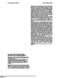
3.2.1.1.1 Population Population is one of the most important exogenous variables of the GINFORS model. We directly take the population forecast for the SSP1 scenario (comp. Figure 3.2; IIASA 2013). For all 39 countries a differentiation of three age groups is given in GINFORS: 0-14 years, 14 to 65 years, over 65 years. Total world population will reach in this forecast 8.45 billion people in 2050, which is an increase of about 23 % in four decades. As Figure 3.4 shows is this development accompanied by an aging process: The share of the over 65 rises and the share of the youngest group is falling.
28
D3-4 – Integration of top-down and bottom-up analyses
population
age group 0-14
age group 65+
age group 15 - 64
2049
2046
2043
2040
2037
2034
2031
2028
2025
2022
2019
2016
2013
2010
2007
2004
2001
1998
1995
9.000.000 8.000.000 7.000.000 6.000.000 5.000.000 4.000.000 3.000.000 2.000.000 1.000.000 0
Figure 3.4: The development of total world population (1000 persons) and age groups in the SSP1 case until 2050 (Source: IIASA 2013 & GINFORS ToPDAd)
Total EU population will increase by about 50 mill people, levelling at 554 million inhabitants in 2050. Nonetheless, the country-specific projections for the EU Member States are quite different as Error! Reference source not found. indicates. Especially for the Eastern European Countries a decrease in population has been assumed.
29
D3-4 – Integration of top-down and bottom-up analyses
Country Austria Belgium Cyprus Estonia Finland France Germany Greece Ireland Italy Luxembourg Malta Netherlands Portugal Slovak Republic Slovenia Spain Bulgaria Czech Republic Denmark Hungary Latvia Lithuania Poland Romania Sweden United Kingdom
2010 - 2020 2020 - 2030 2030 - 2040
0,39 0,55 1,17 -0,08 0,50 0,72 0,00 0,12 1,22 0,23 1,60 0,35 0,42 0,24 0,29 0,35 0,60 -0,60 0,49 0,50 -0,20 -0,59 -0,44 0,07 -0,37 0,86 0,68
0,36 0,52 0,88 -0,14 0,48 0,61 0,02 0,03 0,96 0,11 1,35 0,18 0,42 0,22 0,18 0,26 0,35 -0,52 0,36 0,55 -0,16 -0,55 -0,52 -0,06 -0,49 0,83 0,61
0,29 0,48 0,63 -0,07 0,39 0,55 -0,01 0,07 0,86 0,10 1,19 -0,04 0,33 0,22 0,01 0,25 0,38 -0,44 0,26 0,50 -0,18 -0,54 -0,64 -0,22 -0,57 0,73 0,54
2040 - 2050
0,23 0,42 0,44 -0,00 0,37 0,46 -0,04 0,03 0,75 0,03 1,00 -0,20 0,25 0,15 -0,03 0,24 0,31 -0,46 0,29 0,46 -0,20 -0,56 -0,71 -0,26 -0,72 0,74 0,50
Table 3.1: Development of population (average annual growth rate per decennium) for all EU27 Member States in the SSP1 case (global sustainability) until the year 2050. Source: IIASA 2013 & GINFORS ToPDAd
3.2.1.1.2 World market extraction prices The world market prices of coal, gas and oil as well as the real world market prices for ores, non-metallic minerals and agricultural products are also exogenous model variables. All world market prices are measured in constant US-dollars. Thus, their nominal developments are further driven by (endogenous) US-price dynamics. Fossil fuel prices have been aligned to information provided by IEA Energy Technology Perspectives (ETP) (IEA, 2012). Schaeffer and van Vuuren (2012) compared the ETP and the 30
D3-4 – Integration of top-down and bottom-up analyses RCP scenarios. They indicate that the ETP 2DS scenario corresponds closely with the RCP2.6 concentration pathway, so the ETP 2DS prices for fossil fuels have been implemented in our GINFORS simulation. Figure 3.5 shows the resulting development of the world market prices in constant dollars for coal, oil and gas. The dimensions are for oil 2010 USD/bbl, for Coal 2010 USD/tonne and for gas 2010 USD/Mbtu.
120 100 80 60 40 20
coal
oil
2050
2048
2046
2044
2042
2040
2038
2036
2034
2032
2030
2028
2026
2024
2022
2020
2018
2016
2014
2012
2010
0
gas
Figure 3.5: World market extraction prices for coal, oil and gas in constant 2010 dollars in the RCP2.6/SSP1 case (global sustainability), (Source: IEA 2012 & GINFORS ToPDAd)
The coal price is falling by 40% until 2050 against 2010. The oil price in 2050 is only 12 % higher than in 2010. The gas price will be the same until 2030 and will then slightly reduce. The logic for these developments is clear. In the 2 DS scenario the reduction of fossil fuel demand will be the greatest for the most carbon intensive fuel, which means that this fuel has the strongest price reductions. 3.2.1.2 Climate policy A "holistic" set of climate policy instruments has been carefully applied in order to trace the CO2 emission pathways of the RCP2.6 scenario. It is assumed that EU Member States install a flexible supply side management for the emissions trading system (ETS), which allows a long run rise of the carbon price. For the other sectors of EU economies, a carbon tax will be introduced with a recycling of the specific tax revenue to the paying sector. In electricity production a rising quota for the total of renewables will be introduced. We assume that the suppliers of electricity have the obligation to produce a certain percentage by renewables. This total share of renewables is rising from its target values in 2020 to 90 % in 2050. There remains a rest of fossil fuel production that may be necessary for safety reasons. The choice of 31
D3-4 – Integration of top-down and bottom-up analyses the renewable technologies is depending from the historic structures and the development of the relative unit costs of the different technologies. This modelling approach has the advantage that its results can be interpreted either as the outcome of a quota system or as a classic feed in tariff- system with the time paths of the unit costs of the different technologies and the mark-ups of the electricity sector as the guaranteed tariffs. For the level of nuclear we overtake the development of a reference scenario presented by the European Commission (2013). A radical reduction of GHG emissions, local air pollution, and traffic noise can be reached by e-mobility. One aspect of e-mobility – the development of railroad services - will be positively influenced by the carbon price. Further we assume the introduction of binding emission standards for new cars and taxation of fossil fuel burning engines, which is used for subsidies for the use of hybrid and electric cars, so that industries and households in total are not hit by this taxation. Further the use of electric cars is favoured in cities by better parking conditions, exemptions from city taxes etc. In the transport sector a complex policy program has to be implemented using economic instruments, information instruments and regulations to achieve an 80% for electricity in energy consumption of land transport. The EU roadmap and the energy concept of the German government for 2050 give the improvement of the energy efficiency of buildings an important role (Prognos, 2013). We assume that subsidies for the investment in energy efficiency of buildings reach a renovation rate of 3% per year. Given these assumptions, the EU27 meets the roadmap targets (European Commission 2011a, b, c and 2013) for CO2 emissions in the global sustainability scenario. In the non-EU countries, a carbon tax will be introduced for all sectors. Quotas for renewables in electricity production as well as measures in favor of e-mobility evolve in the same manner as in EU Member States. For a sufficient reduction of the carbon intensity of basic industries, it is necessary for all countries that an information program raises material efficiency on all stages of production, especially in small and medium sized firms. So the firma at the end of the supply chain use fewer materials, which means less steel, ceramics, chemicals etc.; products whose production processes emit much carbon. A detailed motivation and description concerning the specific design of the instruments within the climate policy mix under a global cooperation policy regime is given by Meyer, Meyer and Distelkamp (2014).
3.2.1.3 Fiscal policy and public debt Generally all tax rates on income and wealth, goods purchases and production and also the rates for the contributions to social security are constant. Government expenditure is explained by the disposable income of the government.
32
D3-4 – Integration of top-down and bottom-up analyses Since financial markets react on rising debt/GDP ratios with turbulences which have severe impacts on the development of the real economy, in our long run simulations we cannot ignore an active fiscal policy which may be necessary to control public debt. To avoid unrealistic results for the long run development of the world economy, an adjustment mechanism has been modelled, which reduces government expenditures, if a critical value of net borrowing as a percentage of GDP is reached. For EU countries this critical value is 3 %, for the non EU countries it is 5 %.3
3.2.2
Simulation results
3.2.2.1 Economic developments GINFORS derives GDP developments endogenously from supply and demand effects, which are mutually interrelated via global trade. Therefore, for all 38 countries as well as the region “rest of the world” (RoW), GDP is an endogenous variable which is based on aggregated value added developments in the 35 sectors of each national economy. To bring GINFORS GDP projections more into line with those GDP pathways available at the IIASA SSP database, the endogenously projected GDP developments thus had to be adjusted in a complex sequence of country calibrations: The original SSP calculations rest on purchasing power parity values whereas GINFORS accounts for usual monetary values. Thus, an explicit adoption of the figures reported by Chateau and Dellink (2012) appears virtually impossible. Nevertheless, their implied development prospects can of course be mirrored by an adjustment of the simulated real GDP growth rates to the implied growth rates of SSP database figures. We followed this approach in our calibration sequence.4 Accordingly, relative economic performance across countries and RoW seems closely aligned to the reported SSP-figures. However, one has to be aware that these model interventions tend to inflate our economic outcomes. Figure 3.6 shows the projected – SSP1 conform – global GDP growth pathway (with an extremely high average growth rate during the whole period from about more than 3.7 %) and the growth pathways for the EU27 (+ 2.0 %), China (+ 5.6 %) and the USA (+ 2.2 %). 3
Due to the mid-term analysis perspective of gradual climate change effects (and ignoring effects of extreme weather events) on economy till 2050 the consequences of climate change induced major repair or reconstruction costs for public finance stability have not been taken into account. The latter has more relevance for a long-term analysis. 4
The calibration process follows a ranking of the size of the economies. In this way the feedback effects of international trade could be reduced. We calibrated the GDP of the twenty most important economies including the major European countries Germany, France, UK by influencing final demand. In a next step we adjusted “rest of the world” so that the world total could be met. In a third step the smaller European countries were calibrated adjusting their trade shares.
33
D3-4 – Integration of top-down and bottom-up analyses Figure 3.7 displays how the GDP development of these three regions is related to the projected global GDP development. It becomes obvious that these three regions will realize a loss of relevance on the real World GDP from 60 % (2010) to 40 % (2050). 200.000
180.000
160.000
140.000
120.000
100.000
80.000
60.000
40.000
20.000
world
EU-27
China
2049
2046
2043
2040
2037
2034
2031
2028
2025
2022
2019
2016
2013
2010
2007
2004
2001
1998
1995
0
USA
Figure 3.6: GDP in constant 1995 dollars for the world economy, the EU27, China and the USA in the RCP2.6/SSP1 case (global sustainability) until 2050, (Source: GINFORS ToPDAd)
35%
30%
25%
20%
15%
10%
5%
EU-27
China
2049
2046
2043
2040
2037
2034
2031
2028
2025
2022
2019
2016
2013
2010
2007
2004
2001
1998
1995
0%
USA
Figure 3.7: Country-specific real GDP shares to world GDP for EU27, China and the USA in the RCP2.6/SSP1 case (global sustainability) until 2050, (Source: GINFORS ToPDAd)
Table 3.2 shows the country-specific development of GDP until 2050 for all 27 EU Member States.
34
D3-4 – Integration of top-down and bottom-up analyses
Country Austria Belgium Cyprus Estonia Finland France Germany Greece Ireland Italy Luxembourg Malta Netherlands Portugal Slovak Republic Slovenia Spain Bulgaria Czech Republic Denmark Hungary Latvia Lithuania Poland Romania Sweden United Kingdom
2010 - 2020 2020 - 2030 2030 - 2040
2,25 1,96 0,71 4,28 2,19 1,57 1,13 0,29 2,07 0,45 2,32 1,71 1,69 0,03 2,07 1,28 0,77 3,34 2,97 1,17 1,11 3,97 3,78 3,61 3,23 2,98 1,94
1,71 1,74 1,62 2,50 1,84 1,99 1,75 1,19 2,42 1,54 2,57 3,01 2,06 1,45 2,63 2,71 1,39 3,76 3,52 2,23 2,79 2,87 1,71 2,52 3,17 2,56 2,24
1,47 2,04 3,52 2,58 2,44 2,65 1,48 3,63 2,26 2,01 2,69 2,91 1,87 2,82 3,14 2,03 1,41 3,35 3,41 2,16 2,05 2,67 2,14 2,00 3,00 2,01 2,71
2040 - 2050
1,75 1,89 2,56 2,03 1,30 1,78 1,52 1,48 1,22 1,42 0,65 1,52 1,48 1,43 1,61 1,45 1,73 1,76 2,14 1,41 2,35 1,29 1,06 0,78 1,78 1,83 2,15
Table 3.2: Development of real gross domestic product (GDP) (average annual growth rate per decennium) for all EU27 Member States in the RCP2.6/SSP1 case (global sustainability) until the year 2050. Source: GINFORS ToPDAd
35
D3-4 – Integration of top-down and bottom-up analyses
Annex 1 displays the development of all demand-side components of GDP (private consumption, government consumption, exports and imports) as well as disposable income of private households in full detail for all 27 EU Member States. 3.2.2.2 Electricity production Because of the climate policy assumptions and the assumed high global GDP growt, the electricity production will globally expand with an average annual growth rate of 3.6 %, for the EU27 Figure 3.8 further shows a development with an average annual growth rate of 2.1 %. The average annual growth rate of electricity production for the world as well as for the EU27 equals the related GDP growth rate. 350.000.000
300.000.000
250.000.000
200.000.000
150.000.000
100.000.000
50.000.000
world
2049
2046
2043
2040
2037
2034
2031
2028
2025
2022
2019
2016
2013
2010
2007
2004
2001
1998
1995
0
EU-27
Figure 3.8: The development of electricity production in TJ in the world and the EU27 in the RCP2.6/SSP1 case (global sustainability) until 2050, (Source: GINFORS ToPDAd)
The following two figures show how the energy carrier mix in electricity production will change at the global level and at EU27 level because of a global sustainability oriented climate policy. It gets obvious that a global sustainable climate policy in direction to a global low-carbon economy with globally reduced CO2 emission will affect tremendously the electricity production. In such a world renewables will have a dominating role which substitute the “classical” energy carriers.
36
D3-4 – Integration of top-down and bottom-up analyses 100,0% 90,0% 80,0% 70,0%
Renewables
60,0%
Nuclear
50,0%
Coal
40,0%
Gas
30,0%
Oil
20,0% 10,0%
2049
2046
2043
2040
2037
2034
2031
2028
2025
2022
2019
2016
2013
2010
0,0%
Figure 3.9: The development of the shares of energy carriers in electricity production in TJ in the world in the RCP2.6/SSP1 case (global sustainability), (Source: GINFORS ToPDAd)
90,0% 80,0% 70,0% 60,0%
Renewables
50,0%
Nuclear
40,0%
Coal
30,0%
Gas
20,0%
Oil
10,0%
2049
2046
2043
2040
2037
2034
2031
2028
2025
2022
2019
2016
2013
2010
0,0%
Figure 3.10: The development of the shares of energy carriers in electricity production in TJ for EU27 in the RCP2.6/SSP1 case (global sustainability), (Source: GINFORS ToPDAd)
3.2.2.3 CO2 emissions In Figure 3.1 it was shown that within the CO2 emission pathway of RCP2.6 it has been assumed that the emissions will reach its maximum already in 2020 and then fall strongly till 2050 reaching a level, which is about 66 % lower than the actual one. In 2050 the global target of 12.4 Gt CO2 should be reached.
37
D3-4 – Integration of top-down and bottom-up analyses As already mentioned, a very strong global climate policy for reaching extremely reduced CO2 emissions has been assumed in the GINFORS modelling exercise for reaching extremely reduced global CO2 emissions. Due to the extremely high GDP growth rates as projected for emerging and developing countries within the IISAS SSP1 database we were not able to find a GINFORS projection outcome – despite of a huge number of model simulation runs with alternative stronger climate policy set-ups – which reach the global CO2 target of 12.4 Gt. Figure 3.11 presents the CO2 emission pathways for the world, the EU27, China and the USA as projected within the fully integrated dynamic global economic-energy-environment (3E) model GINFORS under the assumptions of a globally accepted strong CO2 emission reducing climate policy at national country level and meeting the GDP pathways as projected within the IIASA SSP1 database.
40.000.000 35.000.000 30.000.000 25.000.000 20.000.000 15.000.000 10.000.000 5.000.000
EU-27
China
USA
2049
2046
2043
2040
2037
2034
2031
2028
2025
2022
2019
2016
2013
2010
2007
2004
2001
1998
1995
0
World
Figure 3.11: The development of the CO2 emissions in kilo tons for the EU, China and the USA in the RCP2.6/SSP1 case (global sustainability), (Source: GINFORS ToPDAd)
Despite the high GDP growth (average annual growth + 3.7 %) during the projection period 2013 – 2050 the CO2 emissions will decrease (average annual growth – 0.8 %). In total the CO2 emissions will be reduced for nearly 5.5 Gt to 23.6 Gt. Although this is far away from the targeted goal of 12.4 Gt, it is a quite strong reduction of CO2 emission against the backdrop of a economically strong growing world economy. The latter gets clearer when looking at the development of country-specific CO2 emissions in relation to the global CO2 emissions.
38
D3-4 – Integration of top-down and bottom-up analyses 35,0% 30,0%
25,0% 20,0%
15,0% 10,0% 5,0%
EU-27
China
2049
2046
2043
2040
2037
2034
2031
2028
2025
2022
2019
2016
2013
2010
2007
2004
2001
1998
1995
0,0%
USA
Figure 3.12: Shares of country-specific CO2 emissions to the global CO2 emissions for EU27, China and the USA in the RCP2.6/SSP1 case (global sustainability) until 2050, (Source: GINFORS ToPDAd)
Finally the following table shows the country-specific development of CO2 emissions until 2050 for all 27 EU Member States.
39
D3-4 – Integration of top-down and bottom-up analyses
Country Austria Belgium Cyprus Estonia Finland France Germany Greece Ireland Italy Luxembourg Malta Netherlands Portugal Slovak Republic Slovenia Spain Bulgaria Czech Republic Denmark Hungary Latvia Lithuania Poland Romania Sweden United Kingdom
2010 - 2020 2020 - 2030 2030 - 2040
-0,70 1,71 -0,91 1,14 -0,70 -0,90 -1,22 -1,04 -1,94 -2,30 -0,99 -2,36 -2,11 -0,29 -1,19 3,21 -0,76 1,02 -0,92 -1,45 -1,49 -0,23 0,33 0,27 3,56 -1,06 -1,93
-0,41 3,74 0,61 -1,55 -2,90 -1,47 -1,26 -1,49 -1,66 -1,27 -0,38 -1,29 -0,73 -0,59 -1,27 1,31 -0,98 -1,00 -3,58 -0,65 -2,63 -1,19 -4,71 -2,79 -1,02 -1,63 -0,96
-0,71 0,13 1,02 -2,80 -2,46 -1,94 -2,15 -1,26 -2,22 -1,84 -0,91 -2,66 -1,20 -0,77 0,09 -2,13 -2,20 -8,13 -5,17 -1,57 -0,73 -1,75 -3,54 -3,94 -2,35 -1,84 -2,11
2040 - 2050
-1,29 -2,75 -2,09 -7,71 -2,68 -2,48 -4,00 -5,76 -4,89 -3,76 -4,06 -9,03 -3,34 -4,14 -0,61 0,32 -4,60 -2,83 -2,29 -4,03 -3,96 -4,75 -2,54 -4,11 -6,12 -2,30 -3,91
Table 3.3: Development of total carbon dioxide (CO2) emissions (average annual growth rate per decennium) for all EU27 Member States in the RCP2.6/SSP1 case (global sustainability) until the year 2050. Source: GINFORS ToPDAd
3.2.2.4 Employment GINFORS calculates labour demand in the dimension of hours worked based on sectoral production and the real wage rate – both being endogenous – for 38 countries in 35 industries. The step from hours worked to the number of persons employed is done by division with the hours worked per person in that industry and country. To be cautious with our estimation of employed persons we take the actual numbers of the hours worked per person as constant. 40
D3-4 – Integration of top-down and bottom-up analyses Figure 3.13 shows the aggregate employment quota (quota between the number of persons employed and the total population) for EU27. Actually, 45 % of the total population is employed. Until 2050 this number will continuously rise to 59.7 %. Labour will be a much scarcer factor of production than today. The reason will be the demographic change, which reduces the number of persons in the age group 15-65. This feeds back into the wage determination pushing the wage rate. The model finds a solution of these interdependencies with a reduction of employment due to the rise of labour productivity, which is weaker than the reduction on the supply side of the labour market.
70% 60% 50% 40% 30% 20% 10% 2049
2046
2043
2040
2037
2034
2031
2028
2025
2022
2019
2016
2013
2010
2007
2004
2001
1998
1995
0%
employment quota
Figure 3.13: The development of the employment quota in EU27 in the RCP2.6/SSP1 case (global sustainability) until 2050, (Source: GINFORS ToPDAd)
Figure 3.13 shows that the employment quota in EU27 rises continuously and compared with the actual situation. This has to be interpreted as a tension at the labour market. The interpretation is underlined by the fact, that the hours worked per person have been held constant. If actual trends of the reduction of hours worked per person would have been assumed, the graph would have been even much steeper. Caution is needed in interpreting these results, because these effects are very different in the member states. Finally the following table shows the country-specific development of employment until 2050 for all 27 EU Member States.
41
D3-4 – Integration of top-down and bottom-up analyses
Country Austria Belgium Cyprus Estonia Finland France Germany Greece Ireland Italy Luxembourg Malta Netherlands Portugal Slovak Republic Slovenia Spain Bulgaria Czech Republic Denmark Hungary Latvia Lithuania Poland Romania Sweden United Kingdom
2010 - 2020 2020 - 2030 2030 - 2040
1,36 1,56 -0,36 2,69 1,05 0,71 0,14 -0,86 -0,60 -0,59 1,51 -1,69 0,56 -0,59 -0,57 0,27 0,06 -0,27 0,24 0,54 0,67 1,56 1,79 0,67 3,79 1,57 0,74
0,94 1,80 0,39 1,08 0,15 1,13 0,77 -0,70 -0,14 1,05 1,56 0,35 0,88 0,03 0,59 1,95 0,51 0,24 0,79 1,29 2,28 1,22 -0,02 -0,16 0,83 1,60 1,64
0,95 2,27 2,85 1,64 1,17 1,62 1,10 2,14 1,15 1,91 2,40 1,10 1,27 1,48 1,85 1,56 0,70 0,14 0,90 1,25 1,33 1,50 1,00 -0,25 0,89 1,52 2,10
2040 - 2050
1,19 1,09 1,87 0,70 0,64 0,93 1,21 1,16 0,48 1,07 1,52 -0,09 0,99 0,41 0,93 0,61 0,99 -0,53 0,25 0,58 1,18 0,20 0,10 -1,33 0,02 1,61 1,43
Table 3.4: Development of employment (average annual growth rate per decennium) for all EU27 Member States in the RCP2.6/SSP1 case (global sustainability) until 2050. Source: GINFORS ToPDAd
3.3
RCP4.5/SSP4 (Divided World)
The scenario “Divided World” assumes that the international community fails to establish a climate treaty, but that there is at least some uncoordinated action: The European countries retain the strong reduction targets for climate gases (80% against the emissions of 1990) consistent with the 2 degrees warming target. The Non-European countries install some climate policy instruments with a reduced intensity resulting in a GHG concentration path which is consistent with the RCP 4.5 development described by Clarke et al., 2007. We could interpret this constellation till 2050 as a delayed reaction of the Non-European countries, 42
D3-4 – Integration of top-down and bottom-up analyses which may after 2050, follow the EU example. This perspective might give a motivation for EU countries to go in front although in 2050 the 2 degrees Celsius emission pathway will probably not be met. Depending from the development after 2050 global warming in 2100 will be somewhere between 2 and 2.6 degrees. 3.3.1
Scenario setup
3.3.1.1 Exogenous assumptions
3.3.1.1.1 Population As already mentioned, is population one of the most important exogenous variables of the model GINFORS. We directly take the population forecast for the SSP4 scenario (comp. Figure 3.2; IIASA 2013), shown in Figure 3.14.
population
age group 0-14
age group 65+
age group 15 - 64
2049
2046
2043
2040
2037
2034
2031
2028
2025
2022
2019
2016
2013
2010
2007
2004
2001
1998
1995
10.000.000 9.000.000 8.000.000 7.000.000 6.000.000 5.000.000 4.000.000 3.000.000 2.000.000 1.000.000 0
Figure 3.14: The development of total world population (1000 persons) and age groups in the SSP4 case until 2050, (Source: IIASA 2013 & GINFORS ToPDAd)
In this scenario, total world population will reach 9.12 billion people in 2050, which is an increase of about 33 % in four decades. This – in comparison to SSP1, about 0.6 billion higher number in 2050 – development is accompanied by an aging process: The share of the over 65 rises whereas the share of the youngest group is more or less stable. EU population will only increase slightly from 502 mill. (2010) to 509 mill. inhabitants in 2050. In comparison to SSP1, this is 0.46 million lower in 2050. This has also implications for the country-specific projections for the EU Member States, which are also quite different as Error! Reference source not found. indicates. 43
D3-4 – Integration of top-down and bottom-up analyses
Country Austria Belgium Cyprus Estonia Finland France Germany Greece Ireland Italy Luxembourg Malta Netherlands Portugal Slovak Republic Slovenia Spain Bulgaria Czech Republic Denmark Hungary Latvia Lithuania Poland Romania Sweden United Kingdom
2010 - 2020 2020 - 2030 2030 - 2040
0,29 0,42 1,15 -0,18 0,37 0,62 -0,10 0,02 1,11 0,14 1,50 0,33 0,32 0,15 0,20 0,25 0,52 -0,63 0,38 0,37 -0,30 -0,63 -0,48 -0,01 -0,37 0,73 0,57
0,16 0,27 0,85 -0,33 0,21 0,41 -0,19 -0,15 0,74 -0,07 1,17 0,09 0,20 0,05 -0,01 0,07 0,20 -0,58 0,16 0,27 -0,37 -0,63 -0,60 -0,24 -0,53 0,56 0,39
0,03 0,16 0,57 -0,35 0,04 0,30 -0,28 -0,17 0,57 -0,13 0,96 -0,14 0,05 -0,01 -0,24 -0,01 0,17 -0,55 0,00 0,15 -0,46 -0,66 -0,76 -0,48 -0,66 0,40 0,25
2040 - 2050
-0,09 0,02 0,39 -0,35 -0,05 0,15 -0,38 -0,28 0,40 -0,26 0,73 -0,30 -0,10 -0,13 -0,35 -0,08 0,04 -0,56 -0,02 0,05 -0,53 -0,72 -0,86 -0,59 -0,85 0,35 0,15
Table 3.5: Development of population (average annual growth rate per decennium) for all EU27 Member States in the SSP4 case (divided world) until the year 2050. Source: IIASA 2013 & GINFORS ToPDAd
44
D3-4 – Integration of top-down and bottom-up analyses
3.3.1.1.2 World market extraction prices Fossil fuel prices have been aligned to information provided by IEA Energy Technology Perspectives (ETP) (IEA, 2012). Schaeffer and van Vuuren (2012) indicate that the ETP 2DS scenario corresponds closely with the RCP4.5 concentration pathway, so the ETP 4DS prices for fossil fuels have been implemented in this GINFORS simulation. Figure 3.15 shows the resulting development of the world market prices in constant dollars for coal, oil and gas.
140 120 100 80 60 40 20
coal
oil
2050
2048
2046
2044
2042
2040
2038
2036
2034
2032
2030
2028
2026
2024
2022
2020
2018
2016
2014
2012
2010
0
gas
Figure 3.15: World market extraction prices for coal, oil and gas in constant 2010 US$ per specific quantity unit in the RCP4.5/SSP4 case (divided world) until 2050, (Source: IEA 2012 & GINFORS ToPDAd)
The coal price is rising by 10 % until 2050 against 2010. The oil price in 2050 is about 50 % higher than in 2010. The real gas price rises until the mid of the 2030-ies by 150% and then tend to be more or less stable until 2050.
3.3.1.2 Climate policy A "holistic" set of climate policy instruments has been has been carefully applied in order to trace the CO2 emission pathways of the RCP4.5 scenario. The EU27 countries will implement the same policy mix as in the “global sustainability” scenario (compare Section 3.2.1.2) to reach an 80 % reduction of CO2 in relation to the 1990 numbers. The other countries in the world may not introduce the cap and trade system. This seems to be plausible, because this instrument demands some administrative costs and the feasibility of the instrument could be problematic. On the other side the introduction of e-mobility could be 45
D3-4 – Integration of top-down and bottom-up analyses interesting for the non-European countries, because the markets for cars are very strongly internationally linked so that the others might follow the European fore runners. Subsidies for the investment in buildings are not part of the climate policy of the non-European countries. Quotas for renewables in electricity production are a central part of their climate policy, but the target is only to reach a share of 70 %. The information policy for rising material efficiency will be accepted by the other countries, because the direct effect of the consulted firms is a cost reduction.
3.3.1.3 Fiscal policy and public debt Fiscal policy and public debt follows the procedure explained in Section 2.3.1.3. It is assumed that a sustainable fiscal and budgetary policy is implemented at the national country level.
3.3.2
Simulation results
3.3.2.1 Economic developments As already mentioned, GINFORS derives GDP developments endogenously in a bottom-up procedure from supply and demand effects, which are mutually interrelated via global trade. Figure 3.16 shows the projected – SSP4 conform – global GDP growth pathway (with a high average growth rate during the whole period from about more than 2.9 %) and the growth pathways for the EU27 (+ 1.8 %), China (+ 4.0 %) and the USA (+ 1.9 %). In comparison to SSP1, the world [EU27] GDP is about 38 400 [2 600] billion US$ lower in 2050. Despite a higher population growth, the projected GDP growth in this SSP scenario is lower compared with the global sustainability scenario (compare section 3.2.2.1).5
5
To bring GINFORS GDP projections in line with the GDP pathways published within the IIASA SSP database by different socioeconomic models with a CGE foundation, the endogenously by GINFORS projected GDP developments have been adjusted in a complex sequence of country calibrations, which is described in section Error! Reference source not found.
46
D3-4 – Integration of top-down and bottom-up analyses 160.000
140.000
120.000
100.000
80.000
60.000
40.000
20.000
world
EU-27
China
2049
2046
2043
2040
2037
2034
2031
2028
2025
2022
2019
2016
2013
2010
2007
2004
2001
1998
1995
0
USA
Figure 3.16: GDP in constant 1995 dollars for the world economy, the EU27, China and the USA in the RCP4.5/SSP4 case (divided world) until 2050, (Source: GINFORS ToPDAd)
Finally, Table 3.6 shows the country-specific development of GDP until 2050 for all 27 EU Member States.
47
D3-4 – Integration of top-down and bottom-up analyses
Country Austria Belgium Cyprus Estonia Finland France Germany Greece Ireland Italy Luxembourg Malta Netherlands Portugal Slovak Republic Slovenia Spain Bulgaria Czech Republic Denmark Hungary Latvia Lithuania Poland Romania Sweden United Kingdom
2010 - 2020 2020 - 2030 2030 - 2040
1,81 1,80 0,64 4,23 1,77 1,61 1,64 -2,07 1,94 0,12 2,23 2,46 1,53 -0,77 2,60 1,26 0,72 2,70 2,95 1,25 0,84 3,74 2,98 3,31 2,62 2,71 2,07
1,77 1,41 3,72 2,42 1,96 1,72 1,15 3,01 2,39 1,76 1,94 1,37 1,32 1,70 2,78 2,28 0,86 2,73 3,25 1,70 2,66 2,27 1,60 2,31 2,81 1,88 1,75
1,52 1,69 1,05 2,38 1,76 2,41 1,12 2,26 1,93 1,44 1,72 2,54 1,50 1,89 2,33 1,82 1,19 1,60 2,71 1,70 2,06 1,67 0,86 1,97 1,63 2,28 1,99
2040 - 2050
1,21 1,74 1,68 1,24 0,86 1,45 1,04 1,80 0,96 1,15 1,08 1,82 1,27 1,36 1,25 0,80 1,31 1,44 1,66 1,79 0,87 0,88 0,58 0,71 0,82 1,52 1,52
Table 3.6: Development of real gross domestic product (GDP) (average annual growth rate per decennium) for all EU27 Member States in the RCP4.5/SSP4 case (divided world) until the year 2050. Source: GINFORS ToPDAd
Annex 1 displays the development of all demand-side components of GDP (private consumption, government consumption, exports and imports) as well as disposable income of private households in full detail for all 27 EU Member States. 3.3.2.2 Electricity production Electricity production will globally expand with an average annual growth rate of 3.1 %, for the EU27 the Figure 3.17 further shows a development with an average annual growth rate of 1.9 %. The average annual growth rate of electricity production for the World is a little bit 48
D3-4 – Integration of top-down and bottom-up analyses higher than the related GDP growth rate (2.9 %). The same is also the case for the related EU27 GDP growth rate (1.8 %).
300.000.000
250.000.000
200.000.000
150.000.000
100.000.000
50.000.000
world
2049
2046
2043
2040
2037
2034
2031
2028
2025
2022
2019
2016
2013
2010
2007
2004
2001
1998
1995
0
EU-27
Figure 3.17: The development of electricity production in TJ in the world and the EU27 in the RCP4.5/SSP4 case (divided world) until 2050, (Source: GINFORS ToPDAd)
Figures 3.18 and 3.19 show how the energy carrier mix in electricity production will change at the global level and at EU27 level on account of a sustainability oriented climate policy in a divided world. It gets obvious that such a bisected climate policy with different a different low-carbon economy policy mix at EU27 and non EU-level affects also the related electricity production.
49
D3-4 – Integration of top-down and bottom-up analyses 80,0% 70,0% 60,0% Renewables
50,0%
Nuclear
40,0%
Coal
30,0%
Gas
20,0%
Oil
10,0%
2049
2046
2043
2040
2037
2034
2031
2028
2025
2022
2019
2016
2013
2010
0,0%
Figure 3.18: The development of the shares of energy carriers in electricity production in TJ in the world in the RCP4.5/SSP4 case (divided world) until 2050, (Source: GINFORS ToPDAd)
90,0% 80,0% 70,0% 60,0%
Renewables
50,0%
Nuclear
40,0%
Coal
30,0%
Gas
20,0%
Oil
10,0%
2049
2046
2043
2040
2037
2034
2031
2028
2025
2022
2019
2016
2013
2010
0,0%
Figure 3.19: The development of the shares of energy carriers in electricity production in TJ for EU27 in the RCP4.5/SSP4 case (divided world) until 2050, (Source: GINFORS ToPDAd)
3.3.2.3 CO2 emissions Figure 3.1 showed that within the CO2 emission pathway of RCP4.5 it is assumed that the emissions will constantly grow for the next three decades and reaches its maximum in 2043 with 42.1 Gt. In 2050 the global target of 41.4 Gt CO2 should be reached. Figure 3.20 presents the CO2 emission pathways for the world, the EU27, China and the USA as projected within the fully integrated dynamic global economic-energy-environment (3E) 50
D3-4 – Integration of top-down and bottom-up analyses model GINFORS under the RCP4./SSP4 (divided world) case assumptions. The global CO2 emission pathway as assumed for RCP4.5 is met by the suggested climate policy mix under the SSP4 conditions.
45.000.000 40.000.000 35.000.000 30.000.000 25.000.000 20.000.000 15.000.000 10.000.000 5.000.000
EU-27
China
USA
2049
2046
2043
2040
2037
2034
2031
2028
2025
2022
2019
2016
2013
2010
2007
2004
2001
1998
1995
0
World
Figure 3.20: The development of the CO2 emissions in kilo tons for the EU, China and the USA in the RCP4.5/SSP4 case until 2050 (divided world), (Source: GINFORS ToPDAd)
Finally, Table 2.7 shows the country-specific development of CO2 emissions until 2050 for all 27 EU Member States.
51
D3-4 – Integration of top-down and bottom-up analyses
Country Austria Belgium Cyprus Estonia Finland France Germany Greece Ireland Italy Luxembourg Malta Netherlands Portugal Slovak Republic Slovenia Spain Bulgaria Czech Republic Denmark Hungary Latvia Lithuania Poland Romania Sweden United Kingdom
2010 - 2020 2020 - 2030 2030 - 2040
-1,13 1,59 -1,21 1,27 -0,93 -0,99 -0,87 -2,15 -2,10 -2,73 -1,06 -1,78 -2,37 -0,63 -0,54 3,14 -0,96 0,33 -0,98 -1,59 -1,62 -0,44 -0,11 0,06 2,87 -1,10 -1,84
-0,53 3,43 1,38 -1,39 -2,71 -1,75 -1,38 -0,52 -1,48 -1,28 -0,75 -2,40 -1,30 -0,72 -0,80 0,82 -1,45 -2,06 -3,91 -1,06 -2,63 -1,61 -4,71 -2,86 -1,47 -1,75 -1,09
-0,70 -0,74 -0,97 -3,06 -2,96 -2,09 -2,42 -2,16 -2,54 -2,21 -1,54 -3,80 -1,86 -1,71 -0,97 -3,36 -2,67 -9,71 -5,48 -2,31 -0,89 -2,62 -3,70 -4,20 -3,72 -1,23 -2,52
2040 - 2050
-1,99 -2,92 -2,65 -8,00 -2,61 -2,87 -4,12 -5,63 -4,95 -3,79 -2,96 -8,67 -3,51 -4,16 -1,24 0,38 -4,72 -3,08 -2,51 -4,17 -4,91 -4,89 -2,39 -4,59 -6,68 -2,37 -4,51
Table 3.7: Development of total carbon dioxide (CO2) emissions (average annual growth rate per decennium) for all EU27 Member States in the RCP4.5/SSP4 case (divided world) until 2050. Source: GINFORS ToPDAd
3.3.2.4 Employment Figure 3.13 shows the aggregate employment quota (quota between the number of persons employed and the total population) for EU27. Actually, 45 % of the total population are employed, until 2050 this number will continuously rise up to 60.4 %. Labour will be a much scarcer factor of production than today.
52
D3-4 – Integration of top-down and bottom-up analyses 70% 60% 50% 40% 30% 20% 10% 2049
2046
2043
2040
2037
2034
2031
2028
2025
2022
2019
2016
2013
2010
2007
2004
2001
1998
1995
0%
employment quota
Figure 3.21: The development of the employment quota in EU27 in the RCP4.5/SSP4 case (divided world) until 2050, (Source: GINFORS ToPDAd)
Finally, Table 3,8 shows the country-specific development of employment until 2050 for all 27 EU Member States.
53
D3-4 – Integration of top-down and bottom-up analyses
Country Austria Belgium Cyprus Estonia Finland France Germany Greece Ireland Italy Luxembourg Malta Netherlands Portugal Slovak Republic Slovenia Spain Bulgaria Czech Republic Denmark Hungary Latvia Lithuania Poland Romania Sweden United Kingdom
2010 - 2020 2020 - 2030 2030 - 2040
0,93 1,47 -0,39 2,82 0,59 0,76 0,87 -2,63 -0,82 -0,85 1,36 -1,00 0,45 -1,15 0,19 0,36 0,07 -0,66 0,23 0,68 0,47 1,40 1,12 0,46 2,37 1,57 0,82
1,10 1,50 2,59 1,25 0,52 0,97 0,86 1,52 0,63 1,51 0,88 -1,72 0,27 0,44 1,09 1,65 0,13 -0,34 0,69 0,96 2,46 0,79 -0,02 -0,15 0,39 1,24 1,18
1,08 1,52 0,57 1,34 0,64 1,44 1,04 1,35 1,22 1,33 2,47 0,11 0,93 0,63 1,24 1,16 0,55 -0,71 0,68 0,92 1,33 0,70 -0,38 0,12 -0,45 2,05 1,58
2040 - 2050
0,71 0,91 1,03 -0,12 0,20 0,62 0,83 1,32 0,50 0,75 3,31 0,23 0,90 0,20 0,38 -0,05 0,54 -0,84 0,14 0,88 -0,11 -0,11 -0,61 -1,08 -0,86 1,52 0,95
Table 3.8: Development of employment (average annual growth rate per decennium) for all EU27 Member States in the RCP4.5/SSP4 case (divided world) until the year 2050. Source: GINFORS ToPDAd
3.4
Conclusions concerning the SSP implementation approach
The global energy-environment-economy (3E) model GINFORS addressed the medium longterm view of a decarbonizing policy pathway that covered the present up till 2050. The comprehensive modelling approach maps global interrelationships between consumers, producers and investors. It accounts for imperfect markets and limited rationality of agents
54
D3-4 – Integration of top-down and bottom-up analyses and indicates the complex international feedbacks from structural changes in individual countries or changes in international trade patterns. The GDP projections within the IIASA SSP database, which have been taken as reference within the ToPDAd macroeconomic modelling, have been calculated with aggregated macroeconomic models using assumptions about future developments of factor productivity. The implicit assumption is that supply dominates demand, which is consistent in a neoclassical framework. It further excludes any impact from structural changes on the macroeconomic development. Both implications are not given in a Neo-Keynesian macroeconomic approach on which GINFORS is based. Here market imperfections and the absence of Say’s law are introduced. Therefore the adaptation of the SSP GDP developments by GINFORS has its limits, because GINFORS calculates endogenously GDP based on the interaction of supply and demand and structural change of the economy. But the useful experience was that from this perspective some of the SSP developments seemed to be rather extreme. This concerns for example the very high GDP growth in SSP1, which is combined with RCP2.6. Even our assumption of a very ambitious climate policy implemented worldwide generates for 2050 CO2 emissions of about 23 Gt, which is much more than the targeted 13 Gt within RCP2.6. From this perspective we can formulate two implications because of our global modelling exercise: On the one hand if the projected high global GDP growth within SSP1 – as it was projected jointly from the scientific working group on scenarios of the integrated assessment modeling consortium (IAMC) – should actually adjust, the RCP2.6 emission pathway will not be achieved in 2050 by far. In such a situation there will be long-term challenges of climate adaptation. On the other hand it also indicates that the theoretical concept of free combinability of all RCPs and SSPs has to be critically reflected. From our experience GDP projections should be developed in a fully integrated global 3E modelling approach on the basis of population projections, SSP storylines and RCP targets on CO2 emissions with the related climate policy mix formulated within the SPAs. By doing so GDP and CO2 emission pathways as well as the related structural change within the economic and energy system fit consistently together.6 Meyer, Meyer & Distelkamp presented in 2014 within the European Commission project CECILIA2050 the GINFORS outcome concerning macro-economic routes to 2050. The latter was endogenously projected within the GINFORS model, and – in contrast to the ToPDAd project – not finally calibrated to the GDP pathway projections published within the IIASA database.
6
Because this has not been the case for this modelling exercise within the ToPDAd project with predetermined specifications for GDP pathways also results concerning possible effects on the structure of economy are not presented.
55
D3-4 – Integration of top-down and bottom-up analyses
3.5
3.5.1
Case theme 5: Power sector adaptability in Northern Europe – macroeconomic and environmental impacts of a reduced heat demand Preliminaries
The energy system of the EU is increasingly strained by growth in demand that is running ahead of investment in new energy generation capacity. That strain will change as climate mitigation policies call for greater reliance on low-carbon, renewable energy sources, and as climate changes potentially reduce demand in winter but increasing demand in summer. ToPDAd has brought together economic, energy, climate and decision-making models to provide a glimpse into how the energy system might evolve over the coming decades and into the points of greatest vulnerability of the energy system to climate impacts. The ToPDAd project has addressed climate change and adaptation challenges for the sectors tourism, transportation and energy. The sectoral assessments has been studied in detail for seven case themes on climate adaption (ToPDAd deliverable 2.4). The assessment of macroeconomic effects of climate change impacts which have been studied in detail at sectoral level are studied now in more detail for case theme 5 on energy supply. The geographical area that is covered in the case theme 5 is presented in Figure 3.22. The case theme 5 is more thoroughly described in ToPDAd deliverables D2.3 and D2.4.
Figure 3.22: Geographical distribution of the Balmorel model (ToPDAd deliverable D2.4, 2015)
56
D3-4 – Integration of top-down and bottom-up analyses
3.5.2
Integration of sector modelling results
The sector modelling results of case theme 5 concerning the impact of climate change in RCP2.6 and RCP4.5 scenarios on the demand side for heat demand are shown in Error! Reference source not found. and Error! Reference source not found.. The estimations with the Balmorel model show that climate change leads to and overall country-specific reduction of heat demand in EU Member States of the Baltic region until 2050. The country-specific information has been consistently integrated within the GINFORS model. A reduction of heat demand in GINFORS directly affects the gross energy use for heating in private households as well as for heating within the industries of economy except the energy use for raw material based industrial process heating in the relevant industries. BASE Country Estonia Finland Germany Denmark Latvia Lithuania Poland Sweden
Year 2050 2050 2050 2050 2050 2050 2050 2050
BASE Value 7.638.000 77.145.010 180.000.000 41.341.000 9.000.000 11.000.000 120.000.000 61.171.000
RCP2.6 Value 7.217.180 75.206.170 165.487.000 38.300.550 8.537.773 10.275.628 110.908.785 57.846.100
Difference in % -5,5 -2,5 -8,1 -7,4 -5,1 -6,6 -7,6 -5,4
Table 3.9: Heat demand in 2050 for the Baltic region EU Member States estimated with the Balmorel model for the base line scenario with no climate-induced change and within the RCP2.6 low climate change scenario. Source: Perrels et al. 2015 & VTT
BASE Country Estonia Finland Germany Denmark Latvia Lithuania Poland Sweden
Year 2050 2050 2050 2050 2050 2050 2050 2050
BASE Value 7.638.000 77.145.010 180.000.000 41.341.000 9.000.000 11.000.000 120.000.000 61.171.000
RCP4.5 Value 7.110.100 74.685.500 161.995.000 37.415.730 8.422.757 10.080.946 108.227.812 56.790.500
Difference in % -6,9 -3,2 -10,0 -9,5 -6,4 -8,4 -9,8 -7,2
Table 3.10: Heat demand in 2050 for the Baltic region EU Member States estimated with the Balmorel model for the base line scenario with no climate-induced change and within the RCP4.5 moderate climate change scenario. Source: Perrels et al. 2015 & VTT
57
D3-4 – Integration of top-down and bottom-up analyses
Within GINFORS the energy, environmental and economic impacts – including all direct and indirect demand effects, price effects and income cycle effects – are analysed in full detail at the national country-level for the RCP2.6/SSP1 case (global sustainability) and the RCP4.5/SSP4 case (divided world). The result figures of this policy simulation focus on changes in GDP and CO2 emission. 3.5.2.1 Impacts for the RCP2.6/SSP1 case (global sustainability)
Country Estonia Finland Germany Denmark Latvia Lithuania Poland Sweden
2010 - 2020 2020 - 2030 2030 - 2040
0,001 0,002 0,003 0,004 0,000 0,006 0,003 0,000
-0,001 0,002 0,002 0,004 0,003 0,010 0,002 0,001
0,001 0,001 -0,000 0,001 0,001 -0,008 0,001 0,001
2040 - 2050
-0,005 -0,003 -0,004 -0,002 -0,001 0,007 -0,004 -0,002
Table 3.11: Difference of real gross domestic product (GDP) (shown as differences in average annual growth rate per decennium compared to its base line projection) due to global warming infected reduced heat demand for the Baltic region EU Member States in the RCP2.6/SSP1 case (global sustainability) until the year 2050. Source: GINFORS ToPDAd
Country Estonia Finland Germany Denmark Latvia Lithuania Poland Sweden
2010 - 2020 2020 - 2030 2030 - 2040
-0,036 -0,015 -0,039 -0,075 -0,026 -0,037 -0,042 -0,021
-0,039 -0,024 -0,045 -0,110 -0,028 -0,052 -0,065 -0,030
-0,028 -0,018 -0,039 -0,108 -0,025 -0,004 -0,078 -0,014
2040 - 2050
-0,035 0,000 -0,051 -0,089 -0,031 -0,020 -0,055 -0,014
Table 3.12: Difference of total carbon dioxide (CO2) emissions (shown as differences in average annual growth rate per decennium compared to its base line projection) due to global warming infected reduced heat demand for the Baltic region EU Member States in the RCP2.6/SSP1 case (global sustainability) until the year 2050. Source: GINFORS ToPDAd
58
D3-4 – Integration of top-down and bottom-up analyses 3.5.2.2 Impacts for the RCP4.5/SSP4 case (divided world) Country Estonia Finland Germany Denmark Latvia Lithuania Poland Sweden
2010 - 2020 2020 - 2030 2030 - 2040
0,001 0,001 0,004 0,005 0,001 0,007 0,003 0,001
-0,001 0,002 0,002 0,003 0,004 0,002 0,004 0,001
0,005 0,001 0,000 -0,000 0,005 0,050 0,003 -0,010
2040 - 2050
-0,004 -0,001 -0,002 -0,003 -0,002 -0,036 -0,008 -0,002
Table 3.13: Difference of real gross domestic product (GDP) (shown as differences in average annual growth rate per decennium compared to its base line projection) due to global warming infected reduced heat demand for the Baltic region EU Member States in the RCP4.5/SSP4 case (divided world) until the year 2050. Source: GINFORS ToPDAd
Country Estonia Finland Germany Denmark Latvia Lithuania Poland Sweden
2010 - 2020 2020 - 2030 2030 - 2040
-0,041 -0,015 -0,046 -0,091 -0,032 -0,043 -0,054 -0,029
-0,045 -0,022 -0,054 -0,138 -0,033 -0,074 -0,083 -0,041
-0,028 -0,019 -0,051 -0,125 -0,023 0,025 -0,090 -0,033
2040 - 2050
-0,037 0,004 -0,070 -0,090 -0,036 -0,039 -0,072 -0,021
Table 3.14: Difference of total carbon dioxide (CO2) emissions (shown as differences in average annual growth rate per decennium compared to its base line projection) due to global warming infected reduced heat demand for the Baltic region EU Member States in the RCP4.5/SSP4 case (divided world) until the year 2050. Source: GINFORS ToPDAd
3.5.3
Conclusions
The integration of sector results for the energy case shows that the lower climate change related country-specific heat demand within the Baltic regions has positive overall impacts on GDP due to direct demand and price effects of the reduced expenditures for heating within households and industries. This generates positive income cycle effects. In the last decade of the simulation the GDP effect gets negative. This is because the macroeconomic reaction 59
D3-4 – Integration of top-down and bottom-up analyses behaviour within a low-carbon intensive economy that is achieved at the end of the simulation period changes due to the challenging climate policy mix. The lower climate change related country-specific heat demand has positive effects on the country-specific CO2 emission pathway. The total CO2 emissions decrease over the whole simulation period because of the lower emission intensity of the warming induced direct demand effect.
60
D3-4 – Integration of top-down and bottom-up analyses
4
Pathways towards adapted economies 2015 2090
This section presents socioeconomic pathways to 2090 in order to address future challenges related to adaptation to climate change. The main challenges to adaptation will arise in the second half of this century, under a future with high emissions. As indicated in the previous section, achievement of the +2 °C target described by RCP2.6 is extremely ambitious for the first half of this century, but even more ambitious in the second half, where global GHG emissions turn negative from around 2070. To analyse challenges to adaptation we therefore concentrate on the two pathway combinations RCP4.5/SSP4 and RCP8.5/SSP5. These are analysed in the first sub-section. As opposed to RCP4.5/SSP4 presented in the previous section world economies grow fast in RCP8.5/SSP5, and income inequalities level out, but with high growth in emissions of greenhouse gases and notable climatic changes. A comparison between the two pathways may be used to evaluate whether high economic growth, which enables countries to better adapt to climate impacts, is an alternative to emission control if the costs of emission control are as high as one may fear. The analysis of the pathway combinations is based on national accounts aggregates, where the impacts of climate change are represented by general information on the dependencies between climate indicators and aggregated economic indicators. Sections 4.2 and 4.3 give examples on how sub-models may strengthen the linkages between studies of delimited cases and macroeconomic analyses, and thereby improve on the integration of results from studies that address different levels. Section 4.2 shows how results from the macroeconomic projections can be combined with the tourism case theme in ToPDAd. We ask a) how the impacts of climate change in general affect drivers behind tourism, such as prices and trade patterns, and b) how the results from the tourism case theme can be used to improve the representation of impacts and adaptation related to tourism in a macroeconomic setting. Section 4.3 presents a similar analysis of climate impacts and adaptation related to health, which is based on the survey of health effects from ToPDAd. By linking health effects to economic activities the focus changes from mortality, which dominates most studies on health effects, to labour productivity and labour demand. Labour markets thereby emerge as a policy arena for adaptation to climate change. Sections 4.2 and 4.2 are based entirely on estimates of expected values. Section 4.4 addresses particular issues related to the investments in adaptation options given the vast uncertainties about impacts.
4.1
Pathway combinations
The pathways focused here are the emissions in RCP4.5 combined with the socioeconomic assumptions underlying SSP4 and the emissions in RCP8.5 combined with the socioeconomic assumptions underlying SSP5 for the period 2005 to 2090. The projections give detailed 61
D3-4 – Integration of top-down and bottom-up analyses output on quantities and prices for sectors and primary input factors for all eight European regions plus the rest of the world for each of the two pathway combinations. Both combinations were run with and without impacts of climate change. In this section we focus primarily on the economic consequences of the impacts of climate change in order to identify major challenges related to adaptation. 4.1.1
The drivers
Economic growth SSP4 reflects a world with continuing population growth, slow economic growth and sustained inequality. The world population in 2100 is about 10 billion, but the population in Europe declines over the century from the present 520 million to slightly above 400 million. GDP of European countries in 2090 is between 2.5 and 4 times the level in 2005, and 5 times the level in 2005 in RoW. Differences between the rich and the poor countries are sustained. Thus, the economic growth in the rest of the world (RoW) remains substantially lower than in Europe. The absolute differences between European countries are about the same as today, making the relative differences somewhat smaller.
Figure 4.1: Income per capita in European region with highest and lowest income and in the rest of the world in 2000 and in 2090 in RCP4.5/SSP4 and RCP8.5/SSP5. 1000 US$ (2005)
The economic prospects in SSP5 are much brighter. The world population grows slower than in SSP4 and counts 8.8 billion in 2100, but also the European population grows in this pathway, to 700 million in 2100. The economic growth rate is considerably higher in all the regions. In 2100, GDP per capita is between 5 (Nordic countries) and 9 (CE East) times the level in 2015 in the EU regions and 11 times higher in RoW, leaving GDP about 40 percent higher in Europe in 2100 than in SSP4. The main difference is, however, the economic 62
D3-4 – Integration of top-down and bottom-up analyses growth in RoW, where GDP per capita is 3.5 times GDP per capita in SSP4 in 2090, as illustrated in Figure 4.1. RoW thereby ends up with a GDP per capita within the lower middle of European economies in 2090, while reaching less than half of the GDP per capita in the least prosperous regions in European in SSP4. Thus, the difference between the economic prospects of the two SSPs can be characterized by the rapid economic growth with a substantial improvement of equity across regions in SSP5 despite a relatively high growth in population. SSP4, on the other hand, represents slowgrowing economies where the inequality between countries is sustained over the century. This can be explained partly by a relative stagnation in the poorest countries, but is also due to a relative low rate of population growth. Emissions The high growth rates for the economies in SSP5 cause a major drive towards increased concentrations of GHGs in the atmosphere. In combination with RCP8.5 a rapid growth in emissions are assumed from the outset, but measures, although relatively moderate, are still needed to restrain further increase in emission of greenhouse gases from the SSP5 projections. Assuming a world price on carbon in a perfect tradable quota market, the price is estimated to 2 US$/tC in 2015. From then, it increases by 5.5 to 6 percent per year, and reaches 55 US$/tC in 2090. Note that the rate of growth in the price of carbon may be interpreted as an implicit socioeconomic return on implementing cleaner technologies at earlier stages, as mitigation policies aimed at reducing energy intensity via diffusion of energy saving technologies, or as structural changes within sectors. In SSP4, the emissions of greenhouse gases are kept low, to some extent because of a lower pressure from economic activities, but first and foremost because of success in implementing measures to reduce emissions. To manage, the “world carbon price”, which is estimated to 16 US$/tCO2 in 2015, has to increase by approximately 6.8 percent per year until 2080, when it reaches 1 155 US$/tCO2. From then on, emissions of CO2 are stabilized at level somewhat below half of today’s level, and from that on, the price of carbon increases slightly above 1.1 percent per year. The carbon intensity (CO2 emissions per US$ GDP) grows much faster in RCP4.5/SSP4 than in RCP8.5/SSP5 at least until 2080. This is partly a result of lower economic growth, but may also be related to different underlying technology improvements, meaning that the combination of RCP8.5/SSP5 is more optimistic with respect to diffusion of energy saving technologies than RCP4.5/SSP4. The effect of the differences is particularly strong in the RoW. The differences between European regions are also somewhat larger in RCP4.5/SSP4. The Nordic countries stand out with the highest carbon intensity in both projections until 2080, but while being reduced in this region over the last decade RCP4.5/SSP4, it continues to increase in RCP8.5/SSP5.
63
D3-4 – Integration of top-down and bottom-up analyses
Figure 4.2: Development of global carbon price in RCP4.5/SSP4 and RCP8.5/SSP5
Thus, the result of a high economic growth, in particular in the rest of the world, in RCP8.5/SSP5 is a substantial increase in emissions. This happens despite some success in reducing them, and probably more success than we have had in implementing climate policies in the world until now. The slow economic growth with sustained global inequality in RCP4.5/SSP4, succeeds, on the other hand, in implementing major efforts in limiting emissions of greenhouse gases.
Climate change The projections are available to 2090. The two SSP/RCP combinations give very different future climates. The temperature in populated areas increases by 1 - 1.5 °C in Europe and 1.5 °C in the rest of the world from 2000 to 2090 in RCP4.5. RCP8.5 results in an increase between 2.5 and 4 °C in Europe and 4 °C on average in populated areas in the rest of the world over the same period. For the regional averages, the change in temperature is similar across most regions in both pathway combinations. The exception is British Islands, where temperature increase in 2100 is 0.3 – 0.6 °C less than in other regions in RCP4.5/SSP4 and 0.75 – 1.5 °C less that other regions in RCP8.5/SSP5 (see Figure 4.3).
64
D3-4 – Integration of top-down and bottom-up analyses
Figure 4.3: Change in mean annual temperature over populated land in RCP4.5 and RCP8.5 by
region in 2090.
While the changes in temperature are relatively unambiguous, the resulting changes in precipitation are more regionally specific, but also more uncertain. Figure 4.4. shows that the projections give increased dispersion in precipitation across regions as temperature increase. With few exceptions, British Islands and the Nordic countries become more humid over time in both pathways. Precipitation in the southern regions decrease in RCP4.5, with further decrease projected in RCP8.5. The average precipitation for the rest of the world in populated areas is close to stable in RCP4.5 while increasing in RCP8.5.
Figure 4.4: Change in annual precipitation over populated land in RCP4.5 and RCP8.5 by region
in 2090.
65
D3-4 – Integration of top-down and bottom-up analyses It must be added that projections of average precipitation over large areas are not only uncertain, but also a poor indicator for climate impacts. There is more confidence about increased precipitation intensity under increasing temperature. Such information can be read from projections with higher resolution than those used here. From the viewpoint of impact assessments, an increasing range of average precipitation across regions may therefore have negative impacts both under increasing and under decreasing trends. The climate projections of RCP4.5 and RCP8.5 exhibit more or less similar patterns over time and across regions, in the sense that regions with a relatively low (high) temperature change in a given year in RCP4.5 also has a relatively low (high) change in temperature change in the same year in RCP8.5. Similarly, a year with a relatively low (high) change in temperature in RCP4.5 also has a relatively low (high) change in temperature in the same year in RCP8.5. The tendency is the same when comparing changes in precipitation, but the similarities are not equally clear. The economic impacts of climate change defined by the functions in Table 2.2 are driven first and foremost by changes in temperature. As a result, the distributions of losses across sectors and regions exhibit similar patterns in the two pathways.
4.1.2
The economic impacts
The comparison of the two pathway combinations in this section does not apply to show economic opportunities of implementing strong and ambitious climate policies in the EU. Instead, one may consider it as a comparison of “worst case side effects” of alternative strategies for future development, one with emphasis on economic development but with substantial climatic changes, and the other emphasizing climate change mitigation with substantial economic consequences. Below is a comment on the main economic impacts, measured by the percentage reduction in GDP in each pathway combination when impacts of climate change are included. Tables with the impacts of climate change on volumes and prices by regions and sectors in 2090 in the two pathway combinations are given in tables A1 – A4 in the Annex. Note also that measuring the impacts on prices and volumes from the model output may give a rather different picture than comparing the impacts on GDP. Prices and volumes correspond to the total value of sales from a sector, while GDP is a measure of the value added in a sector. Therefore, GDP cannot straightforwardly be divided into a price effect and a quantity effect. Note, however, that the average impacts on prices and quantities for Europe in total are weighted according to the regional GDPs for practical reasons
RCP4.5/SSP4 With the exception of some regions in the first coming decades, the economic impacts of the climatic changes in RCP4.5/SSP4 are negative, but rather moderate, throughout the period 66
D3-4 – Integration of top-down and bottom-up analyses 2005 – 2090, when measured in GDP. Iberia and Central Europe South stand out, however, with increasing losses of GDP, which reach more than 10 percent in 2090. This is probably related to costs associated with sea-level rise and extreme events, which are uncertain. For the other regions, the loss of GDP increases until 2075 in most regions, and are stabilized between 0.5 percent in the Nordic countries and RoW and 5 percent in Central Europe east and Central Europe North. In general, climate change has a negative impact on wages while leading to higher prices on capital. These effects are small in RCP4.5/SSP4, ranging between 0 and -1 percent for wages and 1 – 2 percent for capital prices in 2090.
Figure 4.5: Impacts of climate change on GDP in RCP4.5/SSP4 by region 2004 – 2090.
The different responses on wages and capital prices reflects the stronger impacts on sectors with relatively high capital intensity, which leads to a shortage of capital that is only partially compensated by increased demand for labour. The explanation is that most of the direct effects of climate change occur in the resource based sectors with spill-overs to related processing industries, which are relatively capital intensive. The labour intensive service sectors are more protected in this respect. There is also a clear symmetry in the responses on wages and capital prices. We find the smallest impact on wages and capital prices in the Rest of the world and the Baltic states, while the British islands, the Nordic countries, Iberia and Central Europe North are relatively sensitive.
67
D3-4 – Integration of top-down and bottom-up analyses
Figure 4.6: Impacts on volumes in RCP4.5/SSP4 in 2090. Percent. European averages (bars) and
European max and min (lines)
With the exception of fisheries and agriculture, the volumes are reduced in all sectors in all regions as a result of climate change. In 2090, the volumes end up in most sector/region combinations between 0.5 and 1.5 percent in 2090 lower than volumes without climate change. The Nordic countries are exceptions in this respect, with higher impacts on volumes, in particular for agriculture, forestry, and the energy sectors, where the reductions in volumes are between 1.5 and 5 percent in 2090.
Figure 4.7: Impacts on prices in RCP4.5/SSP4 in 2090. Percent. European averages (bars) and
European max and min (lines)
There are different possible explanations to this. One is that forestry and extraction of fossil fuels are large sectors in the Nordic countries with high export shares. Hence, small changes 68
D3-4 – Integration of top-down and bottom-up analyses in the world market may have large impacts on the volumes in this region. Higher temperatures also have a stronger impact on the energy demand in this relatively cold region. Another exception from this general pattern is the strong positive impact on fisheries in all regions except Iberia and Central Europe South, rising up to 3 percent in the Nordic countries towards the end of the period. Finally, while the impacts on the volumes in agriculture are negative in all the European regions in the second half of the century, climate change spurs a 1 percent increase in volume around 2050, and stays there in the rest of the period. The result is a 1 percent reduction in prices, which may partly explain the reduction in volumes in European agriculture. For the Rest of the world, however, climate change results in higher agricultural production. The responses in prices correspond to the responses in volumes, in the sense that the regions and sectors which are mostly affected by changes in volumes also get the highest increase in prices. With exception of the Nordic countries, regions with highest GDP/capita have higher relative price responses than regions with lower GDP/capita. Together with the rest of the world, the British islands stands out in this respect, where the responses on relative prices is about twice the average response on relative prices in other regions. This explains the relative moderate impacts in these regions. RCP8.5/SSP5 The main difference related to the impacts of climate change in RCP8.5/SSP5 and RCP4.5/SSP4 is the size of changes in volumes and prices. The pattern of differences between sectors and regions is similar, with some exceptions. The electricity sector stands out more clearly as the sector with highest negative impacts on volumes. This is partly explained by the strong negative impacts of extreme events and sea-level rise, where the most capital intensive industries are particularly vulnerable.
Figure 4.8: Impacts of climate change on GDP in RCP8.5/SSP5 by region 2004 – 2090.
69
D3-4 – Integration of top-down and bottom-up analyses The level of impacts reached around 2090 in RCP4.5/SSP4 is reached around 2045 in RCP8.5/SSP5 in most regions. In terms of GDP, Iberia and Central Europe South are the most affected regions. The 2090 impacts of climate change implies a loss in GDP between 25 to 30 percent. The losses in other regions range between 5 and 15 percent in 2090, with the lower impacts in the Nordic countries and the Rest of the world. For the Nordic countries, it is must be added that the impacts across sectors are nevertheless substantial, and the energy sectors have the largest reductions in volumes among all regions (see Annex). A look at sectors shows the lowest impacts on volumes in British Islands and the RoW, where reductions in volumes in 2090 range between 1 and 5 percent in most sectors. In the other regions, the corresponding range is between 5 and 12 percent with some exceptions.
Figure 4.9: Impact on volumes in RCP8.5/SSP5 in 2090. Percent. European averages (bars) and
European max and min (lines)
The negative impact on fossil fuel sectors is somewhat lower, while the reduction in the electricity sector is higher, ranging between 8 and 22 percent, in British Islands and the Nordic countries, respectively. These regional differences are partly explained by the varying contributions from hydropower. Furthermore, fisheries are positively impacted by climate change in the northern regions in Europe, while having a negative impacted in the southern regions. In each end of the scale, the volume in fisheries increases by 5 percent in 2090 in the Nordic countries, and declines by 9 percent in Central Europe south. Finally, climate change has a large negative impact on the volumes in forestry in some regions, and most in Iberia and the Nordic countries, with 18 and 16 percent, respectively. For the Nordic countries, this may be due to the high export share and a high relative price response, when compared with other sectors in this region. In the Rest of the world, agricultural production increases as a result of climate change until 2080, while declining during the entire period in most European regions. 70
D3-4 – Integration of top-down and bottom-up analyses The price responses to climate change are positive in nearly all sectors in all regions. With the exception of Central Europe north, the strongest price response in all regions is found in the electricity sector, where climate change causes an increase in prices between by 0.12 to 0.25 percent per year on the average throughout the period, depending on region. In 2090, climate change has caused between 11 and 25 percent higher electricity prices. The largest increases are found in the Nordic countries and Iberia, and the lowest in British Islands. For fisheries the prices decline between 3 and 18 percent in 2090 in the northern regions as a response to the higher volumes. The price responses in services transport and manufacturing range between 5 and 9 percent 2090, which cause a reductions in volumes between 5 and 15 percent.
Figure 4.10: Impact on prices in RCP8.5/SSP5 in 2090. Percent. European averages (bars) and
European max and min (lines)
A comparison of relative price responses, defined as the percent climate response in volumes at one percent climate response in prices, shows approximately the same levels in RCP4.5/SSP4 and RCP8.5/SSP5, but with some differences when comparing regions and sectors. The tendency towards lower relative price responses in lower income regions shown in RCP4.5/SSP4 is not clear in RCP8.5/SSP5. A comparison across sectors shows that relative price responses for fossil fuels are lower in RCP4.5/SSP4 than in RCP8.5/SSP5.
4.1.3
Adaptation
The combinations of changes in volumes and prices can be interpreted as indicators of the flexibility of the economies in responding to climate change. A reduction of the supply of goods and services from sectors that suffer immediate negative impacts of climate change 71
D3-4 – Integration of top-down and bottom-up analyses leads to higher prices. This counteracts the immediate negative impacts to the sector by increasing the profitability in the remaining activities, which encourage transfers of resources from other sectors. The impacts are thereby spread to all sectors with the overall consequence that the total socioeconomic impacts are reduced. These responses are due to the modelled behaviour of economic agents, and can therefore be associated with automatic or autonomous adaptation. Planned adaptation, on the other hand, are actions taken in response to expectations about climate impacts without changes in the current economic state of affairs (IPCC, 2007). Note, however, that the economic literature on adaptation deals almost entirely with specific cases. Concepts such as autonomous, automatic and planned adaptation are meant to distinguish actions subject to details that cannot be represented by the economic behaviour described in a macroeconomic model. The abovementioned relative price responses are indications of the adaptive capacity of the economies. There are two rather clear results when comparing across sectors and regions in 2090. First, the price elasticities are between 50 and 200 percent higher in RCP8.5/SSP5 than in RCP4.5/SSP4 in seven of the nine regions, meaning that much more adaptation takes place in RCP8.5/SSP5. This is a result of both higher impacts and higher levels of income in 2090 in RCP8.5/SSP5. The price elasticities increase the most in the lower income European regions in most cases, when comparing the two projections. The Nordic countries are exceptions, however, where the relative price response is tripled. Second, British Islands and the Rest of the world, which have the lowest impacts on prices and volumes, have much lower relative price responses in RCP8.5/SSP5 than in RCP4.5/SSP4. For British islands, this may be related to a relatively high income level which changes moderately from one projection to the other, in combination with the moderate impacts due to less change in temperature and precipitation. For the rest of the world, the explanation is more complex. This is a huge region when compared with the other regions, and it consists of extremely differentiated countries. Therefore, we should not put too much emphasis on interpretations of the impacts to this region, but consider the Rest of the world primarily as a trading partner for the European regions. A more frequently used indicator for the adaptive capacity is the difference between the direct effect of climate change and the final economic impact. When focusing on specific sectors or communities, this is usually addressed by potential actions to take for planned adaptation. The projections with a general equilibrium model enable an assessment of the adaptive capacity for autonomous adaptation in the production sectors only. Adaptation to specific effects of climate change may be addressed to some extent in cases where there is a one to one relationship between the effect and a specific variable in one sector. Other effects, such as on tourism, energy demand, health, extreme events, and sea-level rise, affect many sectors. A closer analysis is therefore needed to address the adaptive capacity addressed in these sectors. Adaptation to impacts on tourism and to health effects is discussed later in this deliverable.
72
D3-4 – Integration of top-down and bottom-up analyses The resource based sectors, agriculture, forestry, fisheries, and renewable electricity, are subject to sector specific effects of climate change. The electricity sector is negatively affected in all regions in both projections, primarily because of higher temperatures and need for more cooling in thermal power plants. The effects on the productivity of land in agriculture and forestry and the stocks of fish range from positive to negative. Figures 4.11 and 4.12 compare the direct effects in agriculture, forestry and fisheries with impacts on sector volumes. The differences are quite clear. A quite dispersed pattern of positive and negative direct effect in RCP4.5/SSP4 turns more dispersed, but also more negative in RCP8.5/SSP5. The variations in impacts on volumes across regions are much smaller, but the negative tendency regarding impacts is much clearer, although weak in RCP4.5/SSP4, while being strong in RCP8.5/SSP5.
Figure 4.11: Direct effect and impact on sector quantity in the resource based sectors in RCP4.5/SSP4 in 2090. Percent. European averages (bars) and European max and min (lines)
From the outset, adaptation takes place to moderate the impacts of climate change, and in some cases to take advantage of it. Most studies of adaptation therefore address what agents can do to reduce impacts of climate change. In a broader socioeconomic context, which is the topic for this deliverable, both the impacts and adaptation in a sector become subject also to the effects in other sectors, on which all economic activities depend. When these indirect effects are taken into account, the impact to a single activity may end up quite differently from what the direct effects indicate. The result of adaptation is first and foremost that the impacts across regions and sectors are levelled out, which may help societies avoid extreme cases. But it also means that negative direct effects in one sector spread to other sectors and regions via market signals. The projections therefore show less dispersed impacts to the economies than what can be read from the direct impacts. At the same time, the negative economic consequences of climate change also become more evident. 73
D3-4 – Integration of top-down and bottom-up analyses
Figure 4.12: Direct effect and impact on sector quantity in the resource based sectors in RCP8.5/SSP5 in 2090. Percent. European averages (bars) and European max and min (lines)
The two pathway combinations describe very different futures, and we cannot use the model to analyse policies needed to switch from one pathway to the other. The pathways may, however, be compared to see if a focus on economic growth with a strong emphasis on development in poor countries, as described by RCP8.5/SSP5, but with high emissions as a result, may suffice to make the economies prepared to deal with climate change. In that case, it might be considered as an alternative to strong emission control, if mitigation of climate change has strong negative economic effects and leads to sustained global inequality, as in RCP4.5/SSP4. In other words, can “to become rich” be considered as an appropriate adaptation strategy? The answer is no. The reason is, firstly, that the negative impacts of climate change in general are stronger in RCP8.5/SSP5 than they are at corresponding income levels in RCP4.5/SSP4. According to the projections, this is clear for all European regions. Figure 4.11 compares the percentage impact on GDP in the two pathway combinations in years when the income per capita is the same in the two pathway combinations, using income per capital in RCP4.5/SSP4 in 2090 as a reference point. The year when income per capita in RCP8.5/SSP5 equals this level is indicated in parentheses. The percent loss in GDP is 1.7 (Central Europe South) to 8 (Nordic countries) times higher in RCP8.5/SSP5, meaning that the economic resources available to deal with impacts are, in fact, much lower in this pathway combination. The difference is small in Rest of the World, but still with stronger negative impacts in SCP8.5/SSP5, basically because of the high economic growth where reference income per capita is reached already in 2045.
74
D3-4 – Integration of top-down and bottom-up analyses
Figure 4.13: Impacts of climate change on GDP in RCP4.5/SSP4 and RCP8.5/SSP5 when income
per capita in SSP85/SSP5 equals income per capita in RCP4.5/SSP4 in 2090. Percent
The second reason why becoming rich is a poor adaptation strategy is that the impacts of climate change emerge much earlier in RCP8.5/SSP5, and thereby giving less time to learn, prepare and adapt. The impact of learning from earlier experience is an essential aspect of adaptation (Berkhout et al., 2006), but not explicitly taken into account in this study. The impact functions presented in Section 2 estimate costs of climate effects based on previous studies. It is unclear whether, or how much planned adaptation is included, and there is no specification of learning effects. But these effects are clearly important, meaning that a delay of impacts of climate change is advantageous in itself.
4.2
Economic consequences of impacts of climate change on tourism
Case theme 1 in ToPDAd is a study of the impacts of climate change on tourism in Europe (see Deliverable 2.4). The case theme is an example of a comprehensive bottom-up study of impacts and adaptation to climate change, which is based on a detailed study of selected vulnerable areas, and where results are generalized to a certain extent to cover other vulnerable areas. The case theme addresses selected ski resorts in the Alps and beach resorts in Britain and Greece. Findings from these cases are then generalized and impacts and possible adaptation options are analysed for other ski and beach tourist destinations in Europe. The impact assessments over the broad range of tourist destinations are based on the same pathways as the macroeconomic projections. They therefore apply as a basis for integration of results from a bottom-up study to a top-down study. Effects of climate change on tourism are already integrated in GRACE, and previous studies indicate that the economic consequences 75
D3-4 – Integration of top-down and bottom-up analyses of climate change on tourism may be large. At the same time, the impact functions used in GRACE are founded on a rather weak basis, referring to only a few studies of special cases. The results from Case theme 1 can therefore improve on the representation of impacts of climate change on tourism in GRACE. As indicated in the previous section, the advantage in integrating single impacts, such as tourism, in a broader socioeconomic context is related to need to make a full assessment of the socioeconomic consequences of climate change. Tourists demand transport services, hotel-, restaurant- and other services, buy souvenirs etc. But these sectors need input to provide the goods and services demanded, meaning that the economic consequences spread to other sectors, and may end up quite differently from the direct effect of the change in the number of tourists, assessed by the bottom-up studies. In order to link the results from a bottom-up study, such as the one on tourism, to other economic activities a lot of information which is not available from the bottom-up study is needed. What information to collect and how to use it depends on the way the bottom-up and the top-down approaches are integrated. Next, we therefore briefly present a module for tourism that applies to the GRACE model. Then, we discuss the data and the use of it, before the conclusions from the case theme are presented and implemented in the sub-model for tourism. Finally, the results from the sub-model are integrated in GRACE in order to identify the socioeconomic consequences of the results from the case theme on tourism. 4.2.1
Representation of tourism in a general equilibrium model
Impacts of climate change on tourism affect the service sector and the three transport sectors directly in GRACE (see table 2.2). Sector specific shares of the total demand are attached to the four sectors, based on statistical information on tourism in each region. In Figure 4.12 below this is illustrated by the two upper rows (dark blue and red), where the right lines indicate fixed shares. The direct impact of climate change on tourism is then calculated as the change in total demand for tourism, which affects each of the four sectors according to the shares of tourism in each sector. We do not make changes to this approach, meaning that the tourism module concentrates on utilizing the modelling of macroeconomic indicators in a broader assessment of impacts on tourism, which is consistent with the results from the case theme. Hence, the question is how results from the case theme can be used to assess the total demand for tourism in each European region such that the assumptions underlying the case theme are made consistent with the output from the macroeconomic projections. The tourism module captures two characteristics of the impacts of climate change on tourism emphasized in the case theme. First, that adaptation is primarily driven by demand side, and second, that tourists respond differently to changes in their own region than in other regions. A third characteristic from the case theme is that adaptation measures is an issue for the supply side. In the tourism module, this can be represented by the various estimates of impacts under different adaptation measures. 76
D3-4 – Integration of top-down and bottom-up analyses
Services
Air transport
Sea transport
Land transport
Total demand for tourism in country i
Tourist activities insensitive to climate
Climate sensitive activities
In foreign regions
In home region
The seven other European regions and ROW
Figure 4.14: Structure of the tourism sub-module
In doing so, we first need to distinguish between tourism which is not expected to be climate sensitive and tourism which is climate sensitive, as illustrated in Figure 4.14. The case theme concentrates on beach and ski tourism, but emphasizes that also other forms of tourism may very well be affected by climate conditions. The tourism module will, in principle, apply also to other climate sensitive forms of tourism, but the numbers will be taken from the cases on beach and ski tourism. Available data do not, however, allow us to distinguish very clearly between tourist activities. In the macroeconomic projections we have to be less specific about the various tourist activities, but distinguish between climate sensitive and climate insensitive tourism in general. Thus, how well this distinction is depends on the bottom-up studies, or source studies, that the model refers to. We assume that tourists may substitute between climate sensitive and climate insensitive activities. Thus, climate change may lead to a higher demand for city holidays at the expense of ski holidays, while possible substitution between ski- and beach holidays is expected to be addressed by the case study. Substitution is indicated by the bowed links in Figure 4.14. Finally, climate change is assumed to cause a shift in the demand for destinations, but this substitution is limited to the choice between holidays in home region and holidays in foreign regions. This means that if climate change affects the relative price, or cost, of tourist activities between two foreign regions, there will be no substitution between
77
D3-4 – Integration of top-down and bottom-up analyses the two destinations.. Note that climate change may nevertheless change the composite of foreign destinations, but this shift is independent on the price levels. 4.2.2
Tourism in Europe
Statistics on tourism has improved substantially over the past decade, but are still relatively new and immature. Comparisons between different countries are difficult, partly because information is unavailable for some countries and partly because the quality of available data varies from country to country, and is in general uncertain. This is illustrated by the data provided by UN, OECD and Eurostat, who all publish tourism statistics for several European countries. When comparing the same type of information for the same country, the differences are quite substantial. Information about the different aspects of tourism is also provided in different units. For the modeling, all the data have to be measured in the same unit, and monetary unit in our case. This adds to the uncertainties. Most of the information in this study is taken from Eurostat, who provides the most detailed tourism statistics in Europe. We base our study on three main sources, published in three units: Expenditures are measured in monetary units, euros, and divided into expenditure categories (transport, durables, accommodation, restaurants and other). Purpose of travel is measured in number of trips, and divided into professional and personal trips, which are divided further into visits to friends, holidays and other. Finally, the destination of trips is measured in number of nights per trip. In principle, Eurostat should provide an overview of the destinations of all trips made by Europeans, but this information is possibly uncertain. Eurostat do not publish visits of non-European tourists to Europe, but OECD does. We therefore use the OECD statistics, but emphasize that the numbers are hampered with weaknesses: numbers are not available for all countries, and where available, only the tourists from the main inbound countries are given. In addition, the general warning against mixing numbers from different sources apply also here. To assess the contribution of tourism to the economy, we also had to use different sources, in most cases from OECD. Combining information of tourism as a share of GDP and tourism employment as a share of total employment, an estimated share of GDP from tourism in each GRACE region was allocated to the service sector and the transport sector according to the allocation of expenditures reported by Eurostat. To distribute further to the three transport sectors it was assumed that 90 percent of the entire contribution from air transport is tourism, including business travels. The remainder of the total transport activity in each region is allocated to sea transport and land transport by the same key as the GDP contributions from these two sectors. We thereby assume the same percentage contribution of tourism in these two sectors in each region.
78
D3-4 – Integration of top-down and bottom-up analyses
Region Baltic states British Islands CE East CE North CE South CE West Iberia Nordic countries
% of GDP 2.9 5.7 3.2 2.7 4.1 5.7 9.2 3.0
Total 13.473 126.236 16.078 96.804 77.342 180.199 112.567 38.661
Services 9.026 103.069 12.699 65.583 56.541 132.930 88.642 27.669
All 4.447 23.167 3.379 31.220 20.801 47.269 23.925 10.992
Transport Air Water 0.107 0.202 9.198 1.317 0.585 0.080 9.299 3.161 3.129 4.011 4.773 3.639 3.596 0.859 3.767 1.626
Land 4.138 12.652 2.714 18.760 13.661 38.858 19.470 5.600
Table 4.1: Estimated contributions to GDP from tourism by sector and region. Bill.€ (2012).
Table 4.1 displays the tourist activity by region. According to these figures, tourism contributes between 2.7 percent (CE North) and 9.2 percent (Iberia) of GDP in the European regions. Between 67 percent (Baltic) and 82 percent (CE West) of this is in the service sector, and the rest is transport. Land transport takes the largest share of the transport tourism in all regions, but it varies substantially, from 51 percent in the Nordic region to 93 percent in the Baltic region. Air transport takes the second largest share, while water transport takes less than 10 percent in most regions. The exceptions are CE South (19.3 percent), Nordic countries (14.8 percent) and CE North (10.1 percent). The data on expenditures can, in principle, be used directly in the modelling, but these data include all purposes. To distinguish between climate sensitive and climate insensitive tourism, we also need information about tourist purposes. Statistical information gives some information that allows us to divide the purposes into business, holiday and other forms of tourism. For the modelling, holiday tourism must, however, be divided further into climate sensitive winter and summer tourism, and other non-sensitive holiday purposes. Business and personal tourism are divided by country-wise data on number of trips from Eurostat. To better match expenditures, these are multiplied with number of nights spent, which differ between 2 and 7 nights across countries. We have assumed the same number of nights spent on business and personal tourism. Personal trips are divided into holidays, visits to friends and other. Only holiday trips are assumed potentially climate sensitive. There are no statistics available that further divide into climate sensitive and climate nonsensitive purposes. Our division is instead based on the number of overnight stays in NUTS3 sub-regions, using Eurostat’s classification of tourist destinations, where the regions are labelled as mountain, beach and city holiday regions. The statistics give overnight stays in (nearly) all NUTS3 regions. We use this information to divide travels into holiday purposes. Overnight stays include business, visits to friends, and “other” tourism, but we assume that these purposes do not affect the distribution of holiday overnight stays. Moreover, a single region may have no labelling on tourist classification or several labels. The distribution of overnight stays within a NUTS3 region may therefore include several purposes. 79
D3-4 – Integration of top-down and bottom-up analyses Combinations of labelling Mountain Beach City 0 0 0 1 0 0 1 1 0 1 1 1 0 1 0 0 1 1 0 0 1
Share of overnight stays by purpose Mountain Beach City 0.05 0.30 0.65 0.60 0.20 0.20 0.45 0.45 0.10 0.40 0.40 0.20 0.05 0.70 0.25 0.00 0.50 0.50 0.05 0.20 0.75
Table 4.2: Keys for distribution of holiday nights based on the tourist labelling of NUTS3 regions
We have distributed this, based on a standardized set of assumptions, shown in Table 4.2 in one or more of the first three columns means that a region is labelled as mountain, beach or city region. We have “softened” the labelling by allowing regions with a given set of label to also have tourists not included in the labels. The last three columns show how the total number of overnight stays is divided into the three tourism purposes for all combinations of labelling. We use these assumptions to distinguish between winter and summer climate sensitive holidays, where “mountain” is used to identify winter/ski holidays and beach is used to identify beach summer holidays. These are both regarded climate sensitive. City holidays cover other holiday purposes, and are considered climate insensitive. Distributions by country and region are found by aggregating over NUTS3 regions. The resulting distribution of personal tourism into purposes, measured in contributions to GDP, is shown in Table 4.3. Note that business tourism constitutes the difference between the totals in Tables 4.2 and 4.3. Region Baltic countries British islands CE East CE North CE South CE West Iberia Nordic countries
Total 11.856 107.981 15.141 79.558 67.272 162.708 102.015 33.766
Friends etc. 6.809 44.446 7.091 31.056 20.017 84.673 44.673 18.553
All 5.046 63.535 8.050 48.502 47.256 78.036 57.342 15.213
Holidays Winter Summer (mountain) (beach) 0.348 1.679 1.898 23.788 0.748 2.267 7.162 13.200 7.181 20.888 13.358 29.088 6.468 28.021 2.321 6.074
Other (city) 3.019 37.849 5.034 28.140 19.187 35.591 22.853 6.818
Table 4.3: Contribution to GDP from personal tourist purposes by region. Mill. € (2012)
Tables 4.2 and 4.3 show the importance of tourism in each region, which can be associated with the supply of tourist services. The tourism module focuses on the demand side, where we distinguish between domestic and foreign tourists. The final set of data needed is therefore an overview of the destinations for tourists between the European regions, and to and from the rest of the world. Again Eurostat provides information for the destinations of European 80
D3-4 – Integration of top-down and bottom-up analyses citizens. We support this information with OECD data on inbound traffic to Europe. These statistics are rather incomplete, and must therefore be interpreted with care. Table 4.4 shows the total number of nights in each region by all tourists from all regions. To: CE CE CE West North South Baltic 0.684 0.023 0.009 0.013 0.011 0.003 British 0.114 0.782 0.040 0.023 0.074 0.049 CE East 0.001 0.002 0.787 0.013 0.021 0.003 CE North 0.093 0.032 0.068 0.815 0.169 0.047 CE South 0.000 0.028 0.008 0.011 0.475 0.008 CE West 0.013 0.042 0.016 0.063 0.070 0.839 Iberia 0.006 0.017 0.021 0.009 0.011 0.011 Nordic 0.052 0.027 0.012 0.016 0.043 0.006 RoW* 0.036 0.047 0.038 0.037 0.126 0.036 *) The total for RoW (Rest of the world) includes Europeans, only. From:
Baltic
British
CE East
Iberia
Nordic
RoW*
0.003 0.119 0.005 0.115 0.014 0.082 0.545 0.030 0.087
0.015 0.035 0.008 0.137 0.001 0.043 0.004 0.719 0.038
0.008 0.347 0.014 0.263 0.056 0.163 0.048 0.101 :
Table 4.4: Share of overnight stays by tourists from own and other regions (by columns)
The information in table 4.4 applies to all tourists. We have no information about foreign destinations for the different tourist purposes, and will therefore assume that the same distribution applies for all purposes. The two regions that single out as most dependent on foreigners are CE South and Iberia, where 45 to 53 percent of the overnight stays are by foreigners. British islands and CE north stands out as the most outbound oriented regions. If weighted with population, however, the population in the Nordic countries are by far the most outbound oriented, with nearly twice as many travels per capita outside own regions as the second most outbound oriented people, on British Islands. 4.2.3
Impacts of climate change
The case theme on tourism (Deliverable 2.4) studies the impacts on beach and ski tourism in selected NUTS3 regions for RCP4.5/SSP4 and RCP8.5/SSP5 for 2030 and 2050. Here we take the results from RCP8.5/SSP5 for 2050 as our point of departure. The case theme refer to climatic changes over the period 2035 to 2065 according to a set of downscaled climate projections, and the results are summarized in figure 4.13. Tourists’ are assumed to stick to the same purpose (beach and skiing) but may change destination and month. The bars refer to variability related to the choice of climate projection.
81
D3-4 – Integration of top-down and bottom-up analyses
Figure 4.15: Change in overnight stays in selected European countries for beach tourists (left)
and skiing tourists (right) with limited adaptation in RCP8.5/SSP5 in 2050 by country group. Percent.
In general, the relative impact is stronger and more negative for ski tourism that for beach tourism, even though there are positive impacts on Austria, Nordic countries and countries in the eastern part of central Europe. Four of the ten country groups also have negative impacts on beach tourism, while there are relatively strong positive impacts in the Mediterranean France and non-Mediterranean Spain. To integrate the lessons from this case theme in a national or regional model, there is need for additional information and further assumptions. First, the impacts for the regions defined by the macroeconomic model needs to be assessed with reference to the results in Figure 4.13. Second, the distinction between beach and ski tourism from the case theme has to be combined to get one figure for “climate sensitive tourism” by region. Third, the expected responses among tourists assumed om the case the,e have to be translated to the behavior of tourists assumed in the tourism module. Fourth, the results of the case theme have to be generalized to apply to projections of other climatic changes than those addressed by the case theme. To match the regions in the case theme with the regions in GRACE, we use the number of mountain and beach purposes by NUTS2 level in Eurostat to represent ski tourism and beach tourism, respectively. This implies that mountain tourism in general is assumed to be affected equally to ski tourism. The impact on climate sensitive tourism is then estimated as the sum of impacts on beach and ski tourism weighted by the composite of beach and mountain tourism in each region. The impacts on mountain and beach overnights in countries not represented in the case theme are given the same impact as for the estimated impact in the countries in the same region where results are available. 82
D3-4 – Integration of top-down and bottom-up analyses We have no results from the case theme on beach holidays in the Baltic states and ski holidays in British islands. Eurostat reports, however, both beach overnights in the Baltic states and mountain overnights in Britain. Here, the impact on mountain overnights in Britain is set equal to the impact on mountain overnights in CE East, and impacts on beach overnights in the Baltic states is set equal to the impact on beach overnights in the Nordic countries. Figure 4.14 shows the share of “observations” from case theme by region.
Figure 4.16: Share of overnight stays in GRACE regions represented in the case theme.
The case theme studied four adaptation options, i) tourists respond only to absolute changes in the climate at the destination, ii) tourists stick to tourist activity and season, but may change destination, iii) tourists stick to activity, but may change season and destination, iv) tourists stick to season, but may change destination and activity. None of them fits exactly the tourism module described above. In general, input to the tourism module should include adaptation that takes place within each region, but not between GRACE regions. Moreover, tourists should stick to the same purpose, skiing or beach holidays, but may change season, if this is addressed in the case study. The adaptive behaviour option from the case theme that seems to fit best is alternative 3, where tourists have their ski and beach holidays as under current climatic conditions also under future climate conditions, but they may change destination and time of their holidays. This “conflict” between the modelling in the GRACE module and the case theme thus relates to the change of destination, which is assumed in both. Note, however, that changing destination in the case theme is not the same as changing destination in the GRACE module, as a change of destination in the case theme may take place also within GRACE regions. Hence, there is only a partial overlap between the two models.
83
D3-4 – Integration of top-down and bottom-up analyses
Figure 4.17: Impacts of climate change on tourism in RCP8.5/SSP5 in 2050 by GRACE region,
translated to GRACE regions from the case theme. Percent.
With these assumptions, the impacts on beach and ski tourism from the case theme can be translated to impacts on climate sensitive tourism by GRACE region. The estimates are shown in Figure 4.17. The figure distinguishes between beach and mountain tourism, but it is only the total impacts, represented by the green bars, that enter the module in GRACE. To some extent, strong impacts on tourism in one season tend to be moderated by the impacts on tourism in the other season. This means that also regional differences in the impacts of climate change between areas based on beach tourism and areas based on mountain tourism tend to be levelled out when impacts are aggregated. The case theme provides estimates for specific RCP/SSP combinations in 2050, based on the average from climate projections in the period 2035 – 2065. When implemented in a macroeconomic model aimed at projections, impacts will have to be assessed for any possible combination of change in climate indicators over the entire projection period. This is the role of the climate impact functions. Integration of the case themes thus means that they provide a basis for an assessment of these functions. Different approaches are possible. The most preferred one is to determine a representative relationship for a reasonable large number of observations between climate indicators and impacts. In our case, we have only the two observations from RCP4.5/SSP4 and RCP8.5/SSP5 in each of the eight regions available. We were unable to trace any systematic pattern between climate indicators and impacts when comparing regions. Instead the impacts for each region were calibrated based on the two observations, meaning that the impact function allows two parameters. The chosen functional relationship is 84
D3-4 – Integration of top-down and bottom-up analyses
(1) where X is the percent change in climate sensitive tourism, dT is the change in temperature and dP is the change in precipitation, all referring to the same year. a and b are calibrated parameters. The chosen parameters ensure that the observed composite of change in temperature and precipitation over forested areas in 2050 gives the measured impact for all regions. The tendency is in most cases that a shift from RCP4.5/SSP4 to RCP8.5/SSP5 leads to less positive or more negative impacts. The exceptions are the British Islands and CE East. For the British Islands, this is possibly because of a relatively moderate change of climate indicators in both cases. The calibrated parameters are shown in Table 4.16. Baltic a b
-0.681 5.373
British 4.411 -35.072
CE East -0.051 0.102
CE North -0.447 -0.551
CE South 0.309 0.568
CE West -0.022 0.395
Iberia 0.052 0.012
Nordic -1.064 1.483
Table 4.5: Parameters of the impact function (1)
The resulting functions are shown in Figure 4.16 over temperature changes 0 – 4.5 °C and a corresponding change in precipitation 0 – 18 mm/year. Note that shape of the functions depends on the chosen combination of changes in temperature and precipitation, which is not taken from the climate projections. The figure nevertheless shows that impacts are relatively moderate up to the impacts under the projected change in 2050, but that they may increase substantially from then on. However, these impacts are beyond the observations in the case theme, and therefore highly uncertain. We also note the impacts on British islands as a clear outlier. This partly illustrates the uncertainty, but also that the changes in temperature, in particular, are moderate on the British islands if compared with the other regions. While the projected increase in temperature in 2090 under RCP8.5/SSP5 is between 3.5 and 4 °C in other European regions, it increases by 2.1 C° on the British islands.
85
D3-4 – Integration of top-down and bottom-up analyses
Figure 4.18: Impacts of climate change on climate sensitive tourism at given combinations of changes in temperature (d°C) and precipitation (mm/year) by region. Percent deviation from no climate change.
Based on the results in the case theme, we may now re-estimate the impacts of climate change on tourism from a macroeconomic perspective. We take into account the corresponding changes in prices in all regions, tourists’ substitution between climate sensitive and nonsensitive purposes, and substitution between domestic region and other regions. Figure 4.17 shows the percent change in demand for climate sensitive tourism by region in RCP8.5/SSP5 in 2050 both from the case theme and from the macro model.
Figure 4.19: Impacts of climate change on the demand for climate sensitive tourism in
RCP8.5/SSP5 in 2050 in case theme and in tourism module. Percent
86
D3-4 – Integration of top-down and bottom-up analyses Except for Iberia, the macro module gives less negative or more positive impacts. This is primarily because of price effects of climate change from the macro projections are taken into account in the macro module, which in our study stimulates tourism. A comparison between climate sensitive and non-sensitive purposes shows, however, that the price of climate sensitive purposes increase slightly compared with non-sensitive purpose in nearly all regions, and give rise to some substitution towards non-sensitive purposes. Also substitution between destination matters. As shown in Figure 4.18, climate change leads to an increase in the preference of foreign destinations in British Islands, CE West and the Nordic countries, while the opposite is the case in the other regions.
Figure 4.20: Impacts of climate change on the demand for domestic and foreign tourist
destinations in RCP8.5/SSP5 in 2050. Percent
4.3
Socioeconomic impacts of climate change on health
Deliverable 3.2 from ToPDAd is a survey on studies of health effects of climate change, with a special attention to studies with relevance for Europe. The main conclusions are that climate change may have a broad range of health effects that affect social and economic conditions in many ways. Some of them depend strongly on socioeconomic conditions, but the present knowledge of how strong the effects are and what the socioeconomic consequences will be is very limited. Some health effects have attracted relatively much attention, such as mortality under heat waves, some on mortality in the wake of cold episodes and the possibility for spreading of malaria. Other health effects are just mentioned as possibilities, such as effects of increased radiation and impacts of air quality because of climate change and related health effects. In addition, apparent health effects are often included in studies of climate related
87
D3-4 – Integration of top-down and bottom-up analyses episodes, such as extreme events, but the health component is seldom singled out although it is clearly large. The aim of this section is to show what the broader socioeconomic consequences of health effects may be. We again take the GRACE model as our point of departure. Health effects were initially included in GRACE by the relationship between total supply of labour and changes in temperature and precipitation shown in table 2.2. The supply of labour was exogenous and determined the total use of labour in each region. The model then allocated a fixed labour stock on regional sectors. Health effects of climate change will, however, cause everything from intermediate absence from work to deaths. It also generates demand for health services, but to a very different extent depending on the affected socioeconomic group. Thus, the main economic consequences are related to impacts in the labour markets, which were poorly represented in GRACE. We emphasize that the numerical basis for this study is weak, and must be interpreted first and foremost as an indication of the need to gain more and better knowledge. 4.3.1
Integration of a model for the labour market
To address health effects, we replace the fixed supply of labour with a model for the labour market, called LAMENT, which is based on Boadway et al. (2003). The structure of the LAMENT model is shown in figure 4.21. It consists of three parts. First, the population is divided into three groups, shown in red boxes on the left hand side. Two groups are considered potential suppliers of labour: people with a certain minimum of work experience are called established workers, and people without much experience are called newcomers. The supply of labour from these two groups differ because of their valuation of leisure, which is defined here as time they spend on other activities than paid work. Hence, education and staying home to take care of children is “leisure” in this respect. The differences are illustrated by the distributions of the value of leisure over the two groups in the figure, where newcomers typically value leisure higher than established workers. The third group is inactive and disabled people, who are not potential suppliers of labour, but may of course demand health services. The group includes children and elderly people. The second part of the model is the demand for labour, shown as the blue box on the right hand side. It differs from the supply part by counting man-years instead of number of people. The demand for labour arises from the economic activities generated by the GRACE model. In most cases, the demand for labour in a year is covered by the employed people from previous year. However, there is a certain turn-over, and some jobs are created each year due to expanding economic activity. This defines the vacancies that have to be filled with new people, who we call beginners. Note that beginners include all people who have a new job during the past period, and include both established workers and newcomers. They are expected to be less productive than the people they replace. Therefore, they also receive a lower wage than the average wage rate, which corresponds to their lower productivity. 88
D3-4 – Integration of top-down and bottom-up analyses
Supply of labour
Demand for labour
(no. of people)
Distribution of value of leisure for established workers
(no of man-years)
Matching Share of vacancies filled
Turnover
New jobs
Man-years to replace
Distribution of value of leisure for newcomers
Wage/produtivit y of beginners No of unemployed per vacancy
Demand for health services
Vacancies
Inactive and disabled
Health standard
Labour productivity
Health effects of climate change
Figure 4.21: Structure of the LAMENT model for the labour markets
Third, the number of appointments is determined by a so-called matching function (Pissarides, 2000), shown in the green box in figure 4.19. This is a fixed relationship between the appointments as a share of vacancies and unemployed per vacancy. The function assumes that the number of appointments increase the higher the number of unemployed per vacancy is. Three categories of health effects of climate change can now be represented. First, impacts on public health affect the supply of labour, in some cases depending on how the two groups, established workers or newcomers, are affected. Second, these impacts generate a demand for health services. This demand may be due also to health effects on inactive and disabled, which in some cases dominate the effect. Third, climate change may affect labour productivity directly, meaning that the number of man years is affected. The model is as far as possible based on national data from Eurostat, which are aggregated to the regions in GRACE. Five inputs could not be supported by the statistics, however, and had to be based on mere assumptions. These are:
89
D3-4 – Integration of top-down and bottom-up analyses 1. the probability of staying in job beyond a probation period of one year, which is set to 0.9, 2. annual consumption equivalent for voluntarily unemployed people, which is 0.75 of the unemployment grant, 3. the maximum level of leisure for established workers and newcomers is set twice as high as the calibrated value of current leisure, 4. when there are as many vacancies as unemployed, 80 percent of the vacancies are filled with new employees. 5. The turnover rate is set to 0.035 in the Baltic states, Central Europe East, and Central Europe South. In all all other regions, it is set to 0.025. The division of population into the different groups is based on the demographics of each region shown in Figure 4.22. Inactive and disabled people are set equal to the number of people between 0 and 15 years of age, plus people above 65. The number of people between 15 and 65 is set equal to the total number of newcomers and established people. Thus, the number of disabled people between 15 and 65 is assumed equal to the number of newcomers and established workers below 15 years and above 65 years of age.
Figure 4.22: Population in European regions by working status. Million.
To distinguish established workers and newcomers, we assume that voluntary unemployed established people count at least 10 percent of reported employed and unemployed people, but adjust for the share of young people in the age group 1 – 14 years. Hence, a region with a relatively young population has less established workers. A similar adjustment is made by the share of full-time female employees: The higher the share, the more established workers.
90
D3-4 – Integration of top-down and bottom-up analyses
Figure 4.23: Distributions of the value of leisure by region as share of max value. Max values in
parenthesis. Total number of people in respective group in each region = 1.
The resulting distributions of the relative value of leisure for established workers and newcomers are shown in figure 4.23. The curves show the share of workers (the horizontal axis) that put a value on leisure that is equal or less than a given value, indicated by the share of max value on the vertical axis, Thus, approximately half of the newcomers in CE East put a value at 80 percent of the max value for CE East, while 50 percent of the Nordic newcomers put a values that is only 40 percent of the max value for the Nordic countries. Established workers are characterized by a large share that do not put a significant value of leisure, as defined here. The distributions are quite equal across European regions, but the maximum value, which is defined as twice the level of the calibrated current value and indicated in parentheses, differs quite substantially, also from the differences in wage levels across regions. For newcomers, the differences in distributions are larger, but there is also more uncertainty related to these curves. The highest relative valuation of leisure is found on the
91
D3-4 – Integration of top-down and bottom-up analyses Baltic states and in Central Europe East, while the lowest relative values are found in Central Europe North and in the Nordic countries. Most of the data on labour costs are taken from the data base from Global Trade Analysis Project (GTAP) (Badri et al. 2008), which GRACE is based on. The LAMENT model singles out overhead per employee, however, which is not provided by GTAP. These are costs related to the administration of employees including the costs of hiring people, and is assumed to amount to 5 percent of total labour costs, including social costs, in all regions. In addition, relationships in the model are calibrated to match the observed number of involuntarily unemployed and the number of employed people in each region. 4.3.2
Health effects of climate change
The health effects may be divided into direct effects, which are related directly to changes in climatic conditions, and indirect effects, which are health effects related to impacts of climate change. The direct effects include heat and cold stress, and possible effects of changes in humidity. Health effects of changes in radiation may also be classified as a direct effect. Heat stress causes mortality, diseases and reduced productivity, and may be severe (Baccini et al, , 2011). Elderly and people with weak health are particularly vulnerable, and dominate the number of deaths. Productivity losses typically increase above certain threshold levels, which differ geographically and between types of work. Climate change will lead to less cold stress, which causes cardiovascular diseases. There is uncertainty about the extent, partly because symptoms may occur long after the cold episode, and partly because the population in cold areas adapt quickly to a warmer climate, meaning that cold stress may depend more on the deviation from normal temperature than the absolute temperature (Rocklov and Forsberg, 2008). Cold stress is also strongly related to socioeconomic conditions, as poor people in urban areas are particularly vulnerable (Hales et al., 2014). As of yet, there is no documentation of health effects of changes in humidity. Changes in radiation may cause an increase in skin cancer, but may also have a positive effect on D vitamin. The total effect is more or less unknown. The most important indirect health effects of climate change, or at least those that have attracted most attention, are infectious diseases, effects of changes in air and water quality, and effects related to extreme events. Malaria is probably the most studied infectious disease, but it is unclear how Europe will be affected (McMichael et al, 2004). There is some attention to the spread of ticks, but there is no stringent explanation of a relationship to climatic conditions. Health effects of extreme events are evident, but only a few studies single them out. There is also a growing attention to health effects of the impacts climate change may have on air quality, but the uncertainty remains large. All the uncertainties are illustrated when trying to quantify the health effects based on available studies. Table 4.6 shows a summary of quantifications of health effects of climate 92
D3-4 – Integration of top-down and bottom-up analyses change of relevance for Europe, from different studies. The table is based on Deliverable 3.2. Note that blank boxes indicate that we have found no studies with explicit quantifications, and not that there are no effects. It should be added also that boxes where there are quantifications refer to relatively few studies. Hence, quantifications for the modelling have to be based on a long range of assumptions. The outcome of the modelling can therefore be considered as an exploration of the question “what if the health effects are as assumed here?”.
Effect on
Mortality
Hospitalization
Productivity
Direct effects Cold stress
Heat stress
Respiratory: +0.8%/°C 0-40 days +6.7%/°C 40-80 days General: +2.6%/°C 0-40 days +2.5%/°C 40-80 days London: +3%/°C 30 d NL: 1.37%/°C 40 d Stockh: 0.4 /°C < 11°C
North Europe: 1.8%/°C > thr. South Europe: 3.1%/°C > thr Longitude sensit. : 0.18 %/°C
All: +2.2% Elderly: +1.7 %
Per +°F (0.56°C ) above thresh: Age 15 – 64: 0.93 % Age 65: 1.16 % For elderly ( 75): N: 3.1%; S: 4.4%/°C > thr Threshold north: 30 °C Threshold south: 35 °C Heavy work: 1.67%/°C > 27°C Light work: 1.67%/°C > 30°C General: -1.8%/°C > 25°C General: -2%/°C ; 22 - 29°C Cognitive;: -2%/°C > 25°C Climate exp: 1%/°C 24 - 27°C
Indirect effects Humidity
Infectious diseases
Pollutants
Food: Salmonella (EU):+510%/°C > 6 °C Vector borne: Infections + 1 – 1.5% by 2030 Water: none for EU
Work days lost (EU): 2050: 364 000 2100: 1 800 000
Mental health Leisure
Radiation
Extreme events Floods EU: up 1 – 4 per 1000 from 2000 to 2030 Included in many assessments of extreme events, but difficult to single out health
1.5 bill $/year Value of: -0.4%/°C at 24 27 °C
Table 4.6: Summary of quantified health effects of climate change with relevance for Europe
As far as possible, this summary gives the background for some standardized assumptions about the health effects due to heat stress, cold stress, extreme events and spread of infectious diseases. The age groups 1 – 14 years, 15 – 64 years and over 65 years are expected to be 93
D3-4 – Integration of top-down and bottom-up analyses affected differently, both regarding mortality and hospital admissions. Health effects moreover lead to sick leaves from work for people between 15 and 64 years. For heat stress and cold stress, the assumptions on mortality apply to how many more deaths an extra day of heat or cold stress will cause per dead in the respective age group. Deaths are also connected to hospitalization and for the age group between 15 and 64, to sick leaves, and counted in number of days. Impacts on hospitalization and productivity losses for the increase in diseases which are not related to mortality are assumed to be related to climate indicators. Health effects of extreme events are based on assumptions related to the increase in number of events per d°C, and infectious diseases refer to the increase of cases per d°C. Finally, productivity loss for people at work is related to days with temperature above a threshold level. The numerical assumptions that are linked to the climate indicators are listed in table A5 in the annex. Then, the direct health effects are calculated, depending on the demographics and the climatic change in each region. Here, will use the combination RCP8.5/SSP5 to assess the economic consequences of health effects. Table 4.7 shows the increase in relevant climate indicators by region in 2090 under the RCP8.5/SSP5 projection. A degree day is the number of days with temperature above (below) the threshold times the average excess of daily temperature above (below) this threshold. Region Baltic states British island CE East CE North CE South CE West Iberia Nordic countries
d°C 3.62 2.44 3.71 3.46 3.66 3.19 3.80 3.95
+ Cold degree days -33 -19 -35 -31 -34 -28 -40 -38
+ Hot degree days 27 22 37 25 40 30 42 30
Days with extremes 27 16 28 25 8 23 8 30
Table 4.7: Change in health related climate indicators in 2090 under RCP8.5/SSP5
The resulting direct effect on mortality is shown in Figure 4.24. Heat stress dominates the effect on mortality in all regions, while reduction in mortality due to cold stress is contributes to moderate temperature related deaths. Relatively few pepole die from extreme events. The increase in mortality from infections is also relatively moderate, although significant. As the figure shows numbers of deaths, the main reason for differences between regions is the size of the population. A comparison of deaths per 100 000 gives the highest frequency in CE South, with more than 7 per 100 000 and lowest on the British Islands and Baltic states with 3 per 100 000. We strongly emphasize that the numbers are, indeed, based on very uncertain estimates, in particular when it comes to extreme events and infectious diseases, simply because we so far know very little about these effects.
94
D3-4 – Integration of top-down and bottom-up analyses
Figure 4.24: Deaths caused by health effects of climate change in 2090 under RCP8.5/SSP5 by
region.
The socioeconomic consequences of higher mortality are related, first and foremost, to the costs of health care prior to deaths. Hence, information about mortality itself is an important piece of information, which adds to information about the economic consequences. From a pure economic viewpoint an increase in the demand for health care by people who survive and lower productivity of labour have larger consequences. Figure 4.25 and 4.26 show the effects on hospitalization and on labour productivity, respectively. Hospitalizations include both those related to deaths and other hospitalizations.
Figure 4.25: Increase in hospitalizations caused by health effects of climate change in 2090 under
RCP8.5/SSP5 by region
95
D3-4 – Integration of top-down and bottom-up analyses
Figure 4.26: Productivity losses caused by health effects of climate change in 2090 under
RCP8.5/SSP5 by region
Infectious diseases now become a more important factor in all regions. It is the most important factor behind hospitalizations in CE South and Iberia, and the second most important after extreme events in the other six regions. We also note that heat episodes have a much larger impact on productivity than heat stress has on hospitalizations. Again, the difference between regions is dominated by the size of the populations. Comparisons of hospitalizations and productivity losses per 100 000, CE East has the highest number of hospitalizations (1003 per 100 000) and British Islands the lowest (598 per 100 000). For productivity losses, the Iberia has the highest loss (1063 per 100 000). Again, the British Islands has the lowest loss of 553 per 100 000. The low impacts on the British Islands are due to a much more moderate climatic change in 2090. 4.3.3
The economic consequences
As the numerical estimates above were established on a thin basis, the purpose of the modelling is first and foremost to illustrate how an evaluation of health effects of climate change depends on how and to what extent the information is integrated with other aspects of the climate challenge. Section 4.3.2 presents a typical sector study, or a “case theme”, where the economic aspects are highlighted in order to get a more comprehensive assessment of what health effects of climate change may have to say for European economies than other studies of health effects have provided so far. In this section, we expand the study by integrating LAMENT in GRACE, to show the broader economic consequences, with particular attention to the labour markets. For this purpose, we use the RCP8.5/SSP5 combination. 96
D3-4 – Integration of top-down and bottom-up analyses It is useful to begin with two properties of the LAMENT model. The first is that the health effects do not affect the supply of labour primarily through number of people, which is only slightly affected by mortality, but rather how climate impacts affect the marginal value of leisure. This value will change both as a result of the health impacts, but also because impacts of climate change has a negative impact on wages. To what extent these effects affect the supply of labour depends on the initial valuation of leisure among established workers and newcomers. This again depends on the wage level from the outset, and changes quite radically over time in RCP8.5/SSP5. As it turns out, the value of leisure increases substantially over the century. As a consequence, the supply of labour becomes very sensitive to small changes over time, at least in some of the regions, as we approach the “tails” of the distribution over values of leisure shown in Figure 4.23. Figure 4.27 shows the changes in the supply of labour for established workers and newcomers resulting from the health effects. The impacts are particularly large for newcomers, who have broader distributions of the value of leisure, and in most regions, health impacts give an increase in the supply of labour from both groups,
Figure 4.27: Impact of health effects on labour supply among established workers (left) and
newcomers (right) under RCP8.5/SSP5 by region. 1000 persons.
The second property of the LAMENT model is that the turnover rate is assumed fixed, and unaffected by the health effects. Thus, health effects give a lower productivity of employees, which leads to a reduction in the number of man years of the employed people. As a consequence, the number of vacancies goes down, as shown in Figure 4.28. One may, of course, question the assumption of a fixed turn-over rate. There are arguments in support of increasing the turn-over because of the health impacts, but we have no information that can confirm or disprove such a dependency, and we therefore stick to a fixed rate. As shown by Figure 4.28, the impacts on vacancies differ quite a lot among European regions. The largest decline in vacancies appear in CE South and the smallest is in the Nordic countries, where vacancies are almost stable.
97
D3-4 – Integration of top-down and bottom-up analyses
Figure 4.28: Impacts of health effects of climate change on vacancies by region under
RCP8.5/SSP5. 1000 man years.
The combination of a drop in vacancies and a tendency towards higher supply of labour, means that the health effects of climate change implies a notable increase in unemployment in all European regions over this century, shown in Figure 4.29. The increase is particularly large in Central Europe South and Iberia, where the health effects are also the strongest. But the impacts on unemployment are reinforced by the increase in the supply of labour following the health effects in these regions
Figure 4.29: Impacts of health effects on unemployment under RCP8.5/SSP5. 1000 people.
98
D3-4 – Integration of top-down and bottom-up analyses As emphasized in the presentation of the LAMENT model in 4.3.1, the impacts on the supply and demand for labour represents one of the economic consequences of the health impacts of climate change. The second effect is the impacts on the demand for health services and the resulting economic consequences. How the resulting costs are financed have significant implications also on the impacts on the labour markets. Figures 4.27 – 4.29 all assume that the extra costs for health care are covered by a flat tax, and in principle paid as governmental expenditures. Alternative funding mechanisms may change the impacts on the labour market. To illustrate the sensitivity it may be added that ignoring the costs of added health services give similar patterns of impacts as those reported above, but the scale of the impacts are approximately half of those shown in the figures here.
4.4 Application of the EDIP model to forward looking investment options in adaptation 4.4.1
A new approach to modeling adaptation strategies
Within this case study, we developed a consistent methodology to model adaptation technology, using a combination of a CGE model and a forward-looking optimal investment model. Both models are set-up to work in parallel for the assessment of disruptive events due to climate change. We start with introducing a simple optimal investment module, which we call Dynadapt. Similar to Hallegatte S. (2013), we assume that a social planner or investment agent divides its investments over an ‘at risk’ or vulnerable capital stock and a ‘safe’ capital stock. The model we apply is relatively straightforward, but captures a number of critical elements of investment in adaptation. A description of the main features of Dynadapt is added to the annex The resulting model exercise combines the detailed analysis of CGE modelling with a forward looking investment approach, able to capture many of the dynamics of investments in adaptation. We apply our methodology on a test case, using a case of damages to the transport sector of Germany as a reference. A number of discrete shocks in the capital of the road sector are simulated, as well as the path to economic recovery, using different assumptions with respect to adaptation strategies. We compare a ‘no-adaptation’ baseline with a ‘reactive’ and ‘proactive’ adaptation strategy. Reactive adaptation means that the adjustment to the new conditions follows on events perceived as damaging or extreme and drifts on the surge in political support after the event. Proactive adaptation aims at adopting infrastructure and operational processes, before the actual damage happens and is generally based on an expectation of future physical conditions and extremes. In most societies, reactive adaptation is the norm, though a proactive strategy may lead to significantly lower costs on longer term. This reluctance can be explained by uncertainty on the future damages and the fear to for ‘wrong’ adaptation or maladaptation. 99
D3-4 – Integration of top-down and bottom-up analyses This should be contrasted with the fact that in functioning economic systems, prices will provide powerful signals for economic agents to invest in innovative technology and operational processes. Generally prices will also reflect expectations on future developments as well as damages, economic developments and supply movements that will lead to (quasi) automatic adjustments of the economy in case of extreme events. Some authors call this type of changes ‘automatic’ adaptation, as they follow the logic of the invisible hand of the economic system. The distinction between reactive adaptation, planned or proactive adaptation or automatic economic adjustments is not always that clear. Even policies that are defined as proactive generally follow on political support after a damaging event was experienced. For example, the proactive adaptation planning of the Dutch flood protection system was only instated after the disastrous flood event of 1953. So, while the distinctions may (in some cases at least) be arbitrary, we can still identify proactive strategies that have a long-lasting and (sometimes) revolutionary impact on how a country deals with disastrous events. Figure 4.30, which was adapted from Perrels A. et al (2013), illustrates alternative pathways for the GDP of a country depending on the type of adaptation strategy assumed, two elements are important here: 1) the total growth of GDP, following different adaptation strategies and 2) the time of reaction to the climate change impact. Generally, the earlier beneficial adaptation strategies can be implemented, the earlier the economy will benefit from the increased damage protection and potential innovations caused by the strategy. This is not without risk of course, as expectation on future damages may be wrong and lead to maladaptation. Theoretically, proactive adaptation could lead to net benefits, if adaptation technology increases the efficiency of the production process or stimulates innovation. On a macro level, this is rather implausible, as adaptation will generally lead to resources being spent on protective measures. These divert funds from more productive investments. Figure 1 also shows a case of ‘enhanced’ automatic adaptation. We can define this as a scenario where innovation in adaptation technology is stimulated, such that the market takes up these measures earlier than under ‘reference’ circumstances.
100
D3-4 – Integration of top-down and bottom-up analyses
Figure 4.30: Schematic overview of impact adaptation strategies on GDP (Perrels, 2013)
4.4.2
Economic models for assessing adaptation strategies
It is still not common place that economic models integrate a similar approach to introducing adaptation strategies. Mitigation to climate change has been extensively studied in a number of Computable general equilibrium (CGE) models such as GEM-E-3, DICE, GRACE, GTAP and EPPA. The introduction of adaptation and recovery to damaging events has followed a slower pace, generally due to the important problems in assessing the impact of adaptation on macro-models and taking into account the substantial uncertainties in climate research. De Bruin K. et al (2009) developed an extension to the DICE model, which is called ADDICE and is used specifically for adaptation research. They applied the model in a number of general mitigation scenarios, now allowing for countries to also invest in adaptation. They find that this is a necessary addition, as overinvestment in either mitigation or adaptation funnels resources away from an optimal climate change response. Hallegatte S. et al (2008) developed a non-standard input-output model called ARIO, specifically for the analysis of climate change and adaptation. Unlike standard input-output models, they introduce capacity constraints and price shocks that give a relatively good fit of real world economy reactions. Applying the model on the impact of the Hurricane Katarina, they found that the direct cost of climate change on property, do not cover the total costs of full economy disruptions very well. The introduction of model dynamics to estimate recovery damages found that the total damage of the Hurricane would come closer to $149 billion, 1.39 times higher than the direct cost approach. The model was applied in an assessment of the direct and indirect costs of climate protection for Copenhagen in Hallegatte S. et al (2009). Both direct and indirect 101
D3-4 – Integration of top-down and bottom-up analyses impacts were estimated, using a simplified damage function based on sea level rise. The authors found that flood protection was currently sufficient, but that longer term climate change justifies cost-effective investments in dykes. 4.4.3
Modeling of the expected damages from 2010 to 2100
We model the expected damages ( as a product of Hazard (H) x Intensity (IN), suppose that we can model hazard and intensity of damages, based on the expected increase in average temperature in the next century. Then we have that the expected damage can be represented by the following equations. The ‘threshold’ temperatures and , represent the respective temperatures after which the hazard becomes measurably larger than 0 and the temperature after which damages start to further increase exponentially.
We assume that the average temperature rises linearly from 0.5 to 1 °C from 2010 till 2050. After 2050, the temperature increases linearly to 3°C till 2100. Parameters for the damage functions are This gives a relatively realistic image on the impact of climate change towards the end of the century. The resulting yearly expected damage from extreme events is given below.
Figure 4.31: Expected damage from climate change towards 2100 - illustrative function
To convert the ‘expectation’ of damages to a number of discrete capital shocks, we model the shocks as the result from a non-homogenous Poisson process. The result of such a process is 102
D3-4 – Integration of top-down and bottom-up analyses given below. As is clear from Figure 4.32, the first real damages from climate change are expected around the year 2050.
Figure 4.32: Discrete capital shocks as a result from a non-homogeneous Poisson process
4.4.4
Linking the EDIP CGE model to a perfect foresight investment model
We propose a combination of the EDIP general equilibrium model, with a perfect foresight model, such as the one described above. EDIP is originally a recursive dynamic model and must still be run sequentially. Therefore, we apply the following methodology: the optimal investment module is used to draw a ‘plan’ of capital accumulation, which is considered optimal. The Dynadapt module is calibrated in such a way, that it mimics the capital stocks and capital growth rates of the EDIP model. Once the optimal investment path is calculated (based on the expected damages from climate change), it is applied within the (main) EDIP model. The ‘linkage’ between both models is established by assuming that some variables in the main EDIP model are exogenous and are calculated from the Dynadapt module. The present capital stock (
) and interest rate (
read into Dynadapt. From Dynadapt the desired next period capital stock ( share of adapted stock ( output.
) and the total price of investments (
103
are
), the desired are given back as
D3-4 – Integration of top-down and bottom-up analyses
Calibrate static version of EDIP model
Calibrate perfect foresight model
Choose and apply climate change scenario
Long term growth rate by economic sector
Capital cost, rate of innovation, discount rate
Hazard rate, damage intensity, climate
Dynamic reference scenario of EDIP
Choose active sectors, growth scenario
Run dynamic model with perfect foresight
Share of adapted stock, given expected damage
Stochastic simulation of shocks
Run sequential model, including adapted stock and stochastic shocks Figure 4.33: Illustration of combined EDIP and optimal investment module run
The desired level of investments in the EDIP model, can be derived from the desired capital stock in the next period . This means that in EDIP, investments in period t ( equal to (with s indicating sectors).
are
Investments in stock are linked in EDIP to savings, such that:
In a simple version of the linkage, the demand for investments in the capital stock is completely satisfied. Savings of households and government are fixed exogenously to satisfy the investments in private and public capital stock, as well as FDI. When the shock ‘hits’ the market, private and public domestic consumption is repressed until the new equilibrium is satisfied. If adaptation results in a higher replacement cost for capital (increase in the capital cost), the equilibrium capital stock will end up lower than the original one. In this way, the long term cost of climate change is introduced as a long term decrease in the capital stock.
104
D3-4 – Integration of top-down and bottom-up analyses 4.4.5
Model results
The figures below, show the result and analysis of 3 realizations of the EDIP-Dynadapt link, which we described in section 3. The country that is used as test case is Germany (DE). The results should be interpreted as a ‘test-simulation’ of the Dyanadapt – EDIP link. Exogenous parameters for the Dynadapt module are taken from section 2.The given capital shocks are the same as those shown in Figure 4.32. As stated above, this is a draw from a random heterogeneous ‘Poisson process’ and only one possible realisation of the stochastic model. We show the impact on a number of economic variables between 2010 and 2100, with different behaviour in terms of adaptation. To avoid complications, damages to capital shock from the assumed ‘extreme events’ only affect the capital stock of the road & rail transport sector. We compare 3 types of adaptation behaviour. 1. A full (proactive) adaptation approach: in which case the expected damage from climate change is exactly known, but the time of the damage is not. Investment in adaptation follows a given ‘optimal’ plan calculated from the module, which is implemented independent from the circumstances. 2. A reactive approach: expectations are given in this case and are adjusted when the economy experiences a shock. The new expectations are derived in the same process as treated in section 1.3.3. We assume that the initial expectation for damages is zero. 3. A no adaptation approach: the economy does not adjust to the new circumstances and blindly builds the same type of ‘vulnerable’ capital again when a shock hits the economy On the basis of this simulation we are able to compare the damages, according to the level of preparedness of the different agents. Typical for CGE modelling is to express changes in variables, in terms of changes to a ‘reference’ case. Changes are then gives as deviations in % from the reference case. In all figures below, the y-axis is expressed in this way. This reference case is computed based on a constant growth of the economy in the future of 1.5%, with minor changes in the economic importance of different sectors. Below, we show the two main socio-economic variables used in the model: welfare, expressed by disposable income at real prices (Figure 4.34) and GDP (Figure 4.35). It is relatively straightforward to compare the results of (Figure 4.34) and (Figure 4.35) with the results of section 2. The full adaptation scenario shows only minor deviations from the reference case, the given shocks are almost completely mitigated. This does not mean that adaptation is costless. Growth in the full adaptation case is lower, due to an increase in the cost of capital. Comparing reactive adaptation with no adaptation, we see that the impact on GDP is the same in the first year, but that both scenarios deviate quickly after the first period. The ‘no adaptation’ is consistent with the ‘quick and dirty’ method of recovery, where little attention is paid to mitigating future damages. Economy recovers more quickly to the initial 105
D3-4 – Integration of top-down and bottom-up analyses equilibrium, but remains vulnerable for future shocks. These costs are particularly large towards the end of the century. In the case of reactive adaptation, the economy recovers more slowly and remains below the reference growth path for a longer time span. Future damages are significantly lower, but the economy remains vulnerable. The reason is that, in the case of reactive adaptation, adaptation needs to make a catch-up process, compared to the full adaptation scenario. We show this in Figure 4.36.
Figure 4.34: % Deviation of disposable income at real prices from reference case
Figure 4.35: % Deviation of GDP from reference case
106
D3-4 – Integration of top-down and bottom-up analyses
Figure 4.36: Share of adapted capital stock in total capital stock
Comparing Figure 4.34 and Figure 4.35, we see that the impact on GDP is lower in relative terms than the damage on the level of the household budget. In absolute terms (not displayed here), the impact on private households is around a factor 1.5 times larger than the impact on GDP. The reason for this is to be found in the repair of damages to the capital stock. The damage repair is financed out of private savings and tax revenues. These are deducted from the private consumption (disposable income decreases), but have a positive effect on GDP as repairing the damage leads to the purchase of building materials and equipment. Only a part of the budget for damage repair returns is spent on household wages (construction and maintenance), the rest on materials. To better explain this, we look at the impact on different components of the GDP right after a capital shock, taking the case of the shock in 2057 in the ‘no adaptation’ case as a reference.
Initial Initial
damage
107
D3-4 – Integration of top-down and bottom-up analyses Figure 4.37: % Impact response of unmitigated capital shock on main components of GDP from first (time of shock=2057) until 10 years after the shock
Figure 4.37 shows the impact response function of the unmitigated capital shock (‘no adaptation’) in 2057 (first period) until 2063 (10th period) on the main components of the GDP. At the time of the shock, preliminary repair investments are very large. Exports decrease substantially and a part of the domestic production is replaced by imports. Household disposable income decreases to finance the repair investments. After the first period, repair investments progressively lose importance, but the economy suffers from a long term decrease in tax revenue and a loss of competitiveness (low exports). This drags on economic recovery and leads to lower household welfare. In Figure 4.38 and Figure 4.39, we show the impact of the shocks on real wage and real interest. As can be expected, both real wage and the real interest rate peak during and immediately after the shock period, after which they quickly fall. The ‘peak’ wage levels are due to the large damage repairs during and immediately after the shock, this leads to a temporary boost in demand and therefore employment. After the shock, the economy is repressed due to lower private demand and higher investments in capital, which leads to lower demand for labour on macro-economic level. In terms of real interest (can also be perceived as the real cost of capital financing), reactive adaptation leads to a longer term increase. The reason is that the new ‘adapted’ capital is more costly and harder to install than the ‘old’ capital stock.
Figure 4.38: % Deviation of real wage from reference case
108
D3-4 – Integration of top-down and bottom-up analyses
Figure 4.39: % Deviation of real interest rate from reference case
The impact on the labour market by sector is diverse, which we illustrate in Figure 4.40 and Figure 4.41
Figure 4.40: % Deviation of total employment in land transport, construction sector and associated services and other sectors in no-adaptation case, initial shock (2057) + 10 periods.
109
D3-4 – Integration of top-down and bottom-up analyses
Figure 4.41: % Deviation of total employment in land transport, construction sector and associated services and other sectors in reactive adaptation case, initial shock (2057) + 10 periods.
Figure 4.40 and Figure 4.41 zoom in on the first 10 periods after the initial shock in 2057 in the no-adaptation and reactive adaptation case. After the initial damage repairs, employment falls below the long term reference for a longer period. In the reactive case, investments in the first 10 periods are larger and more constant and lead to higher employment levels, especially in land transport and construction.
110
D3-4 – Integration of top-down and bottom-up analyses
Bibliography Aaheim, A., H. Amundsen, T. Dokken, and T. Wei (2012): ”Impacts and adaptation to climate change in European economies”, Global Environmental Change [22] pp. 959968 Aaheim, A., N. Rive (2005): “A model for Global Responses to Anthropogenic Changes in the Environment (GRACE)”, CICERO Report 2005:5, CICERO, Oslo. Aaheim, A., A. Schjolden (2004): “An approach to utilise climate change impacts studies in national assessments”, Global Environmental Change [14],147-160 Berkhout, F., J. Hertin, D.M. Gann (2006): “Learning to adapt, organisational adaptation to climate change impacts”, Climatic Change [78] (1). 135-156. Baccini, M. T. Kosatsky, A Analitis, H.R. Anderson. M. d’Ovidio, B. Menne, P. Michelozzi,. A. Biggeri (2011): “Impact on heat mortality in 15 European cities: attributable deaths under different weather scenarios” Journal of Epidemiology and Community Health [65] (1), 64-70. Badri, N.G., T.L Walmsley (eds.) (2008): Global Trade, Assistance and Production: The GTAP 7 Data Base, Center for Global Trade Analysis, Purdue University. https://www.gtap.agecon.purdue.edu/databasews/v7/v7:doco.asp Boadway, R., K. Duff, N. Marceau (2003): “Redistribution and employment policies with endogenous unemployment”, Journal of Public Economics [87], 2407-2430. Chateau, J., Dellink, R. (2012): Long-term economic growth and environmental pressure: Reference scenarios for future global projections. OECD Environment Directorate, Environment Policy Committee: ENV/EPOC/WPCID (2012)6. Clarke, L., J. Edmonds, H. Jacoby, H. Pitcher, J. Reilly, R. Richels, 2007. Scenarios of Greenhouse Gas Emissions and Atmospheric Concentrations. Sub-report 2.1A of Synthesis and Assessment Product 2.1 by the U.S. Climate Change Science Program and the Subcommittee on Global Change Research. Department of Energy, Office of Biological & Environmental Research, Washington, 7 DC., USA, 154 pp. Dietzenbacher, E., Los, B., Stehrer, R., Timmer, M., de Vries, G. (2013), The Construction of World Input-Output Tables in the WIOD Project. Economic Systems Research, 25, 7198. EEA (2013). Towards a green economy in Europe: EU environmental policy targets and objectives 2010-2050. European Environment Agency: EEA Report, 8/2013.
111
D3-4 – Integration of top-down and bottom-up analyses ERTRAC & EPoSS (2009). The electrification approach to urban mobility and transport. Strategy Paper, Version 5.0, 24.01.2009, European Road Transport Research Advisory Council, European Technology Platform on Smart Systems Integration. European Commission (2011a): A Roadmap for moving to a competitive low carbon economy in 2050, Communication from the Commission to the European Parliament, the Council, The European Economic and Social Committee and the Committee of Regions, Brussels, 8.3.2011. European Commission (2011b): Energy Roadmap 2050, Communication from the Commission to the European Parliament, the Council, the European Economic and Social Committee and the Committee of Regions, Brussels, 15.12.2011. European Commission (2011c): Roadmap to a Single European Transport Area – Towards a competitive and resource efficient transport system, White Paper, Brussels, 28.3.2011. European Commission (2013). EU energy, transport and GHG emissions: Trends to 2050: Reference Scenario 2013. Brussels. Hales, S., S. Kovats, S. Lloyd, D Campbell-Lendrum (eds.) (2014): Quantitative risk assessment of the effects of climate change on selected causes of death, 2030s and 2050s, World Health Organization Geneva, Switzerland. 126p. IEA (2012). Energy Technology Perspectives 2012: Pathways to a Clean Energy System. Paris: OECD/IEA. IIASA (2012): Supplementary note for the SSP data sets. Vienna. Available at https://secure.iiasa.ac.at/webapps/ene/SspDb/static/download/ssp_suplementary%20text.pdf IIASA (2013): SSP data base. Vienna. Available at https://secure.iiasa.ac.at/web-apps/ene/SspDb/dsd?Action=htmlpage&page=about#intro IPCC (Intergovernmental panel on climate change) (2007): Climate change 2007: Impacts, Adaptation and Vulnerability. Contribution of Working Group II to the Fourth Assessment Report of the Intergovernmental Panel on Climate Change. M.L Parry, O.F. Canziani, J.P. Palutikof, P.J van der Linden, C.E. Hanson (eds.) Cambridge University Press, Cambridge and New York IPCC (Intergovernmental panel on climate change) (2010): IPCC Workshop on SocioEconomic Scenarios, Workshop Report. Victor’s Residenz Hotel, Berlin, Germany 1-3 IPCC (Intergovernmental panel on climate change) (2014): Climate change 2014: Impacts, Adaptation and Vulnerability. Part A: Global and Sectoral Aspects. Contribution of 112
D3-4 – Integration of top-down and bottom-up analyses Working Group II of the Fifth Assessment Report of the Intergovernmental Panel of Climate Change, C.B. Field, V.R Barros, D.J. Dokken, K.J. Mach, M.KD. Mastrandrea. T.E. Bilir, M. Chatterjee. K.L. Ebi, Y.O. Estrada, R.C. Genova, B. Girma. E.S. Kissel. A.N. Levy, S. MacCracken, P.R. Mastradrea, L.L. White (eds.). Cambridge University Press, Cambridge and New York. 1132 pp. November 2010, 2010. [Online]. Available: http://www.ipcc.ch/pdf/supportingmaterial/IPCC_WoSES_Report_final_web.pdf. [Accessed June 2013]. McMichael, A.J, D. Campbell-Lendrum, S. Kovats. S. Edwards, P. Wilkinson, T. Wilson, R. Nicholls, S. Hales, F. Tanser, D. LeSeur, M. Schlesinger, N. Andronova (2004): “Global Climate Change” in M. Ezzati, A. Lopez. A Rodgers. C. Murray (eds): Comparaitive quantification of health risks: global and regional burden of disease due to selected major risk factors. World Health Organization, Geneva, Switzerland. 15431649. Meyer, B., Ahlert, G. & Meyer, M. (2014): Assessment of environmental impacts under alternative adaptation measures. European Community's 7th Framework Programme under Grant Agreement No. 308620 (Project ToPDAd), Deliverable 3.3, Helsinki. Meyer, B., Ahlert, G., Distelkamp, M. & Meyer, M. (2013): Macroeconomic Modelling of the Global Economy-Energy-Environment Nexus - an Overview of Recent Advancements of the Dynamic Simulation Model GINFORS. GWS Discussion Paper 13/5, Osnabrück. Meyer, B., Meyer, M. & Distelkamp, M. (2014): Macroeconomic routes to 2050 – choosing efficient combinations of policy instruments for low-carbon development and innovations to achieve Europe´s 2050 climate targets. Deliverable 3.2 of CECILIA2050, project funded under the European Union's Seventh Framework Programme, Osnabrück. Moss, R., Edmonds, J., Hibbard, K., Manning, M., Rose, S., van Vuuren, D., et al. (2010). The next generation of scenarios for climate change research and assessment. Nature, 463, 747-756. O’Neill, B.C., Carter, T.R., Ebi, K.L., Edmonds, J., Hallegatte, S., Kemp-Benedict, E., Kriegler, E., Mearns, L., Moss, R., Riahi, K., van Ruijven, B. & van Vuuren, D. (2012). Meeting Report of the Workshop on The Nature and Use of New Socioeconomic Pathways for Climate Change Research, Boulder, CO, November 2-4, 2011. Available at: http://www.isp.ucar.edu/socio-economic-pathways. O'Neill, B., Kriegler, E., Riahi, K., Ebi, K., Hallegatte, S., Carter, T., et al. (2014): A new scenario framework for climate change research: The concept of shared socioeconomic pathways. Climatic Change, 122(3), 387-400. 113
D3-4 – Integration of top-down and bottom-up analyses Pissarides, C. (2000): Equilibrium Unemployment Theory. 2nd ed. MIT Press, Mass. ISBN 0262-16187-7 Prognos (2013): Ermittlung der Wachstumswirkungen der KfW-Programme zum Energieeffizienten Bauen und Sanieren. 08.03.2013, Berlin, Basel. Rocklov, J., B Forsberg (2008): “The effect of temperature on mortality in Stockholm 19982003: A study of lag structures and heatwave effects”, Scandinavian Journal of Public Health [36] (5), 516-523. Schaeffer, M., van Vuuren, D. (2012): Evaluation of IEA ETP 2012 emission scenarios. Climate Analytics Working Paper, 2012(1). Thomson, A., Calvin, K., Smith, S., Kyle, G., Volke, A., Patel, P., Delgado-Arias, S., BondLamberty, B., Wise, M., Clarke, L., Edmonds, J. (2011): RCP4.5: A pathway for stabilization of radiative forcing by 2100. Climatic Change, 109, 77-94. van Vuuren, D., M. den Elzen, P. Lucas, B. Eickhout, B. Strengers, B. van Ruijven, S. Wonink & R. van Houdt, (2007): Stabilizing greenhouse gas concentrations at low levels: an assessment of reduction strategies and costs. Climatic Change, doi:10.1007/s/10584-006-9172-9. van Vuuren, D., Stehfest, E., den Elzen, M., Kram, T., van Vliet, J., Deetman, S., Isaac, M., Klein Goldewijk, K., Hof, A., Mendoza Beltran, A., Oostenrijk, R. & van Ruijven, B. (2011): RCP2.6: Exploring the possibility to keep global mean temperature increase below 2°C. Climatic Change, 109, 95-116.
114
D3-4 – Integration of top-down and bottom-up analyses
Annex 1: GINFORS macroeconomic detail results RCP2.6/SSP1 (Global Sustainability) Country Austria Belgium Cyprus Estonia Finland France Germany Greece Ireland Italy Luxembourg Malta Netherlands Portugal Slovak Republic Slovenia Spain Bulgaria Czech Republic Denmark Hungary Latvia Lithuania Poland Romania Sweden United Kingdom
2010 - 2020 2020 - 2030 2030 - 2040
1,32 1,22 -1,40 5,00 1,68 0,48 -0,25 -1,53 0,05 -0,92 0,78 1,04 0,03 -0,59 0,57 -1,41 -0,21 3,25 0,86 0,03 0,40 4,27 3,38 2,80 6,56 2,27 1,53
0,50 1,47 -1,14 1,21 0,72 1,26 1,03 -2,45 -0,29 -0,35 0,72 2,00 1,29 -0,48 1,58 3,26 -1,37 2,35 2,37 1,12 2,94 1,77 -0,01 1,02 1,98 1,45 1,77
0,50 3,21 3,31 0,96 1,19 3,05 0,70 3,49 0,39 0,88 0,84 1,87 1,01 1,23 2,00 2,96 -0,50 0,90 2,31 1,89 1,30 1,55 1,84 0,52 1,54 1,37 2,35
2040 - 2050
2,28 4,00 4,96 2,44 1,99 1,82 2,30 2,79 2,39 1,13 0,93 1,22 1,20 1,83 3,81 2,62 1,67 2,17 2,89 1,41 1,04 1,48 0,83 -0,92 1,07 2,88 2,05
Table A.1: Development of real private consumption (average annual growth rate per decennium) for all EU27 Member States in the RCP2.6/SSP1 case (global sustainability) until the year 2050. Source: GINFORS ToPDAd
115
D3-4 – Integration of top-down and bottom-up analyses
Country Austria Belgium Cyprus Estonia Finland France Germany Greece Ireland Italy Luxembourg Malta Netherlands Portugal Slovak Republic Slovenia Spain Bulgaria Czech Republic Denmark Hungary Latvia Lithuania Poland Romania Sweden United Kingdom
2010 - 2020 2020 - 2030 2030 - 2040
2,09 2,65 0,17 4,89 1,09 1,83 1,16 -1,91 -1,01 0,09 -0,47 2,39 1,02 -2,21 1,45 1,04 0,11 4,79 0,92 0,53 0,76 3,74 2,74 2,47 6,17 2,71 1,07
1,55 1,93 1,65 2,56 -3,59 1,54 1,77 1,28 -4,79 1,56 -2,42 2,85 1,54 0,64 2,97 3,86 0,91 4,53 2,40 1,97 3,59 2,84 1,14 1,95 3,42 2,07 1,42
1,48 2,06 4,40 2,52 -6,57 2,20 1,85 1,12 -7,44 2,33 -0,44 3,08 2,03 2,23 3,28 3,12 1,02 3,86 2,25 2,20 2,02 2,81 1,76 -1,58 3,24 1,77 2,13
2040 - 2050
1,58 0,58 3,08 1,70 -1,92 1,40 2,01 1,37 -3,71 1,59 0,51 1,48 1,59 0,97 2,29 1,81 1,54 2,38 1,36 1,64 1,90 1,03 0,10 -3,44 2,85 1,90 1,85
Table 0.2: Development of real government consumption (average annual growth rate per decennium) for all EU27 Member States in the RCP2.6/SSP1 case (global sustainability) until the year 2050.Source: GINFORS ToPDAd
116
D3-4 – Integration of top-down and bottom-up analyses
Country Austria Belgium Cyprus Estonia Finland France Germany Greece Ireland Italy Luxembourg Malta Netherlands Portugal Slovak Republic Slovenia Spain Bulgaria Czech Republic Denmark Hungary Latvia Lithuania Poland Romania Sweden United Kingdom
2010 - 2020 2020 - 2030 2030 - 2040
3,70 2,10 -2,31 9,03 2,55 2,07 1,07 0,12 -1,19 -0,35 0,97 -1,48 1,20 -3,77 0,33 0,65 0,28 3,71 -0,13 0,84 0,27 6,21 4,13 2,77 2,27 2,14 1,69
2,53 2,13 4,04 3,73 1,35 2,40 1,71 -1,76 -1,13 1,39 1,68 1,86 1,40 2,60 2,45 6,72 0,94 4,58 1,78 1,32 3,55 3,17 1,06 2,56 2,26 1,92 2,08
2,66 2,25 5,76 2,93 1,61 3,03 2,21 1,30 1,78 2,05 2,09 2,74 1,74 2,28 0,73 5,23 0,68 3,36 1,25 -0,53 1,27 3,15 1,41 1,60 2,11 1,15 2,57
2040 - 2050
2,27 2,14 3,48 1,86 1,53 1,88 2,18 0,04 2,12 1,09 1,54 1,48 1,48 1,13 1,60 2,71 1,47 1,80 1,21 1,66 1,71 1,21 0,41 0,16 1,84 1,58 1,61
Table A.3: Development of real gross fixed capital formation (average annual growth rate per decennium) for all EU27 Member States in the RCP2.6/SSP1 case (global sustainability) until the year 2050. Source: GINFORS ToPDAd
117
D3-4 – Integration of top-down and bottom-up analyses
Country Austria Belgium Cyprus Estonia Finland France Germany Greece Ireland Italy Luxembourg Malta Netherlands Portugal Slovak Republic Slovenia Spain Bulgaria Czech Republic Denmark Hungary Latvia Lithuania Poland Romania Sweden United Kingdom
2010 - 2020 2020 - 2030 2030 - 2040
3,15 2,55 4,90 2,70 4,64 3,97 4,12 4,64 4,05 4,25 4,68 2,83 3,27 4,17 3,97 4,12 4,23 2,60 5,08 3,91 2,96 3,56 3,63 5,16 1,14 3,86 4,39
3,01 2,59 4,07 2,82 4,77 4,03 3,25 4,85 3,97 4,26 3,44 4,29 2,74 4,41 3,42 2,53 4,84 3,46 4,36 3,84 3,21 3,89 2,49 4,11 2,94 3,30 4,14
2,27 2,40 2,79 3,08 4,34 3,82 2,52 4,11 3,32 4,13 3,08 3,09 2,44 4,72 4,16 1,67 4,75 3,88 3,86 2,77 2,13 3,41 1,94 3,74 3,12 2,46 3,89
2040 - 2050
0,71 0,70 -0,14 1,09 1,07 1,19 0,70 0,35 1,00 0,72 0,60 1,45 0,96 1,07 0,66 0,41 1,39 0,78 1,69 0,71 2,69 0,48 -0,10 1,14 1,13 1,27 1,46
Table 0.4: Development of real exports (average annual growth rate per decennium) for all EU27 Member States in the RCP2.6/SSP1 case (global sustainability) until the year 2050 .Source: GINFORS ToPDAd
118
D3-4 – Integration of top-down and bottom-up analyses .
Country Austria Belgium Cyprus Estonia Finland France Germany Greece Ireland Italy Luxembourg Malta Netherlands Portugal Slovak Republic Slovenia Spain Bulgaria Czech Republic Denmark Hungary Latvia Lithuania Poland Romania Sweden United Kingdom
2010 - 2020 2020 - 2030 2030 - 2040
2,92 2,33 -0,11 4,94 4,37 2,50 3,16 -0,11 2,84 1,17 4,60 1,89 2,39 -0,22 2,78 2,05 1,24 3,03 3,18 2,78 2,80 4,85 3,15 3,90 2,65 3,06 2,89
2,54 2,64 2,15 2,38 3,26 3,20 3,05 -0,92 2,82 2,36 3,04 3,51 2,31 2,26 3,10 4,20 0,81 2,86 3,63 3,04 3,58 2,74 0,45 3,10 1,46 2,22 3,07
2,36 3,14 3,68 2,18 3,23 4,57 2,65 1,97 3,05 4,28 2,80 2,44 2,29 3,27 3,56 3,53 3,86 2,14 3,14 2,14 1,75 2,60 1,33 2,60 1,48 1,80 3,29
2040 - 2050
1,12 1,86 2,83 1,33 1,24 1,02 1,45 0,07 1,17 -0,16 0,69 1,21 0,73 1,09 1,52 1,84 0,88 1,32 1,58 0,61 2,18 0,52 -0,96 -0,82 0,18 1,77 0,92
Table 0.5: Development of real imports (average annual growth rate per decennium) for all EU27 Member States in the RCP2.6/SSP1 case (global sustainability) until the year 2050. Source: GINFORS ToPDAd
119
D3-4 – Integration of top-down and bottom-up analyses
Country Austria Belgium Cyprus Estonia Finland France Germany Greece Ireland Italy Luxembourg Malta Netherlands Portugal Slovak Republic Slovenia Spain Bulgaria Czech Republic Denmark Hungary Latvia Lithuania Poland Romania Sweden United Kingdom
2010 - 2020 2020 - 2030 2030 - 2040
2,47 2,65 -0,55 4,92 2,64 1,34 0,68 -1,49 1,27 0,08 1,55 0,00 1,37 -0,79 1,33 0,45 -0,30 2,55 2,42 0,85 1,33 3,76 3,21 3,28 5,46 2,87 1,49
2,10 2,87 1,19 2,58 1,48 2,00 1,68 0,16 1,20 1,21 2,21 0,00 2,16 1,46 2,52 4,38 0,04 3,13 3,28 2,25 3,47 2,80 1,28 1,83 2,68 2,26 2,16
2,14 3,72 4,57 2,41 1,99 2,76 1,68 3,39 1,91 1,67 2,43 0,00 2,32 3,10 2,95 3,60 0,43 2,58 3,03 2,28 1,99 2,83 1,80 1,10 2,51 1,82 2,80
2040 - 2050
2,36 2,07 3,57 1,81 1,44 1,63 1,93 2,02 1,32 1,31 1,31 0,00 1,02 1,77 2,77 2,05 1,22 1,51 2,09 1,50 2,08 1,37 0,70 -0,12 1,29 2,18 2,00
Table 0.6: Development of real disposable income of private households (average annual growth rate per decennium) for all EU27 Member States in the RCP2.6/SSP1 case (global sustainability) until the year 2050. Source: GINFORS ToPDAd
120
D3-4 – Integration of top-down and bottom-up analyses
RCP4.5/SSP4 case (divided world) Country Austria Belgium Cyprus Estonia Finland France Germany Greece Ireland Italy Luxembourg Malta Netherlands Portugal Slovak Republic Slovenia Spain Bulgaria Czech Republic Denmark Hungary Latvia Lithuania Poland Romania Sweden United Kingdom
2010 - 2020 2020 - 2030 2030 - 2040
0,64 1,14 -1,53 4,69 -0,54 0,34 0,40 -7,12 -0,34 -0,35 -0,46 1,21 -0,23 -2,47 -0,11 -1,62 -0,07 2,55 -0,07 -0,44 -2,27 3,74 2,54 1,98 6,12 2,21 1,41
0,33 1,10 2,64 0,66 -0,41 0,72 0,50 1,48 -0,29 0,72 -2,62 -0,12 0,15 -0,59 -0,24 1,91 -1,63 1,19 2,30 0,40 2,23 0,78 -0,51 0,92 1,63 1,12 0,80
0,42 2,66 -0,95 0,24 0,65 3,07 1,78 1,82 0,18 0,54 4,08 0,86 0,21 0,13 2,31 1,95 -0,47 0,74 2,48 0,88 2,28 0,96 -0,02 2,18 0,53 1,89 2,20
2040 - 2050
2,90 2,75 2,67 -0,15 1,53 2,38 2,17 3,54 1,94 0,48 5,71 1,31 1,16 0,92 3,33 1,10 0,40 2,09 2,86 3,52 2,48 1,19 0,44 0,48 0,60 3,48 1,98
Table 0.7: Development of real private consumption (average annual growth rate per decennium) for all EU27 Member States in the RCP4.5/SSP4 case (divided world) until the year 2050. Source: GINFORS ToPDAd
121
D3-4 – Integration of top-down and bottom-up analyses
Country Austria Belgium Cyprus Estonia Finland France Germany Greece Ireland Italy Luxembourg Malta Netherlands Portugal Slovak Republic Slovenia Spain Bulgaria Czech Republic Denmark Hungary Latvia Lithuania Poland Romania Sweden United Kingdom
2010 - 2020 2020 - 2030 2030 - 2040
1,54 2,45 0,24 4,79 0,45 1,86 1,69 -1,81 -0,61 -0,17 -0,58 2,74 0,80 -3,06 1,78 0,98 0,06 4,12 0,59 0,60 0,27 3,48 1,98 2,05 5,59 2,34 1,16
1,58 1,40 4,02 2,36 -3,58 1,25 1,02 0,87 -0,44 1,91 -2,24 0,48 0,50 0,89 2,91 3,16 0,35 3,55 2,07 1,50 3,53 2,12 1,09 1,81 2,93 1,30 0,89
1,55 1,12 1,71 2,08 -7,27 1,91 1,22 0,83 -0,58 1,65 -0,62 1,89 1,29 1,24 2,56 2,45 0,79 2,53 1,76 1,86 2,08 1,68 0,07 1,91 1,86 1,99 1,47
2040 - 2050
1,16 0,36 2,12 0,80 -2,55 1,08 1,05 0,93 -0,81 1,28 0,44 2,06 1,57 0,86 1,89 0,85 1,10 1,97 1,15 2,12 0,60 0,66 -0,22 0,51 2,42 1,58 1,32
Table 0.8: Development of real government consumption (average annual growth rate per decennium) for all EU27 Member States in the RCP4.5/SSP4 case (divided world) until the year 2050. Source: GINFORS ToPDAd
122
D3-4 – Integration of top-down and bottom-up analyses
Country Austria Belgium Cyprus Estonia Finland France Germany Greece Ireland Italy Luxembourg Malta Netherlands Portugal Slovak Republic Slovenia Spain Bulgaria Czech Republic Denmark Hungary Latvia Lithuania Poland Romania Sweden United Kingdom
2010 - 2020 2020 - 2030 2030 - 2040
2,88 1,79 -2,56 8,93 1,59 2,04 1,49 -1,65 -1,82 -0,90 0,50 -1,38 0,86 -3,41 1,29 0,54 0,16 2,87 0,21 1,77 0,58 5,91 3,38 2,36 2,24 2,15 1,67
2,42 1,47 5,94 3,42 0,91 2,09 1,23 1,98 0,38 1,64 -0,64 -1,23 0,14 0,44 2,72 5,87 0,13 3,18 2,12 1,61 4,24 2,43 1,31 2,32 2,16 1,73 1,58
2,49 0,97 2,66 2,35 0,84 2,68 0,55 1,93 1,93 1,29 2,60 0,42 0,72 1,22 0,52 3,99 0,44 1,79 1,77 2,10 2,37 2,10 -0,28 2,15 1,95 1,82 2,00
2040 - 2050
1,74 1,72 2,37 1,23 0,91 1,64 1,47 2,21 1,75 0,85 5,45 1,90 1,66 0,94 1,94 1,58 0,88 1,69 1,33 2,30 1,02 0,86 0,11 0,80 1,75 1,81 1,34
Table 0.9: Development of real gross fixed capital formation (average annual growth rate per decennium) for all EU27 Member States in the RCP4.5/SSP4 case (divided world) until the year 2050. Source: GINFORS ToPDAd
123
D3-4 – Integration of top-down and bottom-up analyses
Country Austria Belgium Cyprus Estonia Finland France Germany Greece Ireland Italy Luxembourg Malta Netherlands Portugal Slovak Republic Slovenia Spain Bulgaria Czech Republic Denmark Hungary Latvia Lithuania Poland Romania Sweden United Kingdom
2010 - 2020 2020 - 2030 2030 - 2040
3,96 2,33 4,65 2,81 4,58 3,88 3,86 4,45 4,73 4,00 4,74 3,89 2,76 4,44 4,63 4,05 4,13 2,19 5,13 3,71 3,49 3,29 3,21 4,93 0,74 3,60 4,21
3,50 2,10 3,38 2,81 4,38 3,50 2,44 4,02 4,28 3,75 3,12 2,61 1,82 4,56 3,71 2,29 4,34 2,76 3,77 3,16 2,99 3,30 2,63 3,26 2,49 2,63 3,52
2,04 1,09 1,97 2,30 2,93 2,17 1,25 2,16 2,32 2,37 1,67 3,49 1,37 3,29 2,16 1,04 3,10 1,44 2,66 1,68 1,97 1,67 1,36 1,81 1,48 2,71 2,05
2040 - 2050
0,40 0,53 0,11 0,94 0,89 0,69 0,09 -0,13 0,69 0,48 -0,20 1,27 0,67 1,32 0,30 -0,16 1,27 0,23 1,21 -0,08 0,57 -0,14 0,13 0,49 0,08 0,81 0,93
Table 0.10: Development of real exports (average annual growth rate per decennium) for all EU27 Member States in the RCP4.5/SSP4 case (divided world) until the year 2050. Source: GINFORS ToPDAd
124
D3-4 – Integration of top-down and bottom-up analyses
Country Austria Belgium Cyprus Estonia Finland France Germany Greece Ireland Italy Luxembourg Malta Netherlands Portugal Slovak Republic Slovenia Spain Bulgaria Czech Republic Denmark Hungary Latvia Lithuania Poland Romania Sweden United Kingdom
2010 - 2020 2020 - 2030 2030 - 2040
3,51 2,08 -0,47 4,81 2,39 1,99 2,80 -3,34 3,69 2,52 4,44 2,28 1,68 -1,07 2,84 1,81 1,40 2,45 2,90 2,41 2,79 4,19 2,66 2,97 2,67 3,04 2,25
3,00 1,97 2,85 1,98 1,93 2,18 2,21 0,53 3,75 2,58 2,45 1,16 0,97 1,68 2,63 3,30 0,39 1,86 3,17 2,49 3,37 1,69 0,46 2,04 1,12 1,98 1,75
1,92 1,30 0,76 1,01 1,63 3,03 1,76 -0,17 1,93 1,48 1,90 2,36 0,56 1,83 1,68 1,99 1,41 1,09 2,27 1,39 2,07 1,17 0,13 1,99 0,54 2,33 2,11
2040 - 2050
1,50 0,86 1,56 0,08 1,14 1,99 1,16 -0,75 0,76 -0,92 0,54 0,73 0,51 0,58 1,12 0,38 -0,17 1,16 1,42 0,91 0,95 0,03 -0,41 0,04 0,26 2,28 1,33
Table 0.11: Development of real imports (average annual growth rate per decennium) for all EU27 Member States in the RCP4.5/SSP4 case (divided world) until the year 2050. Source: GINFORS ToPDAd
125
D3-4 – Integration of top-down and bottom-up analyses
Country Austria Belgium Cyprus Estonia Finland France Germany Greece Ireland Italy Luxembourg Malta Netherlands Portugal Slovak Republic Slovenia Spain Bulgaria Czech Republic Denmark Hungary Latvia Lithuania Poland Romania Sweden United Kingdom
2010 - 2020 2020 - 2030 2030 - 2040
1,63 2,38 -0,72 4,76 1,85 1,42 1,65 -4,09 0,82 -0,26 1,14 0,00 1,04 -1,83 1,53 0,16 -0,03 1,81 2,22 0,96 0,80 3,37 2,12 2,44 4,90 2,77 1,65
1,95 2,17 3,95 2,26 1,20 1,83 1,61 2,44 1,21 1,22 0,37 0,00 0,89 0,87 1,44 3,35 -0,42 1,99 3,17 1,66 3,28 1,97 0,67 1,46 2,24 1,89 1,58
2,12 2,57 0,96 2,00 1,09 2,71 1,58 2,42 1,77 1,06 2,45 0,00 1,54 1,50 2,86 3,03 -0,06 1,13 2,68 1,90 2,04 1,72 0,46 1,98 1,28 2,48 2,07
2040 - 2050
1,74 1,91 2,21 0,98 0,70 1,55 1,15 2,61 1,17 1,07 3,62 0,00 1,06 1,42 2,75 1,13 0,53 1,23 1,92 2,24 0,82 1,00 0,46 0,60 0,78 2,21 1,44
Table 0.12: Development of real disposable income of private households (average annual growth rate per decennium) for all EU27 Member States in the RCP4.5/SSP4 case (divided world) until the year 2050. Source: GINFORS ToPDAd
126
D3-4 – Integration of top-down and bottom-up analyses
Annex 2: GRACE detail results RCP 4.5/SSP4 VOLUMES in 2090 British Islands Baltics Central Europe East Central Europe North Central Europe South Central Europe West Iberia Nordic Countries Rest of the World
Manufacturing Transport AgriculServices Forestry Fisheries Transport Sea Air ture Heavy Light n.e.c transport transport -1.26 -1.42 -0.37 -1.40 -0.89 -1.75 -1.08 -1.96 1.02
-0.37 -1.11 -1.01 -0.86 -0.94 -0.66 -0.91 -0.87 -0.46
-0.16 -0.21 -0.87 -1.09 -1.01 -1.33 -2.04 -1.52 -0.44
0.79 1.67 1.84 1.90 -0.96 0.18 -1.21 2.89 0.00
-0.28 -1.31 -1.26 -0.58 -1.07 -0.54 -0.91 -0.92 -0.51
-0.28 -1.20 -1.08 -0.97 -1.14 -0.61 -1.11 -1.36 -0.41
Table A1. Impacts of climate change on volumes in 2090. Percent.
127
-0.34 -1.10 -1.07 -0.72 -0.99 -0.64 -1.15 -1.07 -0.45
-0.08 -0.49 -0.85 -0.81 -0.78 -0.53 -1.07 -0.82 -0.39
-0.40 -0.97 -1.39 -1.01 -0.91 -0.20 -0.98 -0.66 -0.50
Crude oil -0.25 -0.46 -0.43 -0.12 -2.06 -0.82 -0.69 -3.92 -0.70
Coal -0.07 -0.50 -0.85 -0.28 -0.33 -0.87 -0.72 -2.03 -0.36
Energy Refined oil -0.84 -1.24 -1.00 -1.18 -1.18 -0.94 -1.28 -2.17 -0.79
Electricity -0.67 -1.32 -1.82 -1.26 -1.50 -1.13 -2.19 -2.37 -0.85
Gas -1.08 -2.63 -2.26 -1.18 -2.68 -2.17 -2.50 -4.63 -1.27
D3-4 – Integration of top-down and bottom-up analyses
PRICES in 2090
Manufacturing Transport AgriculServices Forestry Fisheries Transport Sea Air ture Heavy Light n.e.c transport transport
Crude oil
Coal
Energy Refined oil
Electricity
Gas
British Islands Baltics Central Europe East Central Europe North Central Europe South Central Europe West Iberia Nordic Countries
0.32 0.31 -0.27 0.41 0.16 0.31 0.16 0.34
0.38 0.66 0.64 0.65 0.74 0.46 0.61 0.53
0.40 0.12 0.44 0.75 0.71 1.21 1.99 0.73
-1.77 -5.03 -3.29 -2.04 -0.15 -1.14 0.07 -3.30
0.43 0.69 0.66 0.50 0.68 0.49 0.60 0.58
0.38 0.62 0.58 0.62 0.67 0.47 0.64 0.71
0.47 0.82 0.82 0.57 0.76 0.56 0.93 0.82
0.45 0.63 0.68 0.92 0.69 0.66 0.89 0.82
0.55 0.65 0.78 0.72 0.64 0.49 0.66 0.57
0.89 0.63 0.62 0.70 1.23 1.02 0.76 1.59
0.45 0.60 0.74 0.45 0.35 0.75 0.58 0.95
0.90 0.82 0.80 0.90 0.92 0.88 0.92 1.27
1.00 1.41 1.76 1.49 1.59 1.39 2.22 2.34
0.76 0.79 0.79 0.78 1.27 1.19 1.16 1.65
Rest of the World
-1.18
0.45
0.60
0.18
0.51
0.44
0.58
0.58
0.60
0.88
0.70
0.82
1.40
0.79
Table A2. Impacts of climate change on prices in 2090. Percent.
128
D3-4 – Integration of top-down and bottom-up analyses
RCP 8.5/SSP5
VOLUMES in 2090 British Islands Baltics Central Europe East Central Europe North Central Europe South Central Europe West Iberia Nordic Countries Rest of the World
Manufacturing Transport AgriculServices Forestry Fisheries Transport Sea Air ture Heavy Light n.e.c transport transport -5.87 -9.41 -8.10 -8.76 -10.17 -8.86 -9.22 -7.96 -0.93
-4.02 -10.11 -11.22 -7.74 -9.90 -6.39 -8.62 -8.12 -4.72
-2.57 -5.42 -10.03 -9.14 -9.95 -10.39 -17.17 -15.07 -4.54
1.17 -3.64 4.56 -12.28 1.59 -13.61 1.44 -6.18 -8.78 -11.29 -2.40 -6.14 -8.33 -9.20 5.09 -9.53 -4.07 -4.85
-3.39 -12.11 -12.57 -8.18 -11.89 -6.26 -10.19 -11.28 -4.53
Table A3. Impacts of climate change on volumes in 2090. Percent.
129
-3.56 -9.92 -11.13 -6.76 -10.47 -6.37 -10.15 -9.59 -4.63
-1.78 -7.86 -10.95 -7.72 -11.80 -6.05 -9.56 -7.76 -4.58
-3.72 -11.90 -14.08 -8.20 -12.92 -5.39 -11.07 -9.05 -4.57
Crude oil -4.37 -1.14 -0.93 -1.17 -6.48 -2.85 -1.93 -8.59 -4.13
Coal -1.21 -1.48 -2.30 -1.70 -1.54 -2.00 -2.35 -6.26 -2.36
Energy Refined oil -3.68 -7.25 -7.13 -6.09 -7.44 -5.83 -7.55 -7.92 -4.18
Electricity
Gas
-7.70 -10.93 -17.13 -12.77 -16.78 -12.05 -18.02 -20.35 -10.01
-5.98 -10.91 -4.15 -2.92 -22.70 -8.57 -3.27 -15.23 -4.46
D3-4 – Integration of top-down and bottom-up analyses
PRICES in 2090
Manufacturing Transport AgriculServices Forestry Fisheries Transport Sea Air ture Heavy Light n.e.c transport transport
Crude oil
Coal
Energy Refined oil
Electricity
Gas
British Islands Baltics Central Europe East Central Europe North Central Europe South Central Europe West Iberia Nordic Countries
4.06 5.51 4.55 5.59 5.73 4.90 5.31 4.42
4.58 8.27 8.61 6.78 8.67 5.60 7.06 6.47
4.08 3.58 4.26 6.69 6.44 8.54 12.55 7.78
-2.53 -17.58 -11.64 -3.35 2.30 -1.27 2.79 -6.52
4.80 7.67 7.52 5.48 7.74 5.47 6.64 6.44
4.52 7.24 6.95 6.36 7.78 5.46 6.99 7.35
4.37 8.13 8.51 5.54 8.06 5.61 8.57 7.71
4.00 7.07 7.52 8.06 7.63 5.84 7.88 7.37
4.63 7.03 7.85 6.20 7.16 5.01 6.53 5.93
3.40 1.20 0.74 1.82 3.18 2.49 1.56 4.09
1.66 1.24 -0.10 0.75 -0.40 1.40 0.66 1.82
3.78 4.21 3.97 4.20 4.50 4.04 4.42 4.51
10.56 15.29 18.58 16.10 19.42 15.47 22.48 23.28
3.67 4.03 -1.28 1.75 9.59 3.76 1.08 5.18
Rest of the World
0.74
4.99
4.88
3.89
5.14
4.98
5.03
5.07
4.85
3.27
2.24
3.68
14.75
2.18
Table A4. Impacts of climate change on prices in 2090. Percent.
130
D3-4 – Integration of top-down and bottom-up analyses
Baltic, British islands, CE North, CE East, CE West, Nordic Mortality related Diseases HospiProducHospiProducDeaths talization tivity talization tivity Heat+cold+inf.: Pct incr. per c.i. Extr: Per 1000 per day
Age: 0-14 Heat stress Cold stress Extremes Infections Age: 15-64 Heat stress Cold stress Extremes Infections Age: 65 Heat stress Cold stress Extremes Infections
Days per death
1.2 1.5 0.0001 0.5
4 4 3 15
1.6 04.5 0.0001 0.5
4 4 3 10
2.0 4.5 0.0001 0.5
8 8 6 10
Per climate indicator
CE South, Iberia Mortality related Diseases HospiProducHospiProducDeaths talization tivity talization tivity Heat+cold+inf.: Pct incr. per c.i. Extr: Per 1000 per day
2.1 0.1 5 10 5 5 5
2.4 2.0 0.05 5
7 5 10 15
2.0 2.0 0.1 25
Table A.5. Assumptions underlying estimation of health effects
131
Days per death
1.7 1.5 0.0001 0.5
4 4 3 15
2.3 4.5 0.0001 0.5
4 4 3 10
2.84 4.5 0.0001 0.5
8 8 6 10
Per climate indicator
3.0 0.1 5 10 5 5 5
3.4 2 0.05 3 4.3 2 0.2 25
7 5 10 15
D3-4 – Integration of top-down and bottom-up analyses
Annex 3: Developing an optimal investment model: Dynadapt General set-up of the model Climate change is a slow process, with large uncertainties on the eventual effects. As both mitigation and adaptation responses are depending strongly on the expected amount of change, making a valid model of investments in adaptation & mitigation is especially hard. We are only starting to understand the full extent of climate change and its social, economic and environmental impact. We propose a variant of an optimal investment model, in the tradition of the ‘Ramsey’ growth model. The basic model represents the choice of a sector to invest in a capital stock which is cheap, but does not offer any protection against ‘random’ extreme events or a more expensive stock which is more expensive, but offers such protection. Similar as in the tradition of the Ramsey models, the ‘consumer’ or ‘share holder’ in the company stands central. This consumer is the sole investor in the company and wants to optimize his/her long term utility (U), represented by the following intertemporal iso-elasticity function, with consumption ( until a time horizon (T).
, discount rate
, intertemporal elasticity of substitution (
We assume that there is a production sector using capital and labour as inputs (K & L), represented by a Constant Elasticity of Substitution (CES) function.
Capital is subject to depreciation and investments (
are necessary for the capital stock to grow. At the same time, capital may experience
random shocks ( ). 132
D3-4 – Integration of top-down and bottom-up analyses
The price of investments depends on a simple linear function
Investments need to be financed by the sector, following the constraint that
With
Investing in adaptation and its costs Until here these are standard assumptions for a growth model. However, we add 2 important new elements. There are 2 types of capital and
with the first the ‘adapted’ stock and the second the ‘vulnerable’ stock. The investor can freely choose between both types of
stocks, with
a parameter for measuring the efficiency of capital stock in the production process.
The adapted asset has a lower vulnerability for damages due to extreme events ( ). We assume that possible damages for the adapted capital stock are equal to (
, with
. When
133
is equal to 0, the adapted stock provides perfect protection.
D3-4 – Integration of top-down and bottom-up analyses
When
, the long term efficiency of the ‘adapted’ asset is lower than the vulnerable one, which translates in a higher production cost
when using the adapted asset. Alternatively, when
, the adapted asset will have a long term productivity benefit.
We modify equation 4, such that
We use
and
as measures for the basic price of capital, for which we assume that
.
Modeling technological progress We can introduce a process where is initially large and decreases over time, which could project a certain level of technological progress in implementing solutions for adaptation. This type of progress can be modeled exogenously (price goes down slowly each year) or it could be modeled as an endogenous process, depending on the market penetration rate of adaptations. A useful concept here is the learning curve. This curve implies a very high unit cost for the first units in the process and a much lower cost for subsequent units. Mathematically, this is generally represented by a power function, such as:
With a and b defined as constants (a>0 ,-1