Denoising EEG and MEG Recordings using icaOcularCorrection. Antoine Tremblay Dalhousie University, Halifax, Nova Scotia, Canada Abstract This vignette documents the steps in performing Independent Components Analysis (ICA) based eye-movement correction (HEOG and VEOG) and correction of other known (i.e., recorded) sources of noise (e.g., EMG, ECG, and GSR) in EEG and MEG recordings using package icaOcularCorrection. Please note that the vignette is still under construction. Therefore some sections will be empty and the structure of the vignette might change in later versions of the package.
Contents Introduction
1
Correcting for Artifacts in eeg Recordings Ocular (eog) Artifacts . . . . . . . . . . . . . . . . . . . . . . . . . . . . . . . . . Running Function icac. . . . . . . . . . . . . . . . . . . . . . . . . . . . . . Looking at the Results . . . . . . . . . . . . . . . . . . . . . . . . . . . . . . Determining which ICs to Completely Zero-out & Updating the icac object Comparing with EEGLAB’s ica Ocular Artifact Correction Function . . . . . Galvanic Skin Response Noise . . . . . . . . . . . . . . . . . . . . . . . . . . . . .
2 2 2 3 8 25 29
Correcting for Artifacts in meg Recordings Ocular (eog) Artifacts . . . . . . . . . . . . . Muscle (emg) Artifacts . . . . . . . . . . . . Heart Beat (ecg/ekg) Artifacts . . . . . . . Environmental Noise . . . . . . . . . . . . . .
29 29 29 29 29
. . . .
. . . .
References
. . . .
. . . .
. . . .
. . . .
. . . .
. . . .
. . . .
. . . .
. . . .
. . . .
. . . .
. . . .
. . . .
. . . .
. . . .
. . . .
. . . .
. . . .
30 Introduction
The correction method proposed in this package is largely based on the method described in Flexer, Bauer, Pripfl, & Dorffner (2005). The process of correcting electro- and magneto-encephalographic data (EEG/MEG) begins by running function icac, which first
DENOISING EEG AND MEG RECORDINGS.
2
performs independent components analysis (ICA) to decompose the data frame into independent components (ICs) using function fastICA from the package of the same name (Marchini, Heaton, & Ripley, 2012). It then calculates for each trial the correlation between each IC and each one of the noise signals – there can be one or more, e.g., vertical and horizontal electro-oculograms (VEOG and HEOG), electro-myograms (EMG), electrocardiograms (ECG), galvanic skin responses (GSR), and other noise signals. Subsequently, portions of an IC corresponding to trials at which the correlation between it and a noise signal was at or above threshold (set to 0.4 by default; Flexer et al., 2005, p. 1001) are either zeroed-out in the source matrix, S, or subtracted from the data that was passed to function icac. The user can then identify which ICs correlate with the noise signals the most by looking at the summary of the icac object (using function summary.icac), the scalp topography of the ICs (using function topo_ic), the time courses of the ICs (using functions plot_tric and plot_nic, and other diagnostic plots. Once these ICs have been identified, they can be completely zeroed-out or subtracted using function update.icac and the resulting correction checked using functions plot_avgba and plot_trba. Some workedout examples with R code are provided in the following sections. Please contact Antoine Tremblay
[email protected] to obtain the data to run the examples. Correcting for Artifacts in eeg Recordings Ocular (eog) Artifacts The data we use here was gathered in the context of a four-character sequence immediate recall experiment in Mandarin Chinese. A total of 432 four-character sequences were divided in blocks of six and presented one at a time on a computer screen for 1.5 seconds. After having seen six sequences, participants were asked to verbally recall as many of them as they could remember. The data used here also includes 40 practice trials that were presented before the 432 experimental ones. While participants were performing the task, a dense array EEG system consisting of 129-electrode sensors connected to a Net Amps amplifier and Net Station software (version 4.3; Electrical Geodesics, Inc., Eugene, Oregon) was used for data acquisition at a sampling rate of 250 Hz. An on-line bandpass filter of 0.1-100 Hz was used, and all electrode impedances were maintained below 40 kΩ. Off-line data preprocessing involved the application of a 30 Hz low-pass filter using NetStation’s waveform tools. The filtered data were then PARE-corrected average re-referenced and exported to a .mat file. Finally, the data were imported into R using function reshape.egi from package eRp. Running Function icac.. After loading in the data and performing some formatting, we run function icac with noise signals E14 and E21 (top of left and right eyes), and E126 and E127 (bottom of left and right eyes), as shown below. > > > > > + >
library(icaOcularCorrection) load("data/mc12.eeg.fil.mat.reshp.rda") chan > > > > > > > > >
smry smry
1 2 3 4
IC NoiseSignal NumTrials MeanCorr 52 E14 365 0.7059010 52 E21 356 0.6884662 52 E126 300 0.6511167 52 E127 318 0.6372274
As can be seen from the summary, IC 52 correlated mostly with channel E14 (365 trials). Figure 1 on page 4 plots IC 52 against channel E14 at trials 85 to 104. The blue (at or above threshold) or grey (below threshold) lines are channel E14. > > > + >
# IC 52 mostly correlates with channel E14 pdf(file="IC52E14.pdf") plot_tric(res, ic = 52, noise.sig = "E14", trials = 85:104, n.win = 21, new.page = FALSE) dev.off()
We can also use function plot_nic to look at an IC and a noise signal at specific trials. In Figure 2 on page 5 we look at at trials 85 to 93.
3
DENOISING EEG AND MEG RECORDINGS.
4
85 86 87 88 89 90 91 92 93 94 95 96 97 98 99 100 101 102 103 104
Figure 1 . Independent component 52 (black lines) and channel E14 (right bottom eye; blue lines when correlation was at or above threshold; grey lines when it was below threshold) at trials 85 to 104. Positive is plotted up.
> > > + + + > >
pdf("plotNICIC52E14.pdf") par(mfrow = c(3, 3)) for(i in 85:93){ plot_nic(x = res, data = egi129, ic = 52, trial = i, noise.sig = "E14") } par(mfrow = c(1, 1)) dev.off()
The activity captured in IC 52 should thus be apparent at the very front of the scalp, about where the eyes are. Figure 3 on page 6 shows that this is the case. > pdf("topomapIC52.pdf") > topo_ic(x = res, ic = 52, coords = "egi.129") > dev.off()
Let’s now have a look at the summary for IC 6. > load("smryEGI129IC6.rda") > smry
DENOISING EEG AND MEG RECORDINGS.
5
Trial 87 −− Noise Channel E14 −− IC 52
correlation = 0.952
correlation = 0.93 noise channel IC
2
noise channel IC
0
100
200
300
400
500
600
−2 −4 0
100
200
300
400
500
600
0
100
200
300
400
500
600
Index
Trial 88 −− Noise Channel E14 −− IC 52
Trial 89 −− Noise Channel E14 −− IC 52
Trial 90 −− Noise Channel E14 −− IC 52
correlation = −0.513
correlation = 0.877
correlation = 0.577
2 tmp
−4
−4
−2
−2
0
tmp
2 0 −4 0
100
200
300
400
500
600
noise channel IC
4
noise channel IC 2
noise channel IC
0
4
Index
4
Index
−2
0
100
200
300
400
500
600
0
100
200
300
400
500
600
Index
Index
Trial 91 −− Noise Channel E14 −− IC 52
Trial 92 −− Noise Channel E14 −− IC 52
Trial 93 −− Noise Channel E14 −− IC 52
correlation = 0.853
correlation = −0.36
correlation = −0.197
4
Index
noise channel IC
noise channel IC
100
200
300
400
500
Index
−4
−3
−4 0
0
tmp
−2
tmp
−1 0
0 −2
tmp
1
2
2
2
3
noise channel IC
4
tmp
0
tmp
0
tmp
−4
−3
−2
−1 0
tmp
1
2
2
3
noise channel IC
4
Trial 86 −− Noise Channel E14 −− IC 52
correlation = −0.427 4
Trial 85 −− Noise Channel E14 −− IC 52
0
100
200
300
400
500
600
Index
0
100
200
300
400
500
600
Index
Figure 2 . Independent component 52 and channel E14 at trials 85 to 93. The correlation between IC 52 and channel E14 at a specific trial is indicated at the top left of each plot. It is blue if the correlation is at or above threshold, but grey if it is below it. The black line is channel E14 and the blue or grey line is IC 52. Positive is plotted up.
1 2 3 4
IC NoiseSignal NumTrials MeanCorr 6 E14 305 0.7260039 6 E21 305 0.7237632 6 E126 299 0.6978538 6 E127 302 0.6976372
IC 6 correlates mostly with channel E14 (305 trials). We will nevertheless look at IC 6 against noise signal E126 (299 trials). > pdf(file="IC6E126.pdf") > plot_tric(res, ic = 6, noise.sig = "E126", + trials = 253:273, n.win = 21, new.page = FALSE) > dev.off()
Figure 4 on page 7 shows another view of IC 6 and channel E126 at trials 253 to 273. > pdf("plotNICIC6E126.pdf") > par(mfrow = c(3, 3))
DENOISING EEG AND MEG RECORDINGS.
6
IC52 ●
●
0
30
40
0
50
40
●
30
50 ●
60
● ●
20
0
●
●
●
●
●
30
●
●
●
● ●
●
● ●
●
0
●
●
40
●
50
●
10
●
●
● ●
●
0
● ●
● ●
●
●
●
●
●
●
●
●
●
●
● ●
●
●
●
● ●
●
●
● ●
●
● ●
●
●
●
●
●
● ●
●
●
● ●
●
●
●
●
●
●
●
●
●
● ●
●
●
●
● ●
●
●
●
●
●
●
● ●
●
●
●
●
●
●
●
● ●
●
●
●
● ● ●
● ●
−10
●
−10
back to front
●
●
●
●
● ●
●
●
●
● ●
●
●
● ●
●
−10
●
●
● ●
left to right ●
Figure 3 . Topographic map of independent component 52. The bottom of the plot corresponds to the back of the head and the top of the plot to the front of the head. Yellow represents positive amplitudes and blue represents negative amplitudes.
> + + + > >
for(i in 253:261){ plot_nic(x = res, data = egi129, ic = 6, trial = i, noise.sig = "E126") } par(mfrow = c(1, 1)) dev.off()
> pdf("topomapIC6") > topo_ic(x = res, ic = 6, coords = "egi.129") > dev.off()
The centro-frontal location of IC 6 apparent in Figure 6 on page 9 corroborates that it is mostly composed of blinks. Finally, let’s have a look at the summary for IC 43. > load("smryEGI129IC43.rda") > smry
1 2 3 4
IC NoiseSignal NumTrials MeanCorr 43 E14 284 0.8114560 43 E21 288 0.8150607 43 E126 288 0.7863471 43 E127 287 0.7995457
IC 43 correlates mostly with channel E21 (288 trials). > pdf(file="IC43E21.pdf") > plot_tric(res, ic = 43, noise.sig = "E21", + trials = 1:21, n.win = 21, new.page = FALSE) > dev.off()
DENOISING EEG AND MEG RECORDINGS.
253 254 255 256 257 258 259 260 261 262 263 264 265 266 267 268 269 270 271 272 273
Figure 4 . Independent component 6 (black lines) and channel E126 (blue lines when correlation was at or above threshold; grey lines when it was below threshold) at trials 253 to 273. Positive is plotted up. Figure 8 on page 11 shows another view of IC 43 and channel E21 at trials 1 to 21. > > > + + + > >
pdf("plotNICIC43E21.pdf") par(mfrow = c(3, 3)) for(i in 1:9){ plot_nic(x = res, data = egi129, ic = 43, trial = i, noise.sig = "E21") } par(mfrow = c(1, 1)) dev.off()
> pdf("topomapIC43") > topo_ic(x = res, ic = 43, coords = "egi.129") > dev.off()
It is apparent in Figure 9 on page 12 that the scalp topography of IC 43 is also frontal, thus corroborating that it is mostly composed of blinks.
7
DENOISING EEG AND MEG RECORDINGS.
Trial 253 −− Noise Channel E126 −− IC 6
Trial 254 −− Noise Channel E126 −− IC 6
0
100
200
300
400
500
2 1 −1
0
tmp
0
600
noise channel IC
−2
−2
−1
−3 −2 −1
0
tmp
1
1
correlation = 0.242
noise channel IC
2
noise channel IC
2
Trial 255 −− Noise Channel E126 −− IC 6
correlation = −0.001 3
correlation = 0.1
tmp
8
0
100
200
300
400
500
600
0
100
200
300
400
500
600
Index
Index
Index
Trial 256 −− Noise Channel E126 −− IC 6
Trial 257 −− Noise Channel E126 −− IC 6
Trial 258 −− Noise Channel E126 −− IC 6
correlation = 0.167
correlation = 0.4
4
3
correlation = 0.43
noise channel IC
4
noise channel IC
0
100
200
300
400
500
600
0
tmp
−4
−4
−2
−2
0
tmp
0 −3 −2 −1
0
100
200
300
400
500
600
0
100
200
300
400
500
600
Index
Index
Index
Trial 259 −− Noise Channel E126 −− IC 6
Trial 260 −− Noise Channel E126 −− IC 6
Trial 261 −− Noise Channel E126 −− IC 6
correlation = 0.198
correlation = −0.117
correlation = 0.189
6
noise channel IC
noise channel IC
−2 −4
−6
−6 0
100
200
300 Index
400
500
600
0
tmp
2 tmp
−2 0
0 −2
tmp
2
2
4
4
6
noise channel IC
4
tmp
1
2
2
2
noise channel IC
0
100
200
300
400
500
600
0
100
200
Index
300
400
500
600
Index
Figure 5 . Independent component 6 and channel E126 at trials 253 to 261 The correlation between IC 6 and channel E126 at a specific trial is indicated at the top left of each plot. It is blue if the correlation is at or above threshold, but grey if it is below it. The black line is channel E126 and the blue or grey line is IC 6 Determining which ICs to Completely Zero-out & Updating the icac object. Let’s see how well the by-trial correction of blinks and eye-movements performed. To do this we will (1) use function get.peaks to get peaks of every blink in channel E21 from the uncorrected data, (2) insert event code 777 at these points, (3) grab a 200 ms window of EEG data around each peak, (4) recompute the time column where time t = 0 will be at those peaks, and (5) finally average across each blink through time. We will subsequently re-use these peaks to compute an average of the blinks in the corrected data. Although this process can be a bit time consuming, it will enable us to get an idea of how well the correction performed. > > > > > > >
# you'll need library eRp for this. library(eRp) load("data/mc12.eeg.fil.mat.reshp.rda") # get peaks for egi129 peaks.egi129 > > + > + + + + + + + + + > > > > > > > > > > > > > > > > + >
# insert event code 777 at each peak egi129$EventCode >
setTxtProgressBar(pb, i) tmp1 + > + + + + + + > > >
# put into data frame x + + + + + > > > > > > > > > > > + >
rownames(tmp) > > > + + > > + > > > > > > + > > > > + > > > >
setTxtProgressBar(pb, i) avg > > > > > > > > > + > +
# compute blink average for corrected data datc > > > > + > +
tmp1 > > > > > > > + + > > + > > > > > > + > > > > + > > > >
16
avg
pdf(file="ICNumTrials5.pdf") plot(smry$NumTrial, type = "h", xlab="IC", ylab = "Number of Trials", xaxt = "n") myat
my.what > > > > > > > > > > > + > + + + + + + > > >
# compute blink average for corrected data datc > >
rownames(tmp) > > + + > > + > > > > > > + > > > > + > > > >
m.cor2 > > > > > > > > > + > + + + + + + > > > > > + >
# compute blink average for corrected data datc > > > > > > > > > > + + > > + > > > > > > + > > > > + > > > >
20
save(eog.cor3, file = "data/eog.cor3.icaOC.rda", compress = "xz") rm(tmp); gc(TRUE, TRUE) # # topomap for corrected avg > > > > > > >
# compute blink average for corrected data datc > > > > >
style = 3) for(i in 2:nrow(x)){ setTxtProgressBar(pb, i) tmp1 > > > > > > > > + + > > + > > > > > > + > > > > + > > > > > > > + + +
style = 3) for(i in 2:length(chan)){ setTxtProgressBar(pb, i) avg + + > > > > > > > + + > > + + + + + + + + + +
mat > > > > > > > > > > > > > >
load("data/mc12postICAallchansEEGLAB.rda") dat = -200 & dat$Time > > > > > > > + > + + + + + + > > > > > > > > + > + + + + + + > > > > + > > > > > > > >
style=3) for(i in 1:length(peaks.eeglab)){ setTxtProgressBar(pb,i) tmp > > + > > > > > > > > > + > + + + + + > > > > > > > > >
# grab a 200 ms window around each peak and # put into data frame x > > + > > > > + > > > > > > + +
avg.dat > + > > > > > + > > > > > + + > + > > >
avg.uncor