Hindawi Publishing Corporation ISRN Applied Mathematics Volume 2013, Article ID 650467, 7 pages http://dx.doi.org/10.1155/2013/650467
Research Article Design Feed Forward Neural Network to Solve Singular Boundary Value Problems Luma N. M. Tawfiq and Ashraf A. T. Hussein Department of Mathematics, College of Education Ibn Al-Haitham, Baghdad University, Iraq Correspondence should be addressed to Ashraf A. T. Hussein; ashraf
[email protected] Received 14 May 2013; Accepted 9 June 2013 Academic Editors: Z. Huang and X. Wen Copyright © 2013 L. N. M. Tawfiq and A. A. T. Hussein. This is an open access article distributed under the Creative Commons Attribution License, which permits unrestricted use, distribution, and reproduction in any medium, provided the original work is properly cited. The aim of this paper is to design feed forward neural network for solving second-order singular boundary value problems in ordinary differential equations. The neural networks use the principle of back propagation with different training algorithms such as quasi-Newton, Levenberg-Marquardt, and Bayesian Regulation. Two examples are considered to show that effectiveness of using the network techniques for solving this type of equations. The convergence properties of the technique and accuracy of the interpolation technique are considered.
1. Introduction The study of solving differential equations using artificial neural network (Ann) was initiated by Agatonovic-Kustrin and Beresford in [1]. Lagaris et al. in [2] employed two networks, a multilayer perceptron and a radial basis function network, to solve partial differential equations (PDE) with boundary conditions defined on boundaries with the case of complex boundary geometry. Tawfiq [3] proposed a radial basis function neural network (RBFNN) and Hopfield neural network (unsupervised training network). Neural networks have been employed before to solve boundary and initial value problems. Malek and Shekari Beidokhti [4] reported a novel hybrid method based on optimization techniques and neural networks methods for the solution of high order ODE which used three-layered perceptron network. Akca et al. [5] discussed different approaches of using wavelets in the solution of boundary value problems (BVP) for ODE, also introduced convenient wavelet representations for the derivatives for certain functions, and discussed wavelet network algorithm. Mc Fall [6] presented multilayer perceptron networks to solve BVP of PDE for arbitrary irregular domain where he used logsig. transfer function in hidden layer and pure line in output layer and used gradient decent training
algorithm; also, he used RBFNN for solving this problem and compared between them. Junaid et al. [7] used Ann with genetic training algorithm and log sigmoid function for solving first-order ODE. Abdul Samath et al. [8] suggested the solution of the matrix Riccati differential equation (MRDE) for nonlinear singular system using Ann. Ibraheem and Khalaf [9] proposed shooting neural networks algorithm for solving two-point second-order BVP in ODEs which reduced the equation to the system of two equations of first order. Hoda and Nagla [10] described a numerical solution with neural networks for solving PDE, with mixed boundary conditions. Majidzadeh [11] suggested a new approach for reducing the inverse problem for a domain to an equivalent problem in a variational setting using radial basis functions neural network; also he used cascade feed forward to solve two-dimensional Poisson equation with back propagation and Levenberg-Marquardt train algorithm with the architecture three layers and 12 input nodes, 18 tansig. transfer functions in hidden layer, and 3 linear nodes in output layer. Oraibi [12] designed feed forward neural networks (FFNNs) for solving IVP of ODE. Ali [13] designed fast FFNN to solve two-point BVP. This paper proposed FFNN to solve two point singular boundary value problem (TPSBVP) with back propagation (BP) training algorithm.
2
ISRN Applied Mathematics
2. Singular Boundary Value Problem The general form of the 2nd-order two-point boundary value problem (TPBVP) is 𝑦 + 𝑃 (𝑥) 𝑦 + 𝑄 (𝑥) 𝑦 = 0, 𝑦 (𝑎) = 𝐴,
𝑦 (𝑏) = 𝐵,
𝑎≤𝑥≤𝑏
where 𝐴, 𝐵 ∈ 𝑅.
(1)
there are two types of a point 𝑥0 ∈ [0, 1]: ordinary point and singular point. A function 𝑦(𝑥) is analytic at 𝑥0 if it has a power series expansion at 𝑥0 that converges to 𝑦(𝑥) on an open interval containing 𝑥0 . A point 𝑥0 is an ordinary point of the ODE (1), if the functions 𝑃(𝑥) and 𝑄(𝑥) are analytic at 𝑥0 . Otherwise 𝑥0 is a singular point of the ODE. On the other hand, if 𝑃(𝑥) or 𝑄(𝑥) are not analytic at 𝑥0 , then 𝑥0 is said to be a singular point [14, 15]. There is at present no theoretical work justifying numerical methods for solving problems with irregular singular points. The main practical occurrence of such problems seems to be semianalytic technique [16].
3. Artificial Neural Network Ann is a simplified mathematical model of the human brain. It can be implemented by both electric elements and computer software. It is a parallel distributed processor with large numbers of connections; it is an information processing system that has certain performance characters in common with biological neural networks [17]. The arriving signals, called inputs, multiplied by the connection weights (adjusted) are first summed (combined) and then passed through a transfer function to produce the output for that neuron. The activation (transfer) function acts on the weighted sum of the neuron’s inputs and the most commonly used transfer function is the sigmoid function (tansig.) [13]. There are two main connection formulas (types): feedback (recurrent) and feed forward connections. Feedback is one type of connection where the output of one layer routes back to the input of a previous layer, or to the same layer. Feed forward neural network (FFNN) does not have a connection back from the output to the input neurons [18]. There are many different training algorithms, but the most often used training algorithm is the Delta rule or back propagation (BP) rule. A neural network is trained to map a set of input data by iterative adjustment of the weights. Information from inputs is fed forward through the network to optimize the weights between neurons. Optimization of the weights is made by backward propagation of the error during training phase. The Ann reads the input and output values in the training data set and changes the value of the weighted links to reduce the difference between the predicted and target (observed) values. The error in prediction is minimized across many training cycles (iteration or epoch) until network reaches specified level of accuracy. A complete round of forwardbackward passes and weight adjustments using all inputoutput pairs in the data set is called an epoch or iteration.
If a network is left to train for too long, however, it will be overtrained and will lose the ability to generalize. In this paper, we focused on the training situation known as supervised training, in which a set of input/output data patterns is available. Thus, the Ann has to be trained to produce the desired output according to the examples. In order to perform a supervised training we need a way of evaluating the Ann output error between the actual and the expected outputs. A popular measure is the mean squared error (MSE) or root mean squared error (RMSE) [19].
4. Description of the Method In the proposed approach the model function is expressed as the sum of two terms: the first term satisfies the boundary conditions (BCs) and contains no adjustable parameters. The second term can be found by using FFNN which is trained so as to satisfy the differential equation and such technique called collocation neural network. In this section, we will illustrate how our approach can be used to find the approximate solution of the general form, a 2nd-order TPSBVP: 𝑥𝑚 𝑦 (𝑥) = 𝐹 (𝑥, 𝑦 (𝑥) , 𝑦 (𝑥)) ,
(2)
where a subject to certain BCs and 𝑚 ∈ 𝑍, 𝑥 ∈ 𝑅, 𝐷 ⊂ 𝑅 denotes the domain and 𝑦(𝑥) is the solution to be computed. If 𝑦𝑡 (𝑥, 𝑝) denotes a trial solution with adjustable parameters 𝑝, the problem is transformed to a discretize form: Min ∑ 𝐹 (𝑥𝑖 , 𝑦𝑡 (𝑥𝑖 , 𝑝) , 𝑦𝑡 (𝑥𝑖 , 𝑝)) 𝑝
̂ 𝑥𝑖⃗ ∈𝐷
(3)
subject to the constraints imposed by the BCs. In the our proposed approach, the trial solution 𝑦𝑡 employs an FFNN and the parameters 𝑝 correspond to the weights and biases of the neural architecture. We choose a form for the trial function 𝑦𝑡 (𝑥) such that it satisfies the BCs. This is achieved by writing it as a sum of two terms: 𝑦𝑡 (𝑥𝑖 , 𝑝) = 𝐴 (𝑥) + 𝐺 (𝑥, 𝑁 (𝑥, 𝑝)) ,
(4)
where 𝑁(𝑥, 𝑝) is a single-output FFNN with parameters 𝑝 and 𝑛 input units fed with the input vector 𝑥. The term 𝐴(𝑥) contains no adjustable parameters and satisfies the BCs. The second term 𝐺 is constructed so as not to contribute to the BCs, since 𝑦𝑡 (𝑥) satisfy them. This term can be formed by using an FFNN whose weights and biases are to be adjusted in order to deal with the minimization problem. An efficient minimization of (3) can be considered as a procedure of training the FFNN, where the error corresponding to each input 𝑥𝑖 is the value 𝐸(𝑥𝑖 ) which has to forced near zero. Computation of this error value involves not only the FFNN output but also the derivatives of the output with respect to any of its inputs. Therefore, in computing the gradient of the error with respect to the network weights consider a multilayer FFNN with 𝑛 input units (where 𝑛 is the dimensions of the domain), one hidden layer with 𝐻 sigmoid nodes, and a linear output unit.
ISRN Applied Mathematics
3 Table 1: Analytic and neural solutions of Example 1.
Input 𝑥 0.0 0.1 0.2 0.3 0.4 0.5 0.6 0.7 0.8 0.9 1.0
Out of suggested FFNN 𝑦𝑡 (𝑥) for different training algorithms Trainlm Trainbfg Trainbr 1 1.00026931058869 1.00000028044679 0.994992000703617 0.995004165151447 0.995003016942414 0.980066577841242 0.980038331595444 0.980068202697384 0.955336489125606 0.955326539544390 0.955327719921018 0.921060994002885 0.921060993873107 0.921057767471849 0.877582561890373 0.877583333411869 0.877587507015204 0.825335614909678 0.825335614867241 0.825332390929038 0.764838404395133 0.764842187227892 0.764831348535762 0.696656420761032 0.696706709263878 0.696708274506624 0.621454965504409 0.621609968278774 0.621608898908218 0.540302305868140 0.540302305877365 0.540302558954826
Analytic solution 𝑦𝑎 (𝑥) 1 0.995004165278026 0.980066577841242 0.955336489125606 0.921060994002885 0.877582561890373 0.825335614909678 0.764842187284489 0.696706709347165 0.621609968270664 0.540302305868140
Table 2: Accuracy of solution for Example 1. The error 𝐸(𝑥) = |𝑦𝑡 (𝑥) − 𝑦𝑎 (𝑥)| where 𝑦𝑡 (𝑥) computed by the following training algorithm Trainlm Trainbfg Trainbr 0 0.000269310588686622 2.80446790679179𝑒 − 07 1.21645744084464𝑒 − 05 1.26578747483563𝑒 − 10 1.14833561148942𝑒 − 06 0 2.82462457977806𝑒 − 05 1.62485614274566𝑒 − 06 0 9.94958121636191𝑒 − 06 8.76920458825481𝑒 − 06 0 1.29778077173626𝑒 − 10 3.22653103579373𝑒 − 06 0 7.71521496467642𝑒 − 07 4.94512483140142𝑒 − 06 0 4.24377200047843𝑒 − 11 3.22398064012130𝑒 − 06 3.78288935598548𝑒 − 06 5.65963942378289𝑒 − 11 1.08387487263162𝑒 − 05 5.02885861338731𝑒 − 05 8.32875990397497𝑒 − 11 1.56515945903823𝑒 − 06 0.000155002766255130 8.10940203876953𝑒 − 12 1.06936244681499𝑒 − 06 0 9.22539822312274𝑒 − 12 2.53086685830795𝑒 − 07
For a given input 𝑥, the output of the FFNN is 𝐻
𝑁 = ∑]𝑖 𝜎 (𝑧𝑖 ) , 𝑖=1
be noted that the batch mode of weight updates may be employed.
𝑛
where 𝑧𝑖 = ∑𝑤𝑖𝑗 𝑥𝑗 + 𝑏𝑖 .
(5)
5. Illustration of the Method
𝑗=1
𝑤𝑖𝑗 denotes the weight connecting the input unit 𝑗 to the hidden unit 𝑖, ]𝑖 denotes the weight connecting the hidden unit 𝑖 to the output unit, 𝑏𝑖 denotes the bias of hidden unit 𝑖, and 𝜎(𝑧) is the sigmoid transfer function (tansig.). The gradient of FFNN with respect to the parameters of the FFNN can be easily obtained as 𝜕𝑁 = 𝜎 (𝑧𝑖 ) , 𝜕]𝑖 𝜕𝑁 = ]𝑖 𝜎 (𝑧𝑖 ) , 𝜕𝑏𝑖
In this section we describe solution of TPSBVP using FFNN. To illustrate the method, we will consider the 2nd-order TPSBVP: 𝑥𝑚 𝑑2 𝑦 (𝑥) = 𝑓 (𝑥, 𝑦, 𝑦 ) , 𝑑𝑥2
(7)
where 𝑥 ∈ [𝑎, 𝑏] and the BC: 𝑦(𝑎) = 𝐴, 𝑦(𝑏) = 𝐵; a trial solution can be written as (6)
𝜕𝑁 = ]𝑖 𝜎 (𝑧𝑖 ) 𝑥𝑗 . 𝜕𝑤𝑖𝑗 Once the derivative of the error with respect to the network parameters has been defined, then it is a straight forward to employ any minimization technique. It must also
𝑦𝑡 (𝑥, 𝑝) =
(𝑏𝐴 − 𝑎𝐵) (𝐵 − 𝐴) 𝑥 + (𝑏 − 𝑎) (𝑏 − 𝑎)
(8)
+ (𝑥 − 𝑎) (𝑥 − 𝑏) 𝑁 (𝑥, 𝑝) , where 𝑁(𝑥, 𝑝) is the output of an FFNN with one input unit for 𝑥 and weights 𝑝.
4
ISRN Applied Mathematics Table 3: The performance of the train with epoch and time for Example 1.
TrainFcn Trainlm Trainbfg Trainbr
Performance of train 0:00 6.42𝑒 − 21 5.88𝑒 − 12
Epoch 75 6187 1861
Note that 𝑦𝑡 (𝑥) satisfies the BC by construction. The error quantity to be minimized is given by
Time 0:00:01 0:04:23 0:00:30
Table 4: Weight and bias of the network for different training algorithm Example 1.
2
𝑑𝑦 (𝑥 , 𝑝) 𝑑2 𝑦𝑡 (𝑥𝑖 , 𝑝) − 𝑓 (𝑥𝑖 , 𝑦𝑡 (𝑥𝑖 , 𝑝) , 𝑡 𝑖 𝐸 [𝑝] = ∑{ )} , 2 𝑑𝑥 𝑑𝑥 𝑖=1 (9) 𝑛
where the 𝑥𝑖 ∈ [𝑎, 𝑏]. Since 𝑑𝑦𝑡 (𝑥, 𝑝) (𝐵 − 𝐴) + {(𝑥 − 𝑎) + (𝑥 − 𝑏)} 𝑁 (𝑥, 𝑝) = 𝑑𝑥 (𝑏 − 𝑎) + (𝑥 − 𝑎) (𝑥 − 𝑏)
𝑑𝑁 (𝑥, 𝑝)⃗ , 𝑑𝑥
𝑑2 𝑁 (𝑥, 𝑝) , 𝑑𝑥2
(10)
it is straightforward to compute the gradient of the error with respect to the parameters 𝑝 using (6). The same holds for all subsequent model problems.
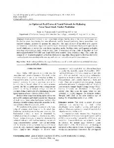
6. Example In this section we report numerical result, using a multi-layer FFNN having one hidden layer with 5 hidden units (neurons) and one linear output unit. The sigmoid activation of each hidden unit is tansig.; the analytic solution 𝑦𝑎 (𝑥) was known in advance. Therefore we test the accuracy of the obtained solutions by computing the deviation: Δ𝑦 (𝑥) = 𝑦𝑡 (𝑥) − 𝑦𝑎 (𝑥) . (11) In order to illustrate the characteristics of the solutions provided by the neural network method, we provide figures displaying the corresponding deviation Δ𝑦(𝑥) both at the few points (training points) that were used for training and at many other points (test points) of the domain of equation. The latter kind of figures are of major importance since they show the interpolation capabilities of the neural solution which to be superior compared to other solution obtained by using other methods. Moreover, we can consider points outside the training interval in order to obtain an estimate of the extrapolation performance of the obtained numerical solution. Example 1. Consider the following 2nd-order TPSBVP: 1 sin (𝑥) = 0, 𝑦 + ( ) 𝑦 + cos (𝑥) + 𝑥 𝑥
𝑥 ∈ [0, 1] ,
(a)
Net.IW{1, 1} 0.2858 0.7572 0.7537 0.3804 0.5678
Weights and bias for trainlm Net.LW{2, 1} 0.0759 0.0540 0.5308 0.7792 0.9340
Net.B{1} 0.1299 0.5688 0.4694 0.0119 0.3371
(b)
𝑑𝑁 (𝑥, 𝑝)⃗ 𝑑2 𝑦𝑡 (𝑥, 𝑝) = 2𝑁 (𝑥, 𝑝) + 2 {(𝑥 − 𝑎) + (𝑥 − 𝑏)} 2 𝑑𝑥 𝑑𝑥 + (𝑥 − 𝑎) (𝑥 − 𝑏)
MSE 2.1859𝑒 − 009 6.6751𝑒 − 009 2.0236𝑒 − 011
(12)
Net.IW{1, 1} 0.4068 0.1126 0.4438 0.3002 0.4014
Weights and bias for trainbfg Net.LW{2, 1} 0.8334 0.4036 0.3902 0.3604 0.1403
Net.B{1} 0.2601 0.0868 0.4294 0.2573 0.2976
(c)
Net.IW{1, 1} 0.1696 0.2788 0.1982 0.1951 0.3268
Weights and bias for trainbr Net.LW{2, 1} 0.8803 0.4711 0.4040 0.1792 0.9689
Net.B{1} 0.4075 0.8445 0.6153 0.3766 0.8772
with BC: 𝑦 (0) = 0, 𝑦(1) = cos(1). The analytic solution is 𝑦𝑎 (𝑥) = cos(𝑥); according to (8) the trial neural form of the solution is taken to be 𝑦𝑡 (𝑥) = cos (1) 𝑥 + 𝑥 (𝑥 − 1) 𝑁 (𝑥, 𝑝) .
(13)
The FFNN trained using a grid of ten equidistant points in [0, 1]. Figure 1 displays the analytic and neural solutions with different training algorithm. The neural results with different types of training algorithm such as Levenberg-Marquardt (trainlm), quasi-Newton (trainbfg), and Bayesian Regulation (trainbr) introduced in Table 1 and its errors given in Table 2, Table 3 gives the performance of the train with epoch and time, and Table 4 gives the weight and bias of the designer network, Ramos in [20] solved this example using 𝐶1 -linearization method and gave the absolute error 4.079613𝑒 − 04; also, Kumar in [21] solved this example by the three-point finite difference technique and gave the absolute error 4.4𝑒 − 05.
ISRN Applied Mathematics
5 Table 5: Analytic and neural solutions of Example 2.
Input 𝑥 0.0 0.1 0.2 0.3 0.4 0.5 0.6 0.7 0.8 0.9 1.0
Analytic solution 𝑦𝑎 (𝑥) 1 1.10517091807565 1.22140275816017 1.34985880757600 1.49182469764127 1.64872127070013 1.82211880039051 2.01375270747048 2.22554092849247 2.45960311115695 2.71828182845905
Out of suggested FFNN 𝑦𝑡 (𝑥) for different training algorithms Trainlm Trainbfg Trainbr 1 0.999999999999781 0.999999991504880 1.10514495970783 1.10517935005948 1.10518327439088 1.22139291634314 1.22140560576571 1.22140301047712 1.34985880757600 1.34985880757533 1.34985789841558 1.49182469764127 1.49182469764283 1.49182590291778 1.64872127070013 1.64872127069896 1.64871934058054 1.82211880039051 1.82211880039100 1.82211668702999 2.01374698451417 2.01375253599035 2.01375577873317 2.22554092849247 2.22554092849241 2.22553872338720 2.45965304884168 2.45961509099396 2.45960396018800 2.71828182845905 2.71828182845889 2.71828168663973 Table 6: Accuracy of solutions for Example 2.
The error 𝐸(𝑥) = |𝑦𝑡 (𝑥) − 𝑦𝑎 (𝑥)| where 𝑦𝑡 (𝑥) computed by the following training algorithm Trainlm Trainbfg trainbr 0 2.19047002758543𝑒 − 13 8.49512027389920𝑒 − 09 2.59583678221542𝑒 − 05 8.43198383004840𝑒 − 06 1.23563152347739𝑒 − 05 9.84181703400644𝑒 − 06 2.84760554247754𝑒 − 06 2.52316951554477𝑒 − 07 0 6.74571509762245𝑒 − 13 9.09160424944489𝑒 − 07 0 1.55675472512939𝑒 − 12 1.20527650837587𝑒 − 06 0 1.16662235427611𝑒 − 12 1.93011959059852𝑒 − 06 2.22044604925031𝑒 − 16 4.86721773995669𝑒 − 13 2.11336051969546𝑒 − 06 5.72295631107167𝑒 − 06 1.71480126542889𝑒 − 07 3.07126269616376𝑒 − 06 0 5.72875080706581𝑒 − 14 2.20510526371953𝑒 − 06 4.99376847331590𝑒 − 05 1.19798370104007𝑒 − 05 8.49031051686211𝑒 − 07 0 1.51878509768721𝑒 − 13 1.41819320731429𝑒 − 07 1.2
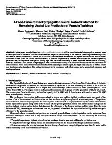
Example 2. Consider the following 2nd-order TPSBVP:
1.1
(1 − 2𝑥) (𝑥 − 1) ]𝑦 − [ ] 𝑦, 𝑥 𝑥
1
𝑥 ∈ [0, 1] .
(14)
0.9 yt
𝑦 = − [
with BC: 𝑦(0) = 1, 𝑦(1) = exp(1) and the analytic solution is 𝑦𝑎 (𝑥) = exp(𝑥); according to (8) the trial neural form of the solution is
0.8 0.7 0.6 0.5
0
0.1
0.2
0.3
0.4
0.5
0.6
0.7
0.8
0.9
1
x
𝑦𝑡 (𝑥) = 1 + (exp (1) − 1) 𝑥 + 𝑥 (𝑥 − 1) 𝑁 (𝑥, 𝑝) .
(15)
The FFNN trained using a grid of ten equidistant points in [0, 1]. Figure 2 displays the analytic and neural solutions with different training algorithms. The neural network results with different types of training algorithm such as trainlm, trainbfg, and trainbr, introduced in Table 5 and its errors given in Table 6, Table 7 gives the performance of the train
ya Trainlm
Trainbfg Trainbr
Figure 1: Analytic and neural solutions of Example 1, using trainbfg, trainbr, and trainlm.
with epoch and time and Table 8 gives the weight and bias of the designer network.
6
ISRN Applied Mathematics 2.8
Table 7: The performance of the train with epoch and time of Example 2.
2.4 2.2 2 yt
TrainFcn Performance of train Epoch Time MSE Trainlm 7.04𝑒 − 33 1902 0:00:30 2.6977𝑒 − 010 Trainbfg 4.00𝑒 − 28 2093 0:01:04 1.8225𝑒 − 011 Trainbr 2.43𝑒 − 12 3481 0:00:56 1.458𝑒 − 011
2.6
1.8 1.6 1.4 1.2
Table 8: Weight and bias of the network for different training algorithm Example 2. (a)
Weights and bias for trainlm Net.LW{2, 1} 0.1626 0.1190 0.4984 0.9597 0.3404
Net.IW{1, 1} 0.7094 0.7547 0.2760 0.6797 0.6551
Net.IW{1, 1} 0.7094 0.7547 0.2760 0.6797 0.6551
Net.B{1} 0.5853 0.2238 0.7513 0.2551 0.5060
Net.B{1} 0.5853 0.2238 0.7513 0.2551 0.5060
(c)
Net.IW{1, 1} 0.9357 0.4579 0.2405 0.7639 0.7593
Weights and bias for trainbr Net.LW{2, 1} 0. 7406 0.7437 0.1059 0.6816 0.4633
0
0.1
0.2
0.3
0.4
0.5
0.6
0.7
0.8
0.9
1
x
(b)
Weights and bias for trainbfg Net.LW{2, 1} 0.1626 0.1190 0.4984 0.9597 0.3404
1 0.8
Net.B{1} 0.2122 0.0985 0.8236 0.1750 0.1636
7. Conclusion From the previous mentioned problems it is clear that the proposed network can be handle effectively TPSBVP and provide accurate approximate solution throughout the whole domain and not only at the training points. As evident from the tables, the results of proposed network are more precise as compared to the method suggested in [20, 21]. In general, the practical results on FFNN show that the Levenberg-Marquardt algorithm (trainlm) will have the fastest convergence, then trainbfg and then Bayesian Regulation (trainbr). However, “trainbr” does not perform well on function approximation problems. The performance of the various algorithms can be affected by the accuracy required of the approximation.
ya Trainlm
Trainbfg Trainbr
Figure 2: Analytic and neural solutions of Example 2 using different training algorithms.
References [1] S. Agatonovic-Kustrin and R. Beresford, “Basic concepts of artificial neural network (ANN) modeling and its application in pharmaceutical research,” Journal of Pharmaceutical and Biomedical Analysis, vol. 22, no. 5, pp. 717–727, 2000. [2] I. E. Lagaris, A. C. Likas, and D. G. Papageorgiou, “Neuralnetwork methods for boundary value problems with irregular boundaries,” IEEE Transactions on Neural Networks, vol. 11, no. 5, pp. 1041–1049, 2000. [3] L. N. M. Tawfiq, Design and training artificial neural networks for solving differential equations [Ph.D. thesis], University of Baghdad, College of Education Ibn-Al-Haitham, 2004. [4] A. Malek and R. Shekari Beidokhti, “Numerical solution for high order differential equations using a hybrid neural network—optimization method,” Applied Mathematics and Computation, vol. 183, no. 1, pp. 260–271, 2006. [5] H. Akca, M. H. Al-Lail, and V. Covachev, “Survey on wavelet transform and application in ODE and wavelet networks,” Advances in Dynamical Systems and Applications, vol. 1, no. 2, pp. 129–162, 2006. [6] K. S. Mc Fall, An artificial neural network method for solving boundary value problems with arbitrary irregular boundaries [Ph.D. thesis], Georgia Institute of Technology, 2006. [7] A. Junaid, M. A. Z. Raja, and I. M. Qureshi, “Evolutionary computing approach for the solution of initial value problems in ordinary differential equations,” World Academy of Science, Engineering and Technology, vol. 55, pp. 578–5581, 2009. [8] J. Abdul Samath, P. S. Kumar, and A. Begum, “Solution of linear electrical circuit problem using neural networks,” International Journal of Computer Applications, vol. 2, no. 1, pp. 6–13, 2010. [9] K. I. Ibraheem and B. M. Khalaf, “Shooting neural networks algorithm for solving boundary value problems in ODEs,” Applications and Applied Mathematics, vol. 6, no. 11, pp. 1927– 1941, 2011. [10] S. A. Hoda I. and H. A. Nagla, “On neural network methods for mixed boundary value problems,” International Journal of Nonlinear Science, vol. 11, no. 3, pp. 312–316, 2011.
ISRN Applied Mathematics [11] K. Majidzadeh, “Inverse problem with respect to domain and artificial neural network algorithm for the solution,” Mathematical Problems in Engineering, vol. 2011, Article ID 145608, 16 pages, 2011. [12] Y. A. Oraibi, Design feed forward neural networks for solving ordinary initial value problem [M.S. thesis], University of Baghdad, College of Education Ibn Al-Haitham, 2011. [13] M. H. Ali, Design fast feed forward neural networks to solve two point boundary value problems [M.S. thesis], University of Baghdad, College of Education Ibn Al-Haitham, 2012. [14] I. Rach˚unkov´a, S. Stanˇek, and M. Tvrd´y, Solvability of Nonlinear Singular Problems for Ordinary Differential Equations, Hindawi Publishing Corporation, New York, USA, 2008. [15] L. F. Shampine, J. Kierzenka, and M. W. Reichelt, “Solving Boundary Value Problems for Ordinary Differential Equations in Matlab with bvp4c,” 2000. [16] H. W. Rasheed, Efficient semi-analytic technique for solving second order singular ordinary boundary value problems [M.S. thesis], University of Baghdad, College of Education Ibn-AlHaitham, 2011. [17] A. I. Galushkin, Neural Networks Theory, Springer, Berlin, Germany, 2007. [18] K. Mehrotra, C. K. Mohan, and S. Ranka, Elements of Artificial Neural Networks, Springer, New York, NY, USA, 1996. [19] A. Ghaffari, H. Abdollahi, M. R. Khoshayand, I. S. Bozchalooi, A. Dadgar, and M. Rafiee-Tehrani, “Performance comparison of neural network training algorithms in modeling of bimodal drug delivery,” International Journal of Pharmaceutics, vol. 327, no. 1-2, pp. 126–138, 2006. [20] J. I. Ramos, “Piecewise quasilinearization techniques for singular boundary-value problems,” Computer Physics Communications, vol. 158, no. 1, pp. 12–25, 2004. [21] M. Kumar, “A three-point finite difference method for a class of singular two-point boundary value problems,” Journal of Computational and Applied Mathematics, vol. 145, no. 1, pp. 89– 97, 2002.
7
Advances in
Operations Research Hindawi Publishing Corporation http://www.hindawi.com
Volume 2014
Advances in
Decision Sciences Hindawi Publishing Corporation http://www.hindawi.com
Volume 2014
Journal of
Applied Mathematics
Algebra
Hindawi Publishing Corporation http://www.hindawi.com
Hindawi Publishing Corporation http://www.hindawi.com
Volume 2014
Journal of
Probability and Statistics Volume 2014
The Scientific World Journal Hindawi Publishing Corporation http://www.hindawi.com
Hindawi Publishing Corporation http://www.hindawi.com
Volume 2014
International Journal of
Differential Equations Hindawi Publishing Corporation http://www.hindawi.com
Volume 2014
Volume 2014
Submit your manuscripts at http://www.hindawi.com International Journal of
Advances in
Combinatorics Hindawi Publishing Corporation http://www.hindawi.com
Mathematical Physics Hindawi Publishing Corporation http://www.hindawi.com
Volume 2014
Journal of
Complex Analysis Hindawi Publishing Corporation http://www.hindawi.com
Volume 2014
International Journal of Mathematics and Mathematical Sciences
Mathematical Problems in Engineering
Journal of
Mathematics Hindawi Publishing Corporation http://www.hindawi.com
Volume 2014
Hindawi Publishing Corporation http://www.hindawi.com
Volume 2014
Volume 2014
Hindawi Publishing Corporation http://www.hindawi.com
Volume 2014
Discrete Mathematics
Journal of
Volume 2014
Hindawi Publishing Corporation http://www.hindawi.com
Discrete Dynamics in Nature and Society
Journal of
Function Spaces Hindawi Publishing Corporation http://www.hindawi.com
Abstract and Applied Analysis
Volume 2014
Hindawi Publishing Corporation http://www.hindawi.com
Volume 2014
Hindawi Publishing Corporation http://www.hindawi.com
Volume 2014
International Journal of
Journal of
Stochastic Analysis
Optimization
Hindawi Publishing Corporation http://www.hindawi.com
Hindawi Publishing Corporation http://www.hindawi.com
Volume 2014
Volume 2014