Dec 7, 2015 - Designer dynamics through chaotic traps: Controlling complex behavior in driven ..... âΩ there exist peaks in the PSD, indicating that it is.
Designer dynamics through chaotic traps: Controlling complex behavior in driven nonlinear systems Shakti N. Menon1 , S. Sridhar1,2 and Sitabhra Sinha1 1
The Institute of Mathematical Sciences, CIT Campus, Taramani, Chennai 600113, India. 2 Department of Chemistry, Brandeis University, Waltham, Massachusetts 02454-9110, USA.
arXiv:1512.02032v1 [nlin.CD] 7 Dec 2015
(Dated: December 8, 2015) Control schemes for dynamical systems typically involve stabilizing unstable periodic orbits. In this paper we introduce a new paradigm of control that involves ‘trapping’ the dynamics arbitrarily close to any desired trajectory. This is achieved by a state-dependent dynamical selection of the input signal applied to the driven nonlinear system. An emergent property of the trapping process is that the signal changes in a chaotic sequence: a manifestation of chaos-induced order. The simplicity of the control scheme makes it easily implementable in experimental systems. PACS numbers: 05.45.Gg,87.19.Hh,87.19.lr,05.45.-a
Nonlinear systems perturbed by external signals exhibit a rich variety of dynamical regimes [1, 2]. Examples include the entrainment of mammalian circadian rhythms to the day-night cycle [3] and the periodic cardiac contractions driven by electrical signals from the sinus node [4, 5]. External signals may also induce pathological conditions, such as when a precisely timed electrical pulse triggers life-threatening arrhythmia in the heart [6] or when aberrant sensory inputs result in reflex epilepsy [7]. A deeper understanding of the dynamical principles governing the response of the system to stimuli can therefore aid in the development of more effective treatment of such disorders. Indeed, externally applied stimuli, such as electromagnetic pulses, have been used to treat several clinical disorders [8, 9]. For example, deep brain stimulation (DBS) [10] has been applied to treat a range of “dynamical diseases” [11], such as Parkinson’s disease [12], major depressive disorder [13] and dystonia [14]. Therapies that involve external electrical [15] or magnetic [8] stimulation are non-invasive, making them an attractive treatment option.
namics, will not only be a theoretical breakthrough, but would also widen the horizon of control in practical applications. Such a method could be used to target instabilities in any physical system driven by external signals, e.g., those observed in magnetically confined plasma [25]. In this paper, we present a novel paradigm for the control of driven dynamical systems by restricting trajectories to a small but finite volume of phase space. This outcome is achieved with minimal information about the state of the system, by switching between a specified set of values of an external signal every time the state crosses a reference threshold. Note that this reference state is quite distinct from the notion of a “target” state (e.g., as in proportional feedback schemes [26]) around which the system is desired to be confined, and consequently the amplitude of the control signal need not be modulated as a function of the difference between the instantaneous and target states. Consider the general setting of a dynamical system F driven by an external signal Ω:
The theory of the control of dynamical systems via tunable signals [16] provides a potential framework for understanding the mechanisms underlying such therapies. The dominant paradigm for the control of nonlinear systems involves applying feedback to perturb an accessible system variable or parameter to stabilize an unstable periodic orbit (UPO) [17, 18]. This approach has been implemented in diverse experimental systems [19– 24]. Practical implementations of such “closed-loop” feedback schemes require significant computational effort as they typically presume detailed knowledge of the dynamical state of the non-linear system and often involve high information processing overhead. A fundamental limitation of such approaches is that the permissible controlled states are intrinsically connected to the specific dynamics of the system. From this perspective, a control scheme designed to maintain the system around an arbitrary state, using minimal information about its dy-
Here Xn is the state of the system at time n, G is the deterministic control function, and the signal Ωn is varied over time in order to impose control. While G could be continuous, we demonstrate that a suitably chosen discrete-valued function, that is characterized by Ω switching between a finite set of values, dynamically creates a trapping region around a desired state of F . On entering the switching-induced “trap”, X is constrained to remain within it and follows a chaotic trajectory, even for regimes where the uncontrolled dynamical system F (Xn , Ωn = Ω) does not display chaos. Furthermore, the sequence of Ωs arising from the deterministic rule G during control is also chaotic. Thus, chaos, which most control schemes try to eliminate, is here an intrinsic feature of the controlled state. This outcome can hence be seen as a manifestation of “chaos-induced order”, analogous to the emergence of order in stochastic systems through the application of noise [27, 28]. We demon-
Xn = F (Xn−1 , Ωn ) , Ωn = G(Xn−1 ) .
(1)
2 strate that a binary-valued function G involving discrete switching between Ωa and Ωb is sufficient to control F . The efficacy of our scheme is highlighted using two dynamical systems driven by external signals. In each case, we show that by starting with a sufficiently large trapping region and strategically altering Ωn , the dynamics can be constrained to any desired phase space volume. While the idea of trapping regions have been used earlier in very specific contexts, such as the modulation of mixing [29], our method creates an adaptable trap that can control the system around an arbitrary state. We first consider a generic model for complex multiperiodic behavior, used to describe the dynamics in systems as diverse as the heart [30] and magnetically confined plasma [25], viz., the circle map (also known as the Chirikov-Taylor map): θn+1 = θn + Ωn − k sin(2 π θn )
(mod 1) .
1 k=1 (a) Ω=0.1 θ n+1 s u 1
s
1
0 1 (b) θ 0
(c)
2
u
2
u
u
s
2
2
s
0
1
k=1 Ω=0.9
θ
θ
10
n
θ
n+1
k=1 a Ω =0.1 b Ω =0.9
1
n+1
1
n
0 1
θ
n
0 1
(d) Ω
n
on
on
off
0 0
(2)
Here, θn is the phase angle describing the state of the system at time n, while Ωn is the corresponding driving frequency. The value of k determines the curvature of the map and thereby, the periodicity of the dynamics. For all simulations reported here, we use values of k ≤ 1, a regime in which the map is invertible and the dynamics are consequently non-chaotic. We control the system by “trapping” the trajectories around a desired value θ0 , an outcome that we achieve by switching between two driving frequencies Ωa and Ωb in a dynamically evolving sequence. The choice of Ω at any instant n depends on the sign of θn − θ0 . Specifically, we set Ωn = Ωa for θn < θ0 and Ωn = Ωb for θn ≥ θ0 . We first demonstrate the trapping scheme for the situation in which the driving frequency, Ω, of the circle map permits the existence of stable and unstable fixed points. Fig. 1 (a) and (b) illustrate the characteristic dynamics of the circle map for two such values of Ω. In each case, the trajectories tend towards the respective stable fixed points. However, switching between these two values of Ω in accordance with our control mechanism results in the effective trapping of trajectories between the unstable fixed points of the constituent maps, as shown in Fig. 1 (c). The implementation of this scheme is not contingent on the existence of fixed points: in the absence of a stable fixed point, the circle map exhibits aperiodic dynamics that can be constrained by switching between values Ωa and Ωb , above and below the original driving frequency [Fig. 1 (d, left)]. Our scheme also allows for the system dynamics to be confined to an extremely small volume of phase space around a desired state. This can be achieved in the situation where the variation of Ωn leads to the emergence of unstable fixed points in the constituent maps [Fig. 1 (c)]. In such cases, the system can be brought arbitrarily close to any desired state by decreasing the absolute value of the difference between the successive values of Ω, while strategically ensuring that the trajectory never leaves the
1
3
n (x 10 )
3
n (x 10 )
3 0
2 0.8
θ
n
0.2 1
(e) Ω
n
0 0
4
n (x 10 )
1 0
4
n (x 10 ) 1
0
4
n (x 10 )
4
FIG. 1: Demonstration of control in the context of the circle map by switching between the two maps (a) F1 : k = 1, Ω = 0.1 and (b) F2 : k = 1, Ω = 0.9, resulting in the controlled situation shown in (c). The switching between Ωa = 0.1 and Ωb = 0.9 “traps” the dynamical state in a region bounded between the unstable fixed points u1 and u2 of the maps F1 and F2 respectively, which is located away from the stable fixed points s1 and s2 of the two maps. (d) Even in the absence of fixed points, control can be achieved (in the sense of reducing the range of values over which θ can dynamically vary) immediately upon turning “on” the switching, i.e., alternating Ωn between a pair of values that characterize two maps (left). It is possible to reduce the trapping region to an arbitrarily small domain by strategically changing Ωn and hence the maps between which switching occurs (right). For both panels, the switching sequence Ωn is shown underneath the time-series of the dynamical variable θ (k = 0.9). (e) Demonstration of the generality of the control method by stabilizing a variety of trajectories through appropriate switching strategies: (left) rectangular wave, (center) sine-like wave and (right) a bursting pattern. For each panel, the switching sequence Ωn is shown underneath the time-series of the dynamical variable θ (k = 0.9).
trapping region [Fig. 1 (d, right)]. The versatility of our control strategy is highlighted by the fact that it can be used to achieve trapping around any arbitrary trajectory θn through appropriate manipulations of Ωn , as illustrated in Fig. 1 (e). In order to characterize the complex dynamics in the trapped region, the Lyapunov exponent, λ, is measured
3
0.6
θn+1
λ
0.49 1
k=0.6
0.2 ∆Ω
0 0.4
u1
u2
θn+1
f(θn)
0 0.2
0.7 (c)
0.3 1
b2
f(θn)
k=0.2 0
b1
(b) k=1.0 0.51
(a)
θn 0.51
0.49
(d)
PSD
100
0 0.3
θn
0.7
∆ Ω=0.001
(e)
∆ Ω=0.1
−2
10
P(L)
0 0
10−6
∆Ω 0.2
0.5 0.1 Frequency
10−8 0
6
L
12
18
FIG. 2: Dynamical properties of the trajectories θn in the trapping region, obtained by implementing the control scheme on the circle map, using a switching sequence Ωn = {Ωa , Ωb }, are illustrated for the case Ωa = 1 + ∆Ω and Ωb = 1 − ∆Ω. (a) Lyapunov exponents for the time series θn , obtained for a range of values of ∆Ω for k = 0.2 (filled upward triangles), k = 0.6 (filled squares) and k = 1 (crosses). (b-c, top) Composite maps for the cases where k = 1 and (b) ∆Ω = 0.01; (c) ∆Ω = 0.25. In (b), b1 and b2 refer to the values of θn+1 at the extremities of the two segments of the composite map, while u1 and u2 are the unstable fixed points. Note that the trapping region in (b) closely resembles the Bernoulli map, while the broken straight lines in (c) are used to highlight the local curvature of the map. (b-c, bottom) Corresponding histogram for the trajectories. (d) Power spectral density for the switching sequence Ωn , obtained over a range of values of ∆Ω for k = 1. (e) Probability that the switching sequence Ωn between the two constituent maps contains a sub-sequence of length L in which it is unchanged. Results are displayed for k = 1, ∆Ω = 0.001 (crosses) and ∆Ω = 0.1 (filled circles). The broken line indicates the transition between the upper and lower branches. The solid line illustrates the characteristic 1/2L behavior expected from a fair coin toss.
for the time series θn . For the situation displayed in Fig. 2, we switch between two maps corresponding to Ωa = 1 − ∆Ω and Ωb = 1 + ∆Ω. Fig. 2 (a) shows that the dynamics in the trapped region is observed to be chaotic for a wide range of k and the control parameter ∆Ω. To understand the origin of chaos in this controlled state, we look at the composite map, i.e., the effective map obtained on application of the control. It comprises two segments separated by a discontinuity that determines the location of the trapping region. For small values of ∆Ω, the trajectories span the domain more or less uniformly, as shown in Fig. 2 (b), a feature that becomes increasingly pronounced as the constituent maps are brought closer together. This can be understood from the fact
that as ∆Ω decreases, the trapping region of the composite map increasingly resembles the Bernoulli map, which produces a dynamical sequence indistinguishable from a fair coin toss [31]. Although the dynamics remain chaotic for larger values of ∆Ω, the trajectories tend to preferentially frequent certain regions, as shown in Fig. 2 (c). This arises due to the increased curvature of the composite map. The transition in behavior is manifested in the corresponding power spectral densities (PSD) of the sequence of driving frequencies, Ωn [Fig. 2 (d)]. For large ∆Ω there exist peaks in the PSD, indicating that it is more likely to obtain a sub-sequence, comprising either Ωa or Ωb , with a specific length. As ∆Ω decreases, subsequences of all lengths L can be observed with the probability expected for the Bernoulli map (∼ 1/2L ). This is confirmed by examining the distribution of sub-sequences of length L for different ∆Ω [Fig. 2 (e)]. For a low value of ∆Ω, the probability of observing large sub-sequences is comparatively high. The likelihood of observing such sequences is very small for higher values of ∆Ω [see lower branch in Fig. 2 (e)] as they occur only when the trajectory is close to one of the unstable fixed points. The observation of chaos in the trapped region can be explained by the fact that the switching control scheme effectively transforms an invertible dynamical system into a non-invertible one. As our method constrains the dynamics arbitrarily close to a desired trajectory in such traps, it suggests a paradigm of control distinct from schemes that involve the stabilization of UPOs. A necessary condition for the creation of a chaotic trap is that the chosen pair of input frequencies tend to drive the trajectories onto opposite branches of the resulting composite map. In general, the values of the two segments of the composite map at the discontinuity provide the maximum bound of the trapping region. In the situation where fixed points exist, the creation of a trap is dependent on the condition that b1 lies below u2 and b2 lies above u1 [Fig 2 (b)]. In this case, the trajectories can neither enter nor leave the trap, although the extent of the trap can itself be dynamically varied, as illustrated earlier in Fig 1 (d). The fact that our scheme constrains the phase space of the dynamics through chaotic switching suggests that it is a mechanism analogous to ‘noiseinduced order’ [32]. In contrast to most feedback methods, which require precise information about the present state of the system, our scheme only depends on whether θn > θ0 or not. One practical consequence of this is that the proposed control scheme is more robust to inaccuracies in the measurement of the dynamical state. Finally, to illustrate the generality of our scheme, we use it to control the dynamics of a realistic model of an excitable biological system, namely the Luo-Rudy (LR) model [33] of an externally stimulated cardiac ventricular cell. The system exhibits a characteristic action potential behavior in the cellular transmembrane potential difference V , i.e., a stimulation above a given threshold leads
(a)
(b)
(ms)
10
V (mv)
n+1
−50 10 −50
20 20 Tn − Dn (ms) 220
0
T (ms)
200
800 (c)
1
n
10
∆ D (ms)
220
D
−1
10
n
T (ms)
241 239 0
400
n 1200 10 (e)
800 a
T = 239 ms b T = 241 ms
(d) −2
10
P(L)
60 Control
−6
10
0
1600
∆ T (ms)
to a large transient excursion from the resting state [34]. The action potential duration (APD) for the nth stimulus, Dn , is measured as the time during which V is above the threshold. The duration of successive excitations depends on whether the medium has been able to sufficiently recover from prior activation. This is reflected in the restitution curve of Fig. 3 (a). Here, under periodic pacing with period T , we observe that the duration of the nth action potential increases with the magnitude of T − Dn−1 . This nonlinear restitution property of cardiac tissue can result in alternans: pathological behavior characterized by alternating long and short action potentials [35]. As seen in Fig. 3 (b, top), rapid stimulation of a single cell can give rise to such a period-2 response in APDs. In order to control this behavior in a single cell, we alter the pacing period by an amount 0 < ∆T ≪ T , such that the period is either T a = T − ∆T or T b = T + ∆T , depending on the sign of Dn − Dn−1 . Varying the pacing periods in this manner maintains a state characterized by near-identical APDs. Note that (i) ∆T is chosen such that pacing exclusively with either T a or T b produces alternans, and that (ii) switching between T a and T b is equivalent to alternating between a pair of values of Ω in the system (1). In Fig. 3 (b, bottom), we show the result of applying the control using ∆T = 4 ms (i.e., stimulating the cell with pacing periods T = 230 ± 4 ms) on the alternans state shown in Fig. 3 (b, top). The system quickly reaches a state where the APDs have almost equal values, indicating the effective termination of alternans [Fig. 3 (c)]. The irregular nature of the switching dynamics is indicated by the wide distribution of lengths L of sub-sequences containing either T a or T b [Fig. 3 (d)]. We quantify the efficacy of the switching control scheme through the standard deviation, σ, of the resulting APD time-series [Fig. 3 (e)]. In situations where the system exhibits alternans, σ is large. When ∆T is increased above a critical value, the value of this measure decreases sharply and control is achieved. As T decreases, the restitution effect becomes more pronounced and the critical value of ∆T necessary for control is larger. The achievement of control is characterized by the transition from a period-2 switching mechanism (alternating at every step between periods T +∆T and T −∆T ) to an aperiodic stimulation sequence [as in Fig. 3 (d)]. Thus, the onset of control is indicated by the emergence of aperiodic or chaotic switching behavior, suggesting a practical method for inferring whether control has been achieved in in vivo experiments. This paper introduces a novel control paradigm with relatively low information processing overhead, utilizing threshold-based switching between a set of input signals. In contrast to conventional feedback control schemes, our method implicitly uses chaos to trap the system dynamics around a desired trajectory of arbitrary complexity. Such a dynamical intervention scheme can have
V (mv)
4
40 20 No control
50
L
150
200
0
220
T (ms)
240
0 σ (ms)
FIG. 3: Dynamics and control in the single-cell Luo-Rudy model. (a) Restitution curve describing the relation between successive action potential durations (APD) obtained using randomly chosen pacing periods, Tn . The trajectory of APD alternans, obtained for a pacing cycle length T = 220 ms (represented by a broken line), is indicated by arrows. (b, top) The time series of voltage V for the case of pacing with a period T = 230 ms, displaying alternating long and short APDs. (b, bottom) Application of switching control to the above system with ∆ T = 4 ms results in almost equal APDs. (c) Difference of successive APDs (∆Dn = Dn+1 − Dn ) (top) as a function of the pacing interval (bottom). The pacing interval corresponding to the initial alternans state is T = 240 ms. Control is applied with ∆T = 1 ms between n = 400 and n = 800. For n > 800, the value of ∆T is decreased gradually to 0.01 ms (bottom), resulting in a marked reduction in alternans (top). (d) Probability that the switching sequence of periods for the case of control with T = 240 ± 1 ms contains sub-sequences of either T a = 239 ms (filled triangles) or T b = 241 ms (filled circles) of length L. (e) Efficacy of the control scheme in reducing alternans, measured through σ, the standard deviation of the APDs, for different values of T and ∆T .
several potential clinical applications, especially in the context of “electroceutical” therapies [36] and treating cardiac arrhythmias [35, 37–39]. A variant of the control scheme has been used to control cardiac alternans in vitro, wherein the frequency of the applied stimulus is determined by the variation in the measured ventricular pressure [40]. The scope of this switching method can be expanded to include control in spatially extended sys-
5 tems, e.g., coupled circle map lattices, making it experimentally realizable in systems like magnetically confined plasma and lasers. We thank V. Balakrishnan, C. K. Chan, N. G. Garnier, G. I. Menon, A. Pumir and V. Sasidevan for helpful discussions. This research was supported in part by the IMSc Complex Systems Project. We thank the HPC facility at IMSc for providing access to “Satpura” which is partly funded by DST (Grant No. SR/NM/NS-44/2009).
[1] A. Pikovsky, M. Rosenblum, and J. Kurths, Synchronization: A universal concept in nonlinear sciences, Cambridge Univ. Press, Cambridge, 2001. [2] L. Glass, Nature (London) 410, 277 (2001). [3] S. M. Reppert and D. R. Weaver, Nature (London) 418, 935 (2002). [4] H. Irisawa, H. F. Brown, and W. Giles, Physiol. Rev. 73, 197 (1993). [5] M. R. Rosen et al., Nat. Rev. Cardiol. 8, 656 (2011). [6] A. T. Winfree, The Geometry of Biological Time, Springer-Verlag, New York, NY, 1980. [7] R. S. Puranam and J. O. McNamara, Nat. Med. 7, 10 (2001). [8] M. S. George, Sci. Am. 289, 66 (2003). [9] S. Luther et al., Nature (London), 475, 235 (2011). [10] M. L. Kringelbach et al., Nat. Rev. Neurosci. 8, 623 (2007). [11] M. C. Mackey and L. Glass, Science 197, 287 (1977);Dynamical disease: Mathematical analysis of human illness, edited by J. B´elair, L. Glass, U. an der Heiden and J. Milton (New York, American Institute of Physics, 1995). [12] B. Rosin et al., Neuron 72, 370 (2011). [13] J. Warner-Schmidt, Nat. Med. 19, 680 (2013). [14] M. Vidailhet et al., New Engl. J. Med. 352, 459 (2005). [15] A. Berenyi, M. Belluscio, D. Mao and G. Buzsaki, Science 337, 735 (2012).
[16] Handbook of Chaos Control, edited by E. Sch¨ oll and H. G, Schuster (Weinheim, Wiley-VCH, 2008). [17] E. Ott, C. Grebogi and J. Yorke, Phys. Rev. Lett. 64, 1196 (1990). [18] S. Boccaletti et al., Phys. Rep. 329, 103 (2000). [19] W. L. Ditto, S. N. Rauseo and M. L. Spano, Phys. Rev. Lett. 65, 3211 (1990). [20] J. Singer, Y-Z. Wang and H. H. Bau, Phys. Rev. Lett. 66, 1123 (1991). [21] R. Roy et al., Phys. Rev. Lett. 68, 1259 (1992). [22] Th. Pierre, G. Bonhomme and A. Atipo, Phys. Rev. Lett. 76, 2290 (1996). [23] A. Garfinkel, M. L. Spano, W. L. Ditto and J. N. Weiss, Science, 257, 1230 (1992). [24] S. Schiff et al., Nature (London) 370, 615 (1994). [25] A. H. Boozer, Rev. Mod. Phys. 76, 1071 (2003) [26] K. J. ˚ Astr¨ om and R. M. Murray, Feedback systems: An introduction for scientists and engineers, Princeton University Press, Princeton, NJ, 2010. [27] H. Yamazaki, T. Yamada and S. Kai, Phys. Rev. Lett. 81, 4112 (1998) [28] T. Shinbrot and F. J. Muzzio, Nature (London) 410, 251 (2001). [29] T. Shinbrot and J. M. Ottino, Phys. Rev. Lett. 71, 843 (1993). [30] L. Glass, Chaos 1, 13 (1991). [31] J. Ford, Phys. Today 36, 40 (1983). [32] F. Sagu´es, J. M. Sancho and J. Garc´ıa-Ojalvo, Rev. Mod. Phys. 79, 829 (2007). [33] C. H. Luo and Y. Rudy, Circ. Res. 68, 1501 (1991). [34] S. Sinha and S. Sridhar, Patterns in Excitable Media, CRC Press, Boca Raton, FL, 2015. [35] K. Hall et al., Phys. Rev. Lett. 78, 4518 (1997). [36] K. Famm, Nature (London) 496, 159 (2013). [37] D. J. Christini et al., Proc. Natl. Acad. Sci. USA 98, 5827 (2001). [38] D. J. Christini et al., Phys. Rev. Lett. 96, 104101 (2006). [39] S. Sinha and S. Sridhar, in Ref. [16], p. 703. [40] S. Sridhar et al., Phys. Rev. E 87, 042712 (2013).