Designing markets for pollution when damages ... - Semantic Scholar

Designing markets for pollution when damages vary across sources : Evidence from the NOx Budget Program Meredith Fowlie* and Nicholas Muller+ *UC Berkeley and NBER + Department

of Economics

Environmental Studies Program Middlebury College email: [email protected] December 17th , 2010

Abstract Designing markets for pollution when damages vary across sources : Evidence from the NOx Budget Program.

Existing and planned emissions trading programs are almost exclusively “emissions-based”, meaning that a permit can be used to o¤set a ton of pollution, regardless of where in the program region the ton is emitted. Designing programs in this way presumes that the health and environmental damages resulting from the permitted emissions are independent of where in the regulated region the emissions occur. A growing body of scienti…c evidence indicates that this is not the case for nitrogen oxides (NOx). When marginal damages from incremental emissions reductions vary signi…cantly across sources, there is the potential to signi…cantly improve the e¢ ciency of permit market outcomes by using facility or region-speci…c marginal damage estimates to determine the terms of permit trading. We estimate the e¢ ciency gains from “damage-based” trading in the context of a major NOx emissions trading program. We …nd that, under the damage-based trading regime, levelized annual abatement costs increase by an estimated $12 M ( i.e. less than 2 percent). However, damages associated with permitted emissions decrease by approximately $62 M annually. The net bene…ts under the policy that incorporates spatially di¤erentiated trading increase by 17%, or almost $50M annually.

Keywords: Market-based Policy, NOx Budget Program, Policy Instrument Choice. JEL Classi…cations: Q54, Q53, Q58 Acknowledgements: Muller wishes to thank the United States Environmental Protection Agency for support under award: EPA-OPEI-NCEE-08-02.

2

Economists have long advocated for market-based approaches to pollution regulation (Montgomery, 1972; Baulmol and Oates, 1988). The past three decades have witnessed large scale experimentation with implementing emissions trading programs in practice. By many measures, this experimentation has been successful. Targeted emissions reductions have been achieved or exceeded, and it is estimated that total abatement costs have been signi…cantly less than what they would have been in the absence of the trading provisions (Carlson et al. 2000; Stavins, 2005) In terms of allocative e¢ ciency, however, most existing cap-and-trade programs fall short of the theoretical ideal. This is because most policies feature spatially uniform emissions permit trading. That is, all sources in an emissions trading program are permitted to trade allowances with all other sources at an e¤ective one-to-one (i.e. ton-for-ton) exchange rate. By equalizing marginal abatement costs across all sources, a one-for-one trading regime will minimize the total abatement costs incurred to meet the emissions cap. However, spatially uniform permit trading will fall short of allocative e¢ ciency when the impact of emissions - the health and environmental harm - varies across regulated sources. Allocative e¢ ciency requires that marginal abatement costs be set equal to marginal damages across all sources (Baumol and Oates, 1987; Montgomery, 1972). For well-mixed pollutants such as CO2 ; abatement cost minimization and allocative e¢ ciency can be achieved simultaneously since the damage caused by emissions does not vary by source (Hoel, Karp, 2000). When a pollutant is "non-uniformly mixed" (i.e. damages from emissions vary across sources), allocative e¢ ciency cannot no longer be achieved by equating marginal abatement costs across sources. Spatial variation in damages across sources thus gives rise to a trade o¤ between minimizing pollution abatement costs and minimizing the damages caused by permitted emissions. This paper investigates these trade o¤s, and the ine¢ ciencies that arise when a non-uniformly mixed pollutant is regulated using a policy that ignores spatial variation in damages from pollution. In an applied exercise, we estimate how outcomes under a landmark emissions trading program, the NOx Budget Program (NBP), would have di¤ered had the program incorporated spatially di¤erentiated trading. Market-based policies can, in theory, be designed to account for spatial variation in damages (Montgomery, 1972; Tietenberg, 1980). Baumol and Oates (1987) use a general equilibrium model

1

to depict optimal pollution taxes in a setting with heterogeneous costs and damages. The optimal tax rate is calibrated to the marginal damage caused by emissions. When damages vary by source, so do the tax rates. Other authors have characterized e¢ cient quantity-based instruments. The key to realizing allocative e¢ ciency is the calibration of permit exchange rates to the ratio of the marginal damage of emissions for each pair of regulated sources (Klaassen, Forsund, Amann 1994; Farrow et al. 2005; Muller and Mendelsohn, 2009). Heterogeneity in pollution damages adds complexity to both the policy design and to the modeling that informs implementation and ex post evaluation. This complexity can increase administrative costs and reduce political palatability. Thus far, regulators have concluded that the bene…ts from spatially di¤erentiated trading do not appear to justify the added complexity. Existing emissions trading programs have adopted ton-for-ton trading of non-uniformly mixed pollution.1 The focus of this paper is the landmark NBP, a large regional emissions trading program a¤ecting large point sources in the Eastern United States. Previous work has documented considerable variation in the per ton damages from NOx emissions (Mauzerall et al., 2005; Tong et al., 2006; Levy et al., 2009; Muller, Tong, Mendelsohn, 2009; Muller and Mendelsohn, 2009). In the design stages of the NBP, policy makers were aware of this heterogeneity and considered imposing restrictions on interregional trading (FR 63(90): 25902). Ultimately, it was decided that the potential bene…ts from this additional complexity would not justify the costs (US EPA, 1998). The program was therefore implemented as a single jurisdiction, spatially uniform trading program in which all emissions are traded on a one-for-one basis. In this paper, with the bene…t of hindsight, we revisit the decision to forego spatially differentiated (or so-called "damage-based") NOx trading in favor of the simpler emissions-based alternatives. The paper begins with a conceptually straightforward model that characterizes the welfare implications of moving from an emissions-based permit trading regime to one that incorporates spatially-di¤erentiated, damage-based permit trading. We …rst consider a stylized, "…rst best" setting that is free of constraints, distortions, or market failures. We then extend the analysis 1

Some programs do incorporate some measures to address spatial variation in damages. In principle, the Acid Rain Program prohibits trades that lead to exceedence of NAAQS. Southern California’s Reclaim program limits NOx permit trading between coastal and inland areas.

2

to accommodate some pre-existing distortions and institutional constraints that are particularly relevant to the policy setting we analyze. Having laid down the theoretical foundations, we turn to the applied policy analysis. In order to estimate the welfare consequences of implementing an emissions-based, versus damage-based, NOx trading program, we simulate …rms’compliance decisions under both the observed and counterfactual policy designs. Our analysis proceeds in four stages. First, source-speci…c marginal damage estimates are generated using a stochastic version of the Air Pollution Emission Experiments and Policy analysis model (APEEP, Muller, Mendelsohn, 2007;2009), AP2. Second, an econometric model of the compliance decisions made by …rms subject to the NBP is used to simulate investment in NOx abatement and the associated ozone season NOx reductions under the existing (i.e. emissions-based) policy and a series of counterfactual (i.e. damage-based) designs (Fowlie, 2010). In the third step, these source-speci…c NOx emissions are processed through AP2 in order to estimate the aggregate health and environmental impacts under each policy scenario. Finally, the analysis is extended to consider the welfare implications of political constraints, pre-existing distortions in the regulated (i.e. electricity) industry, and uncertainty. We de…ne the net bene…ts of a given policy to be equal to the monetized bene…ts associated with the mandated emissions reduction (i.e. the avoided damages) less the costs incurred to reduce NOx emissions. Estimated net-bene…ts increase by 17 percent (or approximately $50 M, annually) when spatial variation in damages is accounted for. This estimate is somewhat conservative in that we assume policy makers would face political constraints that would limit their ability to implement the optimal policy design. If we remove these constraints, cost savings exceed 30 percent. These …ndings are germane to the unfolding debate about market-based regulation of nonuniformly mixed pollutants. As policy makers work to design the next generation of emissions trading programs, this debate has reached a fever pitch. When a spatially uniform cap-and-trade system for regulating mercury emissions was proposed in 2004, it attracted a record number of rulemaking comments. Critics were adamant that emissions trading was inappropriate for a toxic, non-uniformly mixed pollutant like mercury.2 The courts ultimately invalidated the rule. In 2008, 2

Several studies indicated that CAMR would create local hot spots of mercury pollution, disproportionately impacting some communites.

3

a federal district court vacated the Clean Air Interstate Rule and the associated regional NOx trading program, in large part due to policy’s failure to adequately accommodate spatial variation in damages.3 The paper also contributes to a growing literature that compares spatially di¤erentiated and spatially uniform emissions trading in a variety of policy contexts.4 Most relevant to this study is work that has been done to analyze spatially di¤erentiated NOx trading in the Eastern United States. This small literature is comprised of ex ante analyses of zonal trading regimes (i.e. market designs that limit or prohibit trading between multi-state trading zones) (ICF Kaiser, 1996; Krupnick et al. 2000; US EPA, 1998). In general, researchers have found the di¤erences in damages across multi-state trading zones to be relatively small. Consequently, it has been estimated that of the welfare gains from spatially di¤erentiated NOx permit trading are negligible. Our …ndings contradict this earlier work. To understand why, it is instructive to highlight two distinguishing features of this study. First, we use a detailed integrated assessment model to estimate source-speci…c marginal damages. We …nd signi…cant variation in these damages; almost half of this variation occurring within (versus between) state. This suggests that multi-state trading zones are a very blunt instrument to capture spatial variation in NOx emissions damages. Second, in all previous work, emissions market outcomes are simulated using a deterministic, cost-minimization algorithms. Krupnick et al. (2000) acknowledge a limitation of this approach, noting that they can make "no claim that optimizations of the kinds described here re‡ect emissions trading or other particular policies". These optimization models fail to capture salient features of the real world decision processes that drive emissions abatement decisions, and thus market outcomes. In contrast, in our ex post analysis, we are able to use an econometric model to estimate the compliance choices that these plant managers most likely would have made had the NOx emissions market been designed to re‡ect spatial heterogeneity in marginal damages from pollution. http://www.ens-newswire.com/ens/feb2005/2005-02-07-10.html 3 The court found that the CAIR regulation "does not prohibit polluting sources within an upwind state from preventing attainment of National ambient air quality standards in downwind states."State of North Carolina v. Environmental Protection Agency, No. 05-1244, slip op. (2008), District of Columbia Court of Appeals. 4 Policies analyzed in prior work include spatially di¤erentiated groundwater permit trading in Nebraska (Kuwayama and Brozovic, 2010), particulate matter trading in Santiago Chile (O’Ryan, 2000) and the monumental U.S. Acid Rain Program ((Kete, 1992; Muller and Mendelsohn, 2009; Chupp, Banzhaf, 2010)

4

The paper proceeds as follows. Section 1 introduces the theoretical framework and derives some basic theoretical results. Section 2 provides background on the NOx Budget Program. Section 3 introduces the applied analysis and presents the results. Section 4 concludes.

1

Welfare implications of spatially di¤erentiated emissions trading

In this section, we introduce the theoretical foundations underlying our applied policy analysis. A simple theory model is used to characterize the welfare implications of moving from an emissionsbased permit trading regime to one that incorporates spatially-di¤erentiated permit trading. We …rst consider a stylized, "…rst best" setting. We then extend the analysis to accommodate some pre-existing distortions and institutional constraints that could potentially a¤ect outcomes in the NOx emissions trading program we analyze.

1.1

Theory model

Consider an industry comprised of N …rms producing a homogenous good: Industrial production generates harmful pollution. This pollution is non-uniformly mixed, meaning that the extent of the damage caused by emissions depends not only on the level of emissions, but also how the permitted emissions are distributed across sources.5 Let Ei0 denote the baseline emissions at …rm i; this is the level of emissions we would observe absent any regulatory constraint. The …rm can reduce emissions below Ei by investing in abatement ai . Firm-level emissions are thus Ei = Ei0 of emissions: Ci (Ei ). We assume that Ci0 (Ei )

ai :We de…ne abatement cost functions in terms 0; C"i (Ei )

0: We accommodate heterogeneity in

abatement costs by allowing the parameters of the abatement function to vary across …rms. Damages from emissions also vary across facilities. We de…ne …rm-speci…c damage functions Di (Ei ): We make several simplifying assumptions regarding the structure of these damages. First, N X we assume that aggregate damages D are additively separable: D = Di (Ei ): Second, we i=1

assume …rm-level damages are linear in emissions: Di (Ei ) = ki + 5

i Ei .

Finally, we assume the the

In this analysis, we will focus exclusively on the spatial heterogeneity in damages. See Joskow, Martin and Ellerman (CITE) for an analysis of the implications of temporal variation in damages.

5

parameters of the …rm-speci…c damage functions are known with certainty. In subsequent sections we investigate the implications of relaxing these assumptions. The policy designs we consider are, in many respects, standard "cap-and-trade" programs. An emissions cap E limits the total quantity of permitted emissions. A corresponding number of tradable permits are allocated. We assume that emissions permits are allocated either by auction or a gratis using some allocation rule that does not depend on production decisions going forward (such as grandfathering). Any free allocation of permits to …rm i is represented by the initial allocation Ai . All of the policy designs we consider are "emissions equivalent", meaning that emissions constraint E is held constant across the policy scenarios. Although we are ultimately concerned about limiting the damages associated with pollution exposure, in all existing and planned cap-and-trade programs, the cap is de…ned in terms of emissions. This is presumably because imposing a cap on emissions is relatively simple and easy to communicate. To comply with the regulation, …rms must hold permits to o¤set their uncontrolled emissions. We assume that facilities comply with the regulation either by holding emissions permits, investing in emissions abatement, or some combination of these two strategies. We rule out reduction in output as a compliance strategy and assume that …rm-level production and aggregate output are exogenously determined and independent of the environmental compliance choice. This assumption is appropriate for the policy context we consider.6 We use the following total social cost measure (T SC) to evaluate equilibrium outcomes under the alternative policy scenarios: 6

Our analysis focuses exclusively on coal plants who account for the vast majority of NOx emissions regulated under the NBP. These coal plants are are typically inframarginal due to their relatively low fuel operating costs. The introduction of the cap-and-trade program therefore reduced pro…t margins but not capacity factors at these units (Fowlie, 2010). Price-setting units (typically natural gas or oil-fueled plants) represent a very small fraction of the NOx emissions regulated under the NBP and tend to have much lower uncontrolled NOx emissions rates. Whereas the average pre-retro…t NOx emissions rate among coal plants exceeded 5.5 lbs/MWh, average NOx emissions rates among marginal electricity producers are estimated to range between 0.3 to 2.2 lbs NOx/MWh (NEISO, 2006; Keith et al., 2003). If compliance costs incurred at marginal units were passed directly through to consumers, retail electricity prices would be unlikely to increase by more than one percent on average. Given the small magnitude of this price change, and given the inelasticity of electricity demand, we make the simplifying assumption that total production levels are una¤ected by the introduction of the NOx emissions trading program.

6

T SC =

N X

(Di (Ei ) + Ci (ei ))

(1)

i=1

Any policy-induced change in social welfare will be captured by changes in (1) (because production and consumption levels are exogenous):

1.2

First-best Outcome.

To keep the analytics simple and intuitive, we consider a case with only two price taking …rms. Producers are denoted h and l to indicate high and low damage areas respectively. For each …rm we de…ne a marginal damage parameter

i

= Di0 (Ei ) which captures the damages (measured in

dollars) caused by an incremental change in Ei : We assume,

l


0).

Figure 2 helps to illustrate the qualitative implications of an emissions cap that is too stringent. This …gure is identical to Figure 1, except that we now assume smaller damage parameters for each source, such that E < E ( ; ). By (11), marginal abatement costs are set equal to the product of the permit price and the damage-based compliance ratio: 8

See Appendix 2 for the derivation.

15

Ci0 (Eid ) = This implies that Ci0 (Eid ) >

i

i

=

( i

l 2h

+ ( h

h 2l 2l

+

2 l 2h )

2h 2l )

>

i

(25)

for i = l; h:

In Figure 2, industry-wide abatement costs under damage-based permit trading exceed costs under emissions-based trading by an amount equal to the area of the shaded triangle. The shaded rectangle represents the bene…ts (in the form of avoided emissions damages) associated with spatially di¤erentiated trading using the new damage parameters. In this case, the bene…ts from spatially di¤erentiated permit trading no longer exceed the costs such that the emissions-based trading regime now welfare dominates the damage-based regime. In contrast, if

> 0 and the cap

is not su¢ ciently stringent; the welfare gains from spatially-di¤erentiated trading increase relative to the benchmark …rst-best case.

1.6.3

Pre-existing abatement cost distortions in the product market

Pre-existing distortions in the product market can also a¤ect the e¢ ciency properties of permit market outcomes. For example, the electricity generating units in the NOx emissions trading program face di¤erent economic regulatory incentives in their respective electricity markets. Some forms of electricity market regulation have the potential to distort environmental compliance choices (Fowlie, 2010). Figure 3 helps to illustrate a case in point. Here we assume that the high damage …rm is subject to economic regulation that subsidizes investment in emissions abatement. This may occur in regulated electricity markets when producers are guaranteed to earn a positive rate of return on capital investments in pollution abatement equipment. The marginal abatement cost schedule denoted MACh re‡ects the true abatement costs, whereas the abatement cost curve denoted MAC’h re‡ects the abatement costs as perceived by the …rm. This regulatory distortion moves the equilibrium outcome under emissions-based trading closer to the optimum. In the damage-based trading regime, marginal abatement costs exceed damages at the high damage …rm, whereas the reverse is true at the low damage …rm. As a result, these pre-existing regulatory incentives distort environmental 16

compliance incentives in a way that reduces the net bene…ts from spatially di¤erentiated permit trading are reduced. Of course, pre-existing distortions can work in the other direction if they e¤ectively reduce costs as perceived by relatively low damage sources.

1.6.4

Damage function mispeci…cation

In this working paper, we will assume that the e¤ect of an incremental change in emissions at source i on health and environmental outcomes can be adequately captured by the scalar

i.

More precisely,

we assume that aggregate damages D are linear and additively separable in terms of source-speci…c emissions Ei . These damage parameters, and corresponding trading ratios, are estimated once; they are not permitted to adjust as investments are made in NOx control equipment and emissions rates of other sources are reduced. In future work, we will evaluate the plausibility of the assumptions we make about the damage function. In particular, we will investigate the extent to which periodically updating trading ratios could improve the e¢ ciency of damage-based permit trading.

1.6.5

Risk and uncertainty in damage measures

Another maintained assumption in this working paper is that the damage parameters

are known

with certainty. In fact, estimation of these parameters is predicated upon a complex series of assumptions and approximations. For expositional clarity, we de…ne three main di¤erent sources of uncertainty that can complicate the estimation of these marginal damage parameters. The …rst is air quality modeling uncertainty. In order to estimate source-speci…c damage parameters, we must …rst model how changes in emissions levels at one point in the airshed a¤ects pollution concentrations at all other points in the airshed. The pollution formation, transport, and deposition processes that determine how a change in emissions at one location a¤ects pollution concentrations and exposure at other points in space and time are complex. This complexity begets uncertainty about how these processes should best be represented in a modeling framework. 17

The second source of variability stems from the data used to estimate these models. Pollutant formation and transport can be a highly stochastic process that depends fundamentally on weather patterns, meteorological conditions, pre-existing precursor concentrations, and other hardto-predict phenomena. The third source of uncertainty is introduced when pollution concentrations are converted into monetized damages. This requires a series of additional assumptions about how changes in pollution concentrations at a given location a¤ect health and environmental outcomes, and about how much these outcomes are worth. In this working paper, we will use point estimates of the source-speci…c marginal damage coef…cients to de…ne the terms of trade. In future work. we will explore the implications of the three aforementioned sources of uncertainty surrounding these estimates.

2

Empirical application: the NOx Budget Program

The NOx Budget Program (NBP) is an emissions trading program that limits emissions of NOx from large stationary sources in nineteen eastern states. The NBP was primarily designed to help Northeastern and Mid-Atlantic states attain Federal ozone standards. Prior to the introduction of this program, large point sources in the region were subject to a prescriptive standard that required the installation of low NOx burners. These standards proved insu¢ cient. When the NBP was promulgated, signi…cant portions of the Northeast, Mid-Atlantic, and parts of the Midwest were failing to meet Federal standards (Ozone Transport Assessment Group (OTAG), 1997). Although the precise contribution of individual sources to the non-attainment problems and associated damages in this region was di¢ cult to estimate precisely, there was plenty of evidence to suggest that marginal damages varied signi…cantly across sources. The EPA received over 50 responses when, during the planning stages of the NOx SIP Call, it solicited comments on whether the program should incorporate trading ratios or other restrictions on interregional trading in order to re‡ect the signi…cant di¤erential e¤ects of NOx emissions across states(FR 63(90): 25902). Most commentors supported unrestricted trading and expressed concerns that “discounts or other 18

adjustments or restrictions would unnecessarily complicate the trading program, and therefore reduce its e¤ectiveness”(FR 63(207): 57460). These comments, together with a simulation exercise which indicated that imposing spatial constraints on trading would not signi…cantly a¤ect the location of emissions (US EPA, 1998a), led regulators to design a single jurisdiction trading program in which all emissions are traded on a one-for-one basis. In our analysis, we use data collected from 632 coal-…red generating units that are regulated under the NOx Budget Program. Although gas- and oil-…red generators and other industrial point sources are also included in the NBP, these coal-…red units represent over 90 percent of the NOx emissions regulated under the program and at least 94 percent of the NOx emissions reductions over the …rst …ve years (U.S. EPA, 2005; US E.P.A. 2008). Table 1 presents summary statistics for unit-level operating characteristics that signi…cantly determine NOx emissions levels. To construct this table, units are classi…ed as either "high damage" (above average) or "low damage" (below average) units. This damage classi…cation is described in detail in section 3.1. Overall, these unit-level characteristics are very similarly distributed similarly across the two groups.

3

Ex post analysis of spatially di¤erentiated NOx trading

The primary objective of our applied analysis is to examine the implications of spatially di¤erentiated NOx trading in a landmark emissions trading program. Section 1 laid the conceptual foundations for this exercise. The theoretical model also helps to highlight the essential inputs and outputs of our analysis. Inputs include the source-speci…c demand parameters , the unit speci…c abatement cost schedules Ci (Ei ); and the decision rule that dictates how …rms in an emissions trading program make their abatement investment decisions. Key outputs include the relative impact of spatially di¤erentiated NOx trading on aggregate abatement costs, analogous to C x ( ; )

C e ( ; ) in (19);

and the relative impact of spatially di¤erentiated NOx trading on aggregate damages, analogous to Dx ( ; )

De ( ; ) in (20). In what follows, we describe these inputs and outputs in detail.

19

3.1

Source-speci…c damage parameters

NOx emissions a¤ect health and environmental outcomes through two main pathways: ozone formation and particulate matter formation.9 Speci…cally, emitted NOx interacts with ambient ammonia to form ammonium nitrate, a constituent of ambient PM2:5 . And NOx also forms tropospheric O3 through a series of chemical reactions (Seinfeld, Pandis, 1998). Both PM2:5 and O3 are criteria air pollutants regulated under Title I of the Clean Air Act. As such, exposures to these two pollutants have been shown to have a number of adverse e¤ects on human health and welfare. Prior research has shown that the majority of damages due to exposures to both PM2:5 and O3 are premature mortalities and increased rates of illness (USEPA, 1999; Muller and Mendelsohn, 2007;2009). Exposure to elevated concentrations of either pollutant has been linked to signi…cant human health and ecosystem damages (see, for example, Brunekreef and Holgate, 2002; WHO, 2003). The extent to which NOx emissions react with precursors to form ozone or particulate matter depends upon prevailing meteorological conditions, pre-existing precursor emissions concentrations, and other factors that vary across time and space. Furthermore, the health impacts associated with a change in ozone and/or particulate matter at a particular location will depend on the human and non-human populations at that location. In sum, the damage caused by a given quantity of NOx emissions will depend on the spatial distribution of the emissions.10 The source-speci…c

i

parameters capture how an incremental change in NOx emissions at

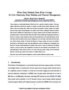
source i a¤ects damages across the airshed through changing concentrations of (and thus exposure to) ozone and particulate matter. In order to connect emissions of NOx to concentrations of both PM2:5 and O3 and to the resultant physical impacts and damages, this paper employs AP2, a stochastic version of the APEEP model which has been used in prior research (Muller and Mendelsohn, 2007;2009). Figure 9 provides a diagram of the AP2 model. AP2 is a standard integrated assessment model in its overall structure. The model is comprised of six modules; emissions, air quality modeling, concentrations, exposures, physical e¤ects, and monetary damages. The emissions data used in 9

NOx emissions also contribute to acid rain in some mountain regions, and exacerbate eutrophication problems. The NOx Budget Program does not explicitly account for spatial variation in marginal damages from emissions; a permit can be used to o¤set a unit of NOx emissions, regardless of where in the program region the unit is emitted. 10

20

AP2 is provided by the USEPA’s National Emission Inventory for 2005 (US EPA, 2009). These data encompass emissions of NOx ; PM2:5 , sulfur dioxide (SO2 ), volatile organic compounds (VOCs), and ammonia (NH3 ). AP2 attributes these data to both the appropriate source location and source type. Speci…cally, AP2 models emissions from 656 individual point sources (mostly large EGUs). Emissions from the remaining point sources are decomposed according to height of emissions and the county in which the source is located. For ground-level emissions (these are produced by cars, residences, and small commercial facilities) AP2 attributes these discharges to the county in which they are reported (by USEPA) to occur. The approach to air quality modeling used in AP2 relies on the Gaussian Plume model (Turner, 1994). This tack uses a reduced form statistical model to capture the processes that connect emissions to concentrations. The predictions from the AP2 model have been tested against the predictions made by a more advanced air quality model (see Muller and Mendelsohn, 2007). The agreement between the county-level surfaces produced by the two models is quite strong. AP2 then connects ambient concentrations to physical impacts using peer-reviewed dose-response functions. In order to model impacts of exposure to PM2:5 on adult mortality rates, this analysis uses the …ndings reported in Pope et al., (2002). The impact of PM2:5 exposure on infant mortality rates is modeled using the results from Woodru¤ et al., (2006). For O3 , we use the …ndings from Bell et al., (2004). In addition, this analysis includes the impact of exposure to PM2:5 on incidence rates of chronic bronchitis (Abbey et al., 1993). The …nal modeling step in connecting emissions to damages is expressing the physical e¤ects predicted by the dose-response functions in monetary terms. To do this, we rely on valuation methodologies used in the prior literature. In order to value the risk of premature mortalities due to pollution exposure, we employ the Value of a Statistical Life (VSL) method. (See Viscusi and Aldy, 2004 for a summary of this literature.) In particular, we employ a VSL of approximately $6 million; this value, which is used by USEPA, results from a meta-analysis of nearly 30 studies that compute VSLs. Further, each case of chronic bronchitis is valued at approximately $300 thousand which is also the value used by USEPA. The marginal ($/ton) damage for NOx for the 632 coal-…red electricity generating units are estimated using the marginal damage algorithm developed in Muller and Mendelsohn (2007;2009).

21

This algorithm includes the following steps. First, baseline emissions are constructed from detailed emissions data collected by the US EPA in the years immediately preceding the introduction of the NOx Budget Program. These emissions re‡ect the NOx controls required for all sources in non-attainment areas. AP2 computes total national damages associated with these baseline levels of NOx emissions: Next, one ton of NOx is added to baseline emissions at a particular EGU. AP2 is the re-run. Concentrations, exposures, physical e¤ects, and damages are recomputed. Since the only di¤erence between the baseline run and the "add-one-ton" run is the additional ton of NOx , the change in damages is strictly attributable to the added ton. This design is then repeated over all of the EGUs encompassed by the NBP.11 Figure 4 summarizes the unit speci…c point estimates of marginal damages from NOx emissions. The average parameter value is $2180/ton of NOx emitted during ozone season. These parameters vary signi…cantly across the sources in the program. Notably, a signi…cant amount of this variation (approximately 45 percent) occurs within (versus between) states. This suggests that a zonal trading regime that employs state-level trading ratios (and permits one-for-one trading within states) would be a fairly blunt policy instrument. For …ve of the 632 units in our data, we …nd that the estimated damage parameters are negative. This suggests that a decrease in NOx emissions at these sources leads to increased overall damages. This seemingly counterintuitive result is driven by the complex, non-linear photochemical reactions that transform NOx and VOCs into ozone. Daily ozone concentrations are non-linear and monotonic functions of NOx and the ratio of volatile organic compounds (VOCs) and NOx. At su¢ ciently low ratios, the conversion of NOx to ozone is limited by the availability of VOCs. In these VOC limited conditions, reductions of NOx can increase peak ozone levels until the system transitions out of a VOC-limited state. With these unit-speci…c damage parameter estimates in hand, it is straightforward to construct the compliance ratios. For each source, we divide the source-speci…c damage measure

i

with the

mean value : Figure 5 plots the compliance ratios we will use in our primary damage-based policy counterfactual as a function of the estimated damage parameters. Relatively "high damage" units 11

In this working paper, all of our analysis is based on the point estimates of these marginal damage parameters. Future work will investigate the implications of the uncertainty surrounding these estimates.

22

are required to hold ri > 1 permit per ton of emissions under the spatially-di¤erentiated trading counterfactual, whereas relatively "low damage" units are required to hold ri < 1 permit per ton. Note that there are no negative trading ratios. We assume that incentivize pollution at facilities with negative damage parameter estimates would be politically unpopular. We thus assign the …ve units with negative marginal damage estimates a compliance ratio of zero, equivalent to dropping them from the program under the damage-based regime.

3.2

NOx abatement costs

The NBP mandated a dramatic reduction in average NOx emissions rates.12 In the period between when the rule was upheld by the US Court of Appeals (March 2000) and the deadline for full compliance (May 2004), …rms had to make costly decisions about how to comply with this new regulation. To comply, …rms can do one or more of the following: purchase permits to o¤set emissions exceeding their allocation, install one or more NOx control technologies, or reduce production at dirtier plants during ozone season. Two factors that are likely to signi…cantly in‡uence a manager’s choice of environmental compliance strategy are the up-front capital costs and anticipated variable compliance costs (i.e. compliance costs incurred per unit of electricity produced). The capital costs, variable operating costs, and emissions reduction e¢ ciencies associated with di¤erent compliance alternatives vary signi…cantly, both across NOx control technologies and across generating units with di¤erent technical characteristics. The speci…c NOx control options available to a given unit also vary across units of di¤erent vintages and boiler types. Compliance options that incorporate Selective Catalytic Reduction (SCR) technology can reduce emissions by up to ninety percent. NOx emissions rates can be reduced by thirty-…ve percent through the adoption of Selective Non-Catalytic Reduction Technology (SNCR). Pre-combustion control technologies such as low NOx burners (LNB) or combustion modi…cations (CM) can reduce emissions by …fteen to …fty percent, depending on a boiler’s technical speci…cations and operating characteristics. 12 Pre-retro…t emissions rates at a¤ected coal plants were, on average, three and a half times higher than the emissions rate on which the aggregate cap was based (0.15 lbs NOx/mmbtu).

23

We do not directly observe the variable compliance costs and …xed capital costs or the post-retro…t emissions rates that plant managers anticipated when making their decisions. We can, however, generate detailed, unit-speci…c engineering estimates of these variables using detailed unit-level and plant-level data. In the late 1990s, to help generators prepare to comply with marketbased NOx regulations, the Electric Power Research Institute13 developed software to generate cost estimates for all major NOx control options available to coal-…red boilers, conditional on unit and plant level characteristics. The software has been used not only by plant managers, but also by regulators to evaluate proposed compliance costs for the utilities they regulate (Himes, 2004; Musatti, 2004; Srivastava, 2004). This software was used to generate the unit-speci…c cost estimates used in this analysis (EPRI, 1999b). This cost estimation exercise is described in detail in Fowlie (2010). Table 2 presents means and standard deviations of the capital and variable costs (estimated at the unit level) for the most commonly adopted NOx control technologies. On average, capital costs are somewhat higher among units located in low damage areas.

3.3

Firm-level compliance decisions

In order to simulate …rms’ response to di¤erent emissions trading program designs, we use an empirical model developed by Fowlie (2010). The basic structure of this discrete choice model is as follows. The manager of unit i (i = 1::632) faces a choice among Ji compliance strategy alternatives (indexed by j; j = 1:::Ji ). Plant managers are assumed to choose the compliance strategy that minimizes the unobserved latent value Cij . The deterministic component of Cij is a weighted sum of expected annual compliance costs vij , the expected capital costs Kij associated with initial retro…t and technology installation, and a constant term

Cij where vij

=

j

+

v i vij

+

j

that varies across technology types :

K i Kij

+

KA

Kij Ageij + "ij ;

(26)

= (Vij + ri mij )Qi

13 The Electric Power Research Institute (EPRI) is an organization that was created and is funded by public and private electric utilities to conduct electricity industry relevant R&D.

24

An interaction term between capital costs and demeaned plant age is included in the model because older plants can be expected to weigh capital costs more heavily as they have less time to recover these costs. The variable cost (per kWh) of operating the control technology is Vij . The variable cost associated with o¤setting emissions with permits is equal to the product of the permit price , the compliance ratio ri and the post-retro…t emissions rate mij . In the observed emissions-based policy regime, ri = 1 for all units. Expected average annual compliance costs are obtained by multiplying estimated per kWh variable costs by expected seasonal production Qi . We maintain the assumption that expected seasonal electricity production (Qn ) is independent of the compliance strategy being evaluated.14 With some additional assumptions, this model can be implemented empirically as a randomcoe¢ cients logit (RCL) model. More speci…cally, the "nj are assumed to be iid extreme value and independent of the covariates in the model. The variable cost coe¢ cient ( K

cost coe¢ cient (

v

) and the capital

) are allowed to vary randomly in the population according to a bivariate

normal distribution, thereby accommodating any unobserved heterogeneity in responses to changes in compliance costs.15 The model is estimated separately for units serving restructured wholesale electricity markets versus publicly owned units and units subject to cost-of-service regulation (see Fowlie (2010)). The estimated parameters of the random coe¢ cient distributions are then combined with information about observed choices in order to make inferences about where in the population distribution a particular plant manager most likely lies. A more detailed description of the model speci…cation, estimation results, and the derivation of manager-speci…c coe¢ cient distributions can be found in Fowlie (2010). We use the RCL coe¢ cient estimates, together with the implied manager-speci…c distributions of the

K

and

v

parameters, to simulate outcomes under the observed emissions-based policy

design and the counterfactual, damage-based designs. The simulations proceed as follows: 14

Anecdotal evidence suggests that managers used past summer production levels to estimate future production (EPRI, 1999a). We adopt this approach and use the historical average of a unit’s past summer production levels (Qn ) to proxy for expected ozone season production. 15 It is common in the literature to assume that cost coe¢ cients are lognormally distributed, so as to ensure the a priori expected negative domain for the distribution (with costs entering the model as negative numbers). Model speci…cations that assumed a log-normal distribution for cost coe¢ cient failed to converge.

25

1. A policy scenario (i.e. the permit market design to be analyzed) is de…ned in terms of the compliance ratios vector r and the emissions cap E. 2. For each manager, for each random parameter, Z random draws from the appropriate managerspeci…c density are taken. Let bmz represent the z th draw from the distribution of coe¢ cients associated with manager m. 3. Beginning with repetition z = 1, simulation of the market clearing permit price

z

and

emissions begins by setting the permit price equal to 0. 4. For each unit, choice probabilities are approximated for all available compliance choices conditional on the prevailing permit price , the coe¢ cient vector bmz , the trading ratio vector r and the unit-speci…c choice set characteristics. Managers are assumed to choose the compliance strategy with the highest estimated probability. 5. Ozone season emissions (measured in lbs of NOx) and engineering estimates of compliance costs associated with the predicted choices are calculated and summed across units. 6. If the total quantity of emissions equals the cap,

is the equilibrium price and the simula-

tion stops. If the total quantity of emissions exceeds (is less than) the cap,

is increased

(decreased) by $0.01. 7. Steps 4-6 are repeated until an equilibrium is reached.16 8. Steps 3-7 are repeated Z times for each policy scenario. Under the baseline policy scenario, r = 1 for all units and the emissions cap E is set equal to the emissions implied by the observed compliance choices. To simulate outcomes under damage based trading, the estimated, source speci…c compliance ratios are used to de…ne the terms of compliance. This e¤ectively increases (decreases) the costs of o¤setting uncontrolled emissions using permits for a relatively high (low) damage …rm. 16

If this iterative procedure arrives at a point where it is vascillating around the cap, the price that delivers the quantity of emissions just below the cap is chosen to be the equilibrium price. Equilibrium emissions are calculated and the simulation stops.

26

This approach assumes that the structure of these …rm-level compliance decisions, and in particular, the relative weighting of capital costs and variable operating costs, would not change if the terms of compliance were damage-based versus emissions-based. We believe this to be a very reasonable assumption. Once di¤erences in variable operating costs across the two regimes are accounted for, we see no reason why a plant manager would take a fundamentally di¤erent approach to compliance. Figures 6 and 7 o¤er a graphical summary of our simulation results. Each point in these scatterplots represents a di¤erent electricity generating unit. The horizontal axis measures the source-speci…c damage parameters we introduced in section 3.1. These are adjusted slightly; the …ve negative marginal damage estimates are set to zero. The horizontal axis in Figure 6 measures the percentage change in unit-level emissions, moving from spatially uniform trading to the spatially di¤erentiated trading regime. Intuitively, units with relatively low (high) damage parameters will increase (reduce) emissions under a damage-based regime. Note that the emissions levels at many units are una¤ected by the policy design change. Given the discrete nature of the NOx abatement choice, a unit’s cost minimizing choice of emissions abatement (and thus emissions) need not be a¤ected by a change in the cost of holding permits to o¤set emissions. Figure 8 conducts a similar exercise using data on simulated levelized annual abatement costs. The horizontal axis measures the di¤erence in simulated levelized annual abatement costs across the emissions equivalent, emissions-based and damage-based trading regimes. Intuitively, investment in abatement is lower (higher) in the spatially di¤erentiated trading regime at the units with relatively low (high) damage parameters. Tables 3 and 4 summarize these simulation results in more detail. Table 3 summarizes the unit-level simulation results. For each unit, simulated emissions and abatement costs are summed within policy scenario across 50 repetitions. Table 3 summarizes the unit-speci…c averages. Average unit-level emissions reductions are approximately the same across these emissions equivalent policy designs. Slight di¤erences (which disappear when numbers are expressed in millions of lbs) are due to the fact that the emissions cap is rarely met exactly. Note that whereas the average change in emissions across regimes is close zero (because emissions increases at relatively low damage …rms

27

balance out the emissions decreases at relatively high damage …rms), levelized annual abatement costs increase by $0.02 M on average. Table 4 reports simulation results aggregated by damage category and averaged across the Z simulation repetitions. The high damage category includes the 241 units with damage parameters that exceed $2180/ton. The low damage category includes the remaining 391 units with below average damage parameters. Transitioning from spatially uniform to spatially di¤erentiated trading shifts approximately 6% of the permitted emissions (or 72 M lbs NOx/year) away from these high damage facilities and into regions where the emissions do less damage. This shift will unambiguously lower the damages caused by the permitted emissions. But this reallocation comes at a cost. As emissions levels increase among low damage units, abatement costs dall by approximately $50M/year in levelized annual costs. However, abatement costs in the high damage area increase by approximately $63 M per year. In sum, estimated levelized annual abatement costs under spatially di¤erentiated trading are approximately $12 higher than simulated abatement costs under the observed, spatially uniform trading regime.

3.4

Estimating damages cause by permitted emissions

AP2 is also used to quantify the change in damages due to the various policy scenarios explored in the study. In this context, rather than systematically perturbing NOx emissions one source at-a-time, NOx emissions change simultaneously at many of the regulated EGUs in response to the di¤erent modeled policies. Here, a vector of NOx emissions corresponding to the output from the econometric cost model is processed by AP2. The resulting damages associated with both O3 and PM2:5 exposure are computed. It is important to note that for each policy scenario, total NOx emissions are held …xed. What varies is the allocation of emissions across the regulated EGUs. Therefore, any di¤erence in damages found to occur between the policy scenarios is attributable to the spatial redistribution of emissions (rather than a change in the overall stringency of the policies). Table 5 summarizes the simulation results. The …rst column reports the simulated equilibrium permit price, the levelized annual abatement costs, and the value of the avoided damages under

28

the observed policy regime. The average permit price (averaged across simulation repetitions) is $2.44/lb NOx. The observed average permit price that prevailed over the time period in which these compliance decisions were being made was $2.25, within one standard deviation of the mean simulated price. The estimated bene…ts accruing from this policy (i.e. approximately $1B per year in avoided damages from NOx emissions) exceeds the estimated levelized annual costs of $707 M. Net welfare gains under the implemented policy design are thus estimated to be $294M/year. The second column of table 5 reports the results from the counterfactual, spatially di¤erentiated trading regime. Levelized annual abatement costs increase by an estimated $12 M (less than 2 percent). Marginal abatement costs also increase, the average simulated permit price increases to $2.75/lb. Damages associated with permitted emissions are lower under the spatially di¤erentiated design; the estimated bene…ts increase by approximately $62 M/year, or 6 percent. Taken together, the net bene…ts under the policy that incorporates spatially di¤erentiated trading increase by 17%, or almost $50M/year.

3.5

Subsidizing "welfare-improving" pollution

For a very small subset of units, our point estimates of the damage parameters are negative. If we maintain our assumption that source-speci…c marginal damages are constant, a negative marginal damage parameter implies that a source should be paid to pollute. Thus far, we have assumed that this would not be feasible politically. But we are interested in estimating the cost of this constraint, conditional on the assumptions of the model. We rerun our simulations of damage-based trading using a vector of unadjusted compliance ratios. That is, we no longer set the negative trading ratios to zero, so that emissions at sources with negative marginal damage parameter estimates are e¤ectively subsidized. The third column of Table 5 reports these additional results. Estimated annual bene…ts (in terms of avoided damages) increase by almost $16 M per year. These bene…ts derive from shifting some of the permitted emissions to units where emissions increases are predicted to decrease rates of ozone formation. Levelized annual abatement costs are not signi…cantly impacted, suggesting that the units that o¤set the increased emissions at the units with negative marginal damages have very similar marginal

29

abatement costs.

3.6

Setting the optimal cap

In section 2, we noted that political, jurisdictional, or other implementation constraints may result in an emissions cap that is too stringent- or not stringent enough. In this section, we compare the emissions constraint imposed in the NBP cap with the "optimal" cap implied by our estimated marginal damage parameters, abatement costs, and econometric model of …rm-level compliance decisions. In theory, assuming away other distortions or imperfections, the equilibrium permit price

d

in

the damage-based trading simulations should equal the average damage parameter :if the emissions cap is set optimally. Averaging across our estimated damage parameters yields a mean value of $2180/ton. The equilibrium permit price in our damage-based trading simulations is $5500/ton. By (24), this suggests that

< 0 and the emissions cap imposed in the observed regulatory regime

is too stringent. Figure 2 helps to illustrate how the welfare gains associated with damage-based trading will be undermined if the cap is set too stringently. In order to investigate the practical implications of this apparent discrepancy, we …rst identify the aggregate level of emissions that result when the permit price in a damage-based trading regime is set at $2180/ton NOx. Call this E :We compare simulated outcomes under emissions and damage-based trading in regimes that impose the less stringent cap E : Table 6 reports the results. Annual net bene…ts from the policy increase by approximately $15 M as compared to an identical damage-based policy design that imposes the observed cap. And the bene…ts associated with damage-based trading, vis a vis emissions-based trading, increase to 32 percent. Figure 6 helps to illustrate an important caveat with respect to these simulation results. The …gure plots a time series of the NOx permit price. Early on, before the NBP took e¤ect, permit prices were very close to our simulated price. This is the time period in which the vast majority of compliance decisions were being made. As we should expect, the permit price re‡ects the marginal ex ante expected cost of meeting the emissions cap. However, as the program got underway, several factors contributed to a tumbling of the permit price. In particular, …rms discovered that reducing 30

NOx emissions was not as expensive as initially anticipated (Linn, 2008). Figure 6 illustrates how the permit price stabilized very close to our estimated average damage parameter. This implies that, conditional on our estimated marginal damages, the emissions cap imposed in the NBP appears to be close to optimal after all. In sum, our NOx control cost estimates re‡ect the NOx abatement cost information and ex ante expectations that informed compliance decisions in this cap-and-trade program. These cost estimates proved to be too high. Using these ex ante expected costs is appropriate when simulating compliance decisions made in preparation for the NBP. However, using these cost estimates to evaluate the overall costs of the program likely results in an over-estimate of compliance costs, and thus an underestimate the net bene…ts of the NOx Budget Program. Unfortunately, comprehensive data on what compliance with the NBP actually cost are unavailable.

3.7

Pre-existing regulatory distortions

Finally, we consider the implications of pre-existing distortions in the industry in which the majority of the emissions reductions mandated by the NBP occur. The recent wave of electricity industry restructuring in the United States has resulted in signi…cant inter-state variation in electricity industry economic regulation. Thus, in addition to having di¤erent production and abatement costs, generators in the NOx Budget Program face very di¤erent economic regulation and investment incentives. In particular, rate-base regulated plants are guaranteed to earn a rate of return on prudent investments in pollution abatement equipment, whereas plants operating in restructured electricity markets are o¤ered no such assurances. Averch and Johnson (1962) illustrate how, under certain conditions, regulated …rms earning a positive rate of return on capital investment will …nd it pro…table to invest more heavily in capital equipment than is consistent with cost minimization. Fowlie (2010) …nds that economic regulation in the electricity industry has substantively impacted how electricity generating units chose to comply with the NOx Budget Program. In this paper, we investigate the extent to which these regulatory distortions a¤ect the welfare gains from spatially di¤erentiated permit trading. On average, estimated marginal damages are higher among generating units that are subject to

31

cost-of-service regulation.17 Figure 3 provides a very stylized representation of how a pre-existing regulation that e¤ectively lowers the perceived abatement costs among high damage sources can reduce the overall net bene…ts associated with spatially di¤erentiated permit trading. The policy setting we analyze is not so straightforward: there are hundreds of sources associated with a range of marginal damages, abatement cost functions are discontinuous, e¤ects of the economic regulation are heterogeneous, and there are other distortions and imperfections at work. To assess the implications of economic regulation in the electricity industry on actual policy outcomes, we modify our simulations slightly. The econometric model is estimated separately for units in restructured electricity markets and rate regulated electricity markets, respectively. We use the coe¢ cient estimates obtained using data from restructured electricity markets to parameterize the simulation model for all units. That is, we simulate …rm responses to both emissions-based and damage-based emissions regulation in a counterfactual scenario in which all units operate in restructured electricity markets. Table 7 reports the results. In the …rst column, our main results are reproduced as a basis for comparison. The second column summarizes results from the policy counterfactual in which all units are assumed to operate in restructured electricity markets. Removing the economic regulation increases the average simulated permit price considerably. A higher permit price is required to incentivize the mandated emissions reductions. More importantly, the estimated net bene…ts of spatially di¤erentiated trading are reduced. Intuitively, this is because the pre-existing regulatory distortion is pushing the emissions-based equilibrium outcome closer to the optimal outcome, whereas it drives a wedge between the damage-based equilibrium outcome and the optimum.

4

Conclusion

This analysis explores the welfare implications of a series of alternative policy designs for the NOx Budget Program (NBP), a regional cap-and-trade policy that manages emissions of NOx produced by large industrial point sources in the Eastern U.S. The current program permits trading pollution 17

The average damage parameter among units supplying restructured wholesale electricity markets is $1758/ton NOx (standard deviation $1217/ton). The average damage parameter among regulated units or units that are publicly owned and operated is $2529/ton NOx (standard deviation $1111).

32

allowances on a ton-for-ton basis across all regulated sources. The paper examines damage-based trading designs which establish exchange rates between …rms calibrated to the relative damages caused by their emissions. The motivation for this exercise is that prior research has shown that the damages due to NOx emissions vary considerably according to where the emission occurs (source location). And since the NBP permits ton-for-ton trading, the current cost-e¤ective regulatory design fails to appropriately capture this heterogeneity. The empirical analysis …rst computes the e¢ cient trading ratios between each of the 632 boilers regulated under the NBP; the ratios of each pair of sources’marginal damage for NOx emissions. Firms’responses to these trading ratios are modeled using an econometric model of the compliance decisions made by …rms subject to the NBP (Fowlie, 2010). The outcome of …rms’ choices (and subsequent emission levels) is modeled using an integrated assessment model (Muller, Mendelsohn, 2007;2009). Aggregate abatement costs and environmental damage are then tabulated and compared to the extant cost-e¤ective design. Importantly, the total emission levels between these two policy designs is held …xed; only the spatial distribution of emissions change as a function of the imposition of the trading ratios. We …nd that, under the damage-based trading regime, levelized annual abatement costs increase by an estimated $12 M ( which is less than 2 percent). Marginal abatement costs also increase, the average simulated permit price increases to $2.75/lb NOx from $2.44/lb. NOx . Intuitively, damages associated with permitted emissions are lower under the spatially di¤erentiated design. The damages due to NOx emissions decrease by approximately $62 M/year (6 percent). Taken together, the net bene…ts under the policy that incorporates spatially di¤erentiated trading increase by 17%, or almost $50M annually. It is important to note again that this welfare improvement is not due to a change in the total amount of emissions. Rather the policy featuring trading ratios calibrated to …rms’marginal damages results in a spatial reallocation of emissions. This shift moves emissions from high-damage sources to sources that cause less damage per ton NOx emitted. The policy recognizes that damages are not uniformly distributed across the regulated sources which the current cost-e¤ective program fails to capture. And, as the results indicate, although this spatial reallocation of emissions generates larger total abatement costs, the reduction in damages

33

outweighs this increase in costs by a substantial margin. Additional analysis investigates the role of pre-existing distortions and political constraints in determining the magnitude of the returns to spatially di¤erentiated trading. Removing a political constraint that limits regulators’ability to subsidize emissions in cases where additional emissions might actually reduce overall damages increases the relative bene…ts of damage-based trading by an estimated $15 M per year. Removing a pre-existing regulatory distortion in the electricity market would work in the opposite direction, reducing relative bene…ts by almost $20M per year. These results are accompanied by some important caveats. First, in this working paper, we ignore the uncertainty surrounding damage parameter estimation; we take point estimates of the source-speci…c marginal damage parameters as given. Second, our source-speci…c estimates of NOx control costs capture expectations at the time that investments in NOx controls were being made. Anecdotal evidence suggests that ex ante expected control costs exceeded the costs that were actually realized. This would imply that our estimated net bene…ts of the NBP are conservative. Finally, we make no attempt to estimate the additional costs that could be associated with de…ning compliance in terms of damages. Our estimated net bene…ts of damage-based trading do not re‡ect the costs of designing and implementing a more complex permit market design.

References [1] Banzhaf,H.S., B. A. Chupp, "Heterogeneous Harm vs. Spatial Spillovers: Environmental Federalism and US Air Pollution, NBER Working Paper No. 15666, January 2010 [2] Baumol, William J. and Wallace E. Oates. 1988. The Theory of Environmental Policy. 2nd ed. Cambridge: Cambridge University Press. [3] Bell, Michelle L., Adrian McDermott, Scott L. Zeger, Jonathan M. Samet, and Francesca Domenici. 2004. "Ozone and Short-Term Mortality in 95 US Urban Communities, 1987-2000." Journal of the American Medical Association, 292(19):2372-2378.

34

[4] Byun, Daewon, W., and Kenneth L. Schere. 2006. "Review of the Governing Equations, Computational Algorithms, and Other Components of the Models-3 Community Multiscale Air Quality (CMAQ) Modeling System." Applied Mechanics Reviews, 59(2):51-77. [5] Carlson, Carlson, Dallas Burtraw, Maureen Cropper, and Karen L. Palmer. 2000. "Sulfur Dioxide Control by Electric Utilities: What Are the Gains from Trade?," Journal of Political Economy, University of Chicago Press, vol. 108(6): 1292-1326. [6] Dales, John H. 1968. Pollution, Property & Prices: An Essay in Policy-making and Economics. Toronto: University of Toronto Press. [7] Farrow, R. Scott, Martin T. Schultz, Pinar Celikkol, and George L. Van Houtven. 2005. "Pollution Trading in Water Quality Limited Areas: Use of Bene…ts Assessment and cost e¤ective Trading Ratios." Land Economics, 81(2):191-205. [8] Hoel, M., L. Karp, 2000. Taxes and Quotas for a Stock Pollutant with Multiplicative Uncertainty. UC Berkeley: Department of Agricultural and Resource Economics, UCB. CUDARE Working Paper 870. Retrieved from: http://escholarship.org/uc/item/9v86p5s7 [9] Krupnick, Alan, Virginia McConnell, Terrell Stoessell, Matthew Cannon, and Michael Batz. 2000. "Cost-E¤ective NOx Control in the Eastern United States," Discussion Papers dp-00-18, Resources For the Future. [10] Klaassen, Ger A.J., Finn R. Forsund, and Markus Amann. 1994. "Emissions Trading in Europe with an Exchange Rate." Environmental and Resource Economics, 4:305-330. [11] Lippman, Morton, and Richard B. Schlessinger. 2000. “Toxicological Bases for the Setting of Health-Related Air Pollution Standards.” Annual Review of Public Health, 21: 309-333. [12] Linn, Joshua. 2008. "Technological Modi…cations in the Nitrogen Oxides Tradable Permit Program." The Energy Journal , 29(3):153-176.

35

[13] Mauzerall, Denise, Babar Sultan, Namsoug Kim, and David F. Bradford. 2005. "NOx Emissions from Large Point Sources: Variability in Ozone Production, Resulting Health Damages and Economic Costs." Atmospheric Environment, 39: 2851-2866. [14] Montgomery, W. David. 1972. "Markets in Licenses and E¢ cient Pollution Control Programs." Journal of Economic Theory, 5:395-418. [15] Muller, Nicholas Z. and Robert O. Mendelsohn. 2007. "Measuring the Damages from Air Pollution in the United States." Journal of Environmental Economics and Management, 54(1):1-14. [16] Muller, Nicholas Z. and Robert O. Mendelsohn. 2009. "E¢ cient Pollution Control: Getting the Prices Right." American Economic Review 99(5):1714-1739. [17] Pope, C. Arden, Richard T. Burnett, Michael J. Thun, Eugenia E. Calle, Daniel Krewski, Kazuhiko Ito, and George D. Thurston. 2002. "Lung Cancer, Cardiopulmonary Mortality, and Long-Term Exposure to Fine Particulate Air Pollution." Journal of the American Medical Association, 287(9):1132-1141. [18] Stavins, Robert N., 2005. "Lessons Learned from SO2 Allowance Trading," Choices, Agricultural and Applied Economics Association, vol. 20(1). [19] Tong, Daniel Q., Nicholas Z. Muller, Denise L. Mauzerall, and Robert O. Mendelsohn. 2006. “Integrated Assessment of the Spatial Variability of Ozone Impacts from Emissions of Nitrogen Oxides,” Environmental Science and Technology, 40(5):1395-1400. [20] US Environmental Protection Agency (USEPA). 2006. National Emissions Inventory (NEI): 2002. Washington, DC: O¢ ce of Air Quality Planning and Standards, Emissions Inventory Group; Emissions, Monitoring, and Analysis Division. [21] US Environmental Protection Agency. 2003. Documentation Supplement for EPA Modeling Applications (V.2.1.6) Using the Integrated Planning Model. O¢ ce of Air and Radiation. Washington D.C.

36

[22] US Environmental Protection Agency. 1999. Regulatory Impact Analysis for the Final Section 126 Petition Rule, O¢ ce of Air and Radiation, Washington DC. [23] US Environmental Protection Agency. 1998a. Regulatory Impact Analysis for the NBP, O¢ ce of Air and Radiation, Washington DC. [24] US Environmental Protection Agency (USEPA). 1999. The Bene…ts and Costs of the Clean Air Act: 1990 - 2010. EPA Report to Congress. EPA 410-R-99-001, Washington, DC, O¢ ce of Air and Radiation, O¢ ce of Policy. [25] Viscusi, W. Kip and Joseph E. Aldy. 2003. "The Value of a Statistical Life: A Critical Review of Market Estimates Throughout the World." Journal of Risk and Uncertainty, 27(1): 5-76. [26] Woodru¤, Tracey J., Jennifer D. Parker, and Kenneth C. Schoendorf. 2006. "Fine Particulate Matter (PM2:5 ) Air Pollution and Selected Causes of Postneonatal Infant Mortality in California" Environmental Health Perspectives, 114(5):786-790.

37

     

$ 

 

 

                   MACh             

 

 

 

 

 

                                                          $ 

      

                                            A                              B       

 

 

 

 

 

 

 

                                MACL  

 

 

 

 

    

   

 

        

              

 

 

 

                                 MACh

  

 

            

 

 

                                                 

MACL                    

                                                                                     D                                                                                                     E             C                                                          

    

 

 

      

                                                                                                                                                                    0                                                                                                                                                                                                                                                                                                                                                                                                                                               

     

0    

Figure 1:  Emissions permit market outcomes under emissions‐based and damage‐based  policies:    First best setting      

38   

     

$ 

 

 

                   MACh             

 

 

 

 

 

                                                          $ 

      

                                                                                

 

 

 

 

 

 

 

 

                                MACl  

 

 

 

 

     

   

 

        

              

 

 

 

                              MACh

  

Increased costs 

                                                                                                                                                          

    

 

 

            

                                                                                             

 

 

            

 

  

                                                 

MACl                    

 

        

                                                                                                          

 

Avoided damages 

                                                                                                                                                                           0                                                                                                                                                                                                                                                                                                                                                                                                                                               

     

0    

Figure 2:  Emissions permit market outcomes under emissions‐based and damage‐based  policies: Sub‐optimal emissions constraint               

  39 

 

     

$ 

 

 

 

 

 

 

 

                                                          $ 

                       MACh                                                                          MAC’h              

                                      A                          B                 

 

 

 

 

 

 

 

                                MACl  

 

 

 

 

    

   

 

                                 MACh

  

        

             

 

            

  

                                                 

                

MACl                    

                      MAC’h                                                                                                            C                         D                                                                         

                     

   

        

 

 

      

                                                                                                                                                                    0                                                                                                                                                                                                                                                                                                                                                                                                                                  

     

0    

Figure 3:  Emissions permit market outcomes under emissions‐based and damage‐based  policies: Discounted costs for the high damage firm   

40   

 

Density

 

-2000

0 2000 4000 Unit-specific marginal damage parameters ($/ton NOx)

6000

   

2 0

1

Trading ratio

3

Figure 4: Histogram of unit‐specific damage parameters estimated using the APEEP model  

-2000

0 2000 4000 Estimated damage parameter ($/ton NOx)

6000

 

Figure 5: Trading ratios used in damage‐based emissions trading simulations  41   

-40

-20

0

20

Above average (High damage) :         Units reduce emissions levels.

Below average  (Low damage) :         Units increase   emissions levels. 

-60

% Change in seasonal NOx emissions

40

 

0

2500

5000

7500

APEEP Marginal damage estimate($/ton NOx)- Adjusted  

 

Figure 6: Source‐specific changes in emissions induced by spatially differentiated NOx permit trading  Notes: Each point represents a different electricity generating unit. The horizontal axis measures the facility level  damage estimates. “Adjusted” implies  that any positive damage estimates have been set to zero, (see Figure 5).  The vertical axis measures percent  changes in simulated ozone season emissions in the observed, emissions based  case less simulated emissions under the counterfactual exposure‐based trading.  

 

 

42   

Change in levelized annual abatement costs ($ M) -2 -1 0 1 2

 

0

2500

5000

7500

APEEP Marginal damage estimate($/ton NOx)- Adjusted  

Figure 7: Source‐specific changes in investment in emissions abatement induced by spatially  differentiated NOx permit trading  Notes: Each point represents a different electricity generating unit. The horizontal axis measures the facility level  damage estimates. “Adjusted” implies  that any positive damage estimates have been set to zero, (see Figure 5).  The vertical axis measures changes in simulated investments in pollution abatement in the observed, emissions  based case less simulated emissions under the counterfactual exposure‐based trading.  

               

43   

   

  Figure 8: Observed and simulated NOx permit prices   

44   

 

Air Pollution Emissions Experiments and  Policy Analysis Model (APEEP) Emissions

Economic Valuation

Air Quality Model

Local Ambient Concentrations

Dose-Response: Human Health Agriculture Timber Visibility Recreation Materials

Local Exposures

Muller, Mendelsohn 2007;2009   Figure 9. AP2 Model Structure   

 

45   

 

  Table 1 : Unit‐level summary statistics 

                                             

Variable                     # Units                     Capacity      (MW)                  Pre‐retrofit NOX emissions  rate (lbs NOx/mmbtu)              Boiler age    (years)                        Summer capacity factor             

                                             

    

Ozone season production  (MWh)       

    

High  damage       241       255.61  (234.52)      0.55  (0.25)      35.80  (10.51)        65.03  (15.22)              780,000   (683,000) 

                                             

                                             

Low  damage       391       281.64  (259.84)      0.50  (0.20)      36.59  (11.53)        66.07  (15.07)   

    

    

794,000    (678,000)    

                                             

  Notes:  This table summarizes the operating characteristics of 632 coal‐fired generating units regulated  under the NOx Budget Trading Program. Standard deviations are in parentheses. “High damage” units  are those with above average damage parameter point estimates.  “Low damage” units are those with  below average damage parameter point estimates.              46   

    Table 2:  Compliance Cost Summary Statistics for Commonly Selected Control Technologies                        NOx  control      Capital cost      Variable cost    technology      ($/kW)        (cents/kWh)                          High damage  Low damage  High damage  Low damage                                                         Combustion    6.13    8.12    1.00    1.00    modification    (10.64)    (17.74)    (0.40)    (0.39)                                                Low NOx  burners    17.45    21.98    0.68    0.65          (19.94)    (28.47)    (0.18)    (0.14)                          Low NOx   burners    31.30    26.63    0.64    0.64    with overfire  air    (74.15)    (44.62)    (0.15)    (0.19)                                                SNCR      7.01    8.93    0.98    1.01          (10.09)    (11.66)    (0.37)    (0.41)                          SCR      70.94    80.40    0.55    0.52          (127.99)    (155.01)    (0.19)    (0.29)                          Notes:  This table summarizes the ex ante predicted NOx control costs for 632 coal‐fired generating  units regulated under the NOx Budget Trading Program. Standard deviations are in parentheses. “High  damage” units are those with above average damage parameter point estimates.  “Low damage” units  are those with below average damage parameter point estimates. Costs were estimated using  proprietary software developed by EPRI. See text for details.       

 

47   

  Table 3: Simulated unit‐level emissions and investment in abatement costs             Outcome                         Reductions under emissions‐based    trading relative to unregulated benchmark  (millions of lbs)          Reductions under exposure‐based    trading relative to baseline      (millions of lbs)       

              

Mean  (Standard deviation)        1.9    (3.7)        1.9  (3.7)            239,015.90   (405,901)    0.0 

     

Change in emissions across           regimes (absolute value)                        Change in emissions across          regimes    (millions of lbs)          (0.5)                    Levelized annual abatement cost under      $1.12    emissions‐based trading ($M)        ($1.87)                    Levelized annual abatement cost      $1.14    damage based trading ($M)        ($1.84)                    Average change in costs        $0.02    across regimes  ($M)          ($0.34)                                                                            Notes:  This table summarizes the results from simulating investment in NOx abatement and ozone‐ season emissions under the observed emissions‐based trading regime and the counterfactual damage‐ based trading regime. The numbers in this table summarize how unit‐level outcomes for the 632 coal‐ fired generating units in the data set. Standard deviations are in parentheses. “High damage” units are  those with above average damage parameter point estimates.  “Low damage” units are those with  below average damage parameter point estimates.   

48   

  Table 4: Simulated emissions and investment in abatement by damage classification    

  

  

     

   

   

  

  

   Emissions‐based   trading 

Exposure‐based trading  (beneficial emissions  omitted)             

              Emissions           reductions     492.8      564.3          (Million lbs NOx)     (22.8)      (18.7)                            Percent of  High damage facilities  permitted     38%      32%  (above average)  emissions     (2%)      (1%)                                    Levelized annual     $258.72      $321.36          abatement costs     ($19.08)      ($14.51)          ($M)                                           Emissions          reductions     719.3      648.8          (Million lbs NOx)     (23.1)      (19.8)                            Percent of  Low damage facilities  permitted     62%      68%  (below average)  emissions     (1%)      (1%)                                    Levelized annual     $448.28      $398.05          abatement costs     ($16.92)      ($15.53)           ($M)                    Notes:  This table summarizes the results from simulating investment in NOx abatement and ozone‐ season emissions under the observed emissions‐based trading regime and the counterfactual damage‐ based trading regime. The numbers in this table summarize  outcomes aggregated by damage  classification. “High damage” units are those with above average damage parameter point estimates.   “Low damage” units are those with below average damage parameter point estimates. These results are  summarized across simulation repetitions, within policy  scenarios.  Standard deviations are in  parentheses

49   

                                            

  Table 5: Simulated emissions and abatement investment by damage classification: Restricted and unrestricted damage‐based trading    

  

  

 

  

  

  

 

         

Price ($/lb NOx)    

 

  

 

  

  

  

  

  

   

Increase in levelized  annual abatement cost ($M)      Reduction in damages  from emissions ($1M)      Increase in costs vis a vis  emissions‐based trading  ($M)      Increase in benefits vis a vis  emissions‐based trading ($M)      Welfare gain vis a vis  emissions‐based trading ($M)      Relative welfare gain  (% terms) 

                                                                     

Emissions‐based  trading     $2.44  ($0.32)  $707.00  ($12.49)    $1,000.68  ($18.70)    ‐  ‐    ‐  ‐    ‐  ‐    ‐  ‐ 

                                                

Exposure‐based trading  (beneficial damages   omitted) 

                                                                

$2.75  ($0.36)    $719.41  ($11.42)    $1,062.52  ($18.70)    $12.41  ($9.17)    $61.84  ($13.58)    $49.43  ($15.28)    17%  (6%) 

 

50   

                                                                    

                                          

Exposure‐based trading  beneficial damages  rewarded    $2.74  ($0.36)    $719.40  ($11.61)    $1,078.49  ($13.95)    $12.40  ($9.44)    $77.81  ($13.51)    $65.41  (15.39)    23%  7% 

                                                              

  Table 6 : Simulated emissions and abatement investment by damage classification: Optimal cap 

        

                Price ($/lb NOx)                Increase in levelized  annual abatement cost ($M)         Reduction in damages  from emissions ($1M)         Increase in costs vis a vis  emissions‐based trading   ($M)         Increase in benefits vis a vis  emissions‐based trading ($M)         Welfare gain vis a vis  emissions‐based trading ($M)         Relative welfare gain  (% terms) 

Emissions‐based  trading                                                                    

$427.47  ($15.48)    $637.21  ($19.87)    ‐ 

                     

                                

Exposure‐based trading  Beneficial damages omitted    $1.09  ($0.36)    $428.86  ($15.21)    $703.92  ($20.14)    $1.39 

‐    ‐  ‐    ‐  ‐    ‐  ‐ 

                    

                             

($12.76)    $66.72  ($12.67)    $65.32  ($16.65)    32%  (11%) 

$1.00  ($0.09) 

                   

51   

                                         

  Table 7: Simulated emissions and abatement investment by damage classification:  Symmetric  economic regulation    

  

  

                 Price ($/lb NOx)                     Increase in levelized  annual abatement cost ($M)          Reduction in damages  from emissions ($1M)          Increase in costs under  damage‐based trading  ($M)          Increase in benefits under  damage‐based trading ($M)          Welfare gain relative to  emissions‐based trading  ($M)          Relative welfare gain  (% terms)    

Damage‐based trading 

                                 

Observed regulatory regime    $2.75  ($0.36)    $719.41  ($11.42)    $1,062.52  ($18.70)    $12.41  ($9.17)    $61.84  ($13.58)    $49.43 

          

($15.28)  17%  (6%) 

 

52   

Damage‐based trading  Counterfactual economic regulatory  regime     $7.63  ($3.55)    $773.52  ($43.50)    $1,048.10  ($31.05)    $11.20  ($11.51)    $41.62  ($16.07)    $30.42 

                                                  

                                 

           

          

($17.12)  14%  (11%)