2
Detecting trend and seasonal changes in satellite image time series
3
Jan Verbesselt∗,a , Rob Hyndmanb , Glenn Newnhama , Darius Culvenora
1
a
Remote sensing team, CSIRO Sustainable Ecosystems, Private Bag 10, Melbourne VIC 3169, Australia b Department of Econometrics and Business Statistics, Monash University, Melbourne VIC 3800, Australia
4 5 6 7
8 9 10 11 12 13 14 15 16 17 18 19 20 21 22 23 24 25 26 27 28 29 30 31 32 33
Abstract A wealth of remotely sensed image time series covering large areas is now available to the earth science community. Change detection methods are often not capable of detecting land cover changes within time series that are heavily influenced by seasonal climatic variations. Detecting change within the trend and seasonal components of time series enables the classification of different types of changes. Changes occurring in the trend component often indicate disturbances (e.g. fires, insect attacks), while changes occurring in the seasonal component indicate phenological changes (e.g. change in land cover type). A generic change detection approach is proposed for time series by detecting and characterizing Breaks For Additive Seasonal and Trend (BFAST). BFAST integrates the decomposition of time series into trend, seasonal, and remainder components with methods for detecting change within time series. BFAST iteratively estimates the time and number of changes, and characterizes change by its magnitude and direction. We tested BFAST by simulating 16-day Normalized Difference Vegetation Index (NDVI) time series with varying amounts of seasonality and noise, and by adding abrupt changes at different times and magnitudes. This revealed that BFAST can robustly detect change with different magnitudes (> 0.1 NDVI) within time series with different noise levels (0.01–0.07 𝜎) and seasonal amplitudes (0.1–0.5 NDVI). Additionally, BFAST was applied to 16-day NDVI Moderate Resolution Imaging Spectroradiometer (MODIS) composites for a forested study area in south eastern Australia. This showed that BFAST is able to detect and characterize spatial and temporal changes in a forested landscape. BFAST is not specific to a particular data type and can be applied to time series without the need to normalize for land cover types, select a reference period, or change trajectory. The method can be integrated within monitoring frameworks and used as an alarm system to flag when and where changes occur. Key words: Change detection, NDVI, time series, trend analysis, MODIS, piecewise linear regression, vegetation dynamics, phenology
∗
Corresponding author. Ph: +61395452265 ; Fax : +61395452448 Email addresses:
[email protected] (Jan Verbesselt),
[email protected] (Rob Hyndman),
[email protected] (Glenn Newnham),
[email protected] (Darius Culvenor) Preprint submitted to Remote Sensing of Environment
August 13, 2009
34
1. Introduction
35
Natural resource managers, policy makers and researchers demand knowledge of land
36
cover changes over increasingly large spatial and temporal extents for addressing many
37
pressing issues such as global climate change, carbon budgets, and biodiversity (DeFries
38
et al., 1999; Dixon et al., 1994). Detecting and characterizing change over time is the
39
natural first step toward identifying the driver of the change and understanding the change
40
mechanism. Satellite remote sensing has long been used as a means of detecting and
41
classifying changes in the condition of the land surface over time (Coppin et al., 2004; Lu
42
et al., 2004). Satellite sensors are well-suited to this task because they provide consistent
43
and repeatable measurements at a spatial scale which is appropriate for capturing the
44
effects of many processes that cause change, including natural (e.g. fires, insect attacks)
45
and anthropogenic (e.g. deforestation, urbanization, farming) disturbances (Jin and Sader,
46
2005).
47
The ability of any system to detect change depends on its capacity to account for
48
variability at one scale (e.g. seasonal variations), while identifying change at another
49
(e.g. multi-year trends). As such, change in ecosystems can be divided into three classes:
50
(1) seasonal change, driven by annual temperature and rainfall interactions impacting
51
plant phenology or proportional cover of land cover types with different plant phenology;
52
(2) gradual change such as interannual climate variability (e.g. trends in mean annual
53
rainfall) or gradual change in land management or land degradation; and (3) abrupt change,
54
caused by disturbances such as deforestation, urbanization, floods, and fires.
55
Although the value of remotely sensed long term data sets for change detection has
56
been firmly established (de Beurs and Henebry, 2005), only a limited number of time series
57
change detection methods have been developed. Two major challenges stand out. First,
58
methods must allow for the detection of changes within complete long term data sets while
59
accounting for seasonal variation. Estimating change from remotely sensed data is not
60
straightforward, since time series contain a combination of seasonal, gradual and abrupt
61
changes, in addition to noise that originates from remnant geometric errors, atmospheric
62
scatter and cloud effects (Roy et al., 2002). Thorough reviews of existing change detection
63
methods by Coppin et al. (2004) and Lu et al. (2004) have shown, however, that most
64
methods focus on short image time series (only 2–5 images). The risk of confounding
65
variability with change is high with infrequent images, since disturbances can occur in 2
66
between image acquisitions (de Beurs and Henebry, 2005). Several approaches have been
67
proposed for analyzing image time series, such as Principal Component Analysis (PCA)
68
(Crist and Cicone, 1984), wavelet decomposition (Anyamba and Eastman, 1996), Fourier
69
analysis (Azzali and Menenti, 2000) and Change Vector Analysis (CVA) (Lambin and
70
Strahler, 1994). These time series analysis approaches discriminate noise from the signal
71
by its temporal characteristics but involve some type of transformation designed to isolate
72
dominant components of the variation across years of imagery through the multi-temporal
73
spectral space. The challenge of these methods is the labeling of the change components,
74
because each analysis depends entirely on the specific image series analyzed. Compared to
75
PCA, Fourier analysis, and wavelet decomposition, CVA allows the interpretation of change
76
processes, but can still only be performed between two periods of time (e.g. between years
77
or growing seasons) (Lambin and Strahler, 1994), which makes the analysis dependent
78
on the selection of these periods. Furthermore, change in time series if often masked by
79
seasonality driven by yearly temperature and rainfall variation. Existing change detection
80
techniques minimize seasonal variation by focussing on specific periods within a year (e.g.
81
growing season) (Coppin et al., 2004), temporally summarizing time series data (Bontemps
82
et al., 2008; Fensholt et al., 2009) or normalizing reflectance values per land cover type
83
(Healey et al., 2005) instead of explicitly accounting for seasonality.
84
Second, change detection techniques need to be independent of specific thresholds or
85
change trajectories. Change detection methods that require determination of thresholds
86
often produce misleading results due to different spectral and phenological characteristics
87
of land cover types (Lu et al., 2004). The determination of thresholds adds significant cost
88
to efforts to expand change detection to large areas. Trajectory based change detection has
89
been proposed to move towards a threshold independent change detection by characterizing
90
change by its temporal signature (Hayes and Cohen, 2007; Kennedy et al., 2007). This
91
approach requires definition of the change trajectory specific for the type of change to be
92
detected and spectral data to be analyzed (e.g. short-wave infrared or near-infrared based
93
indices). Furthermore, the method will only function if the observed spectral trajectory
94
matches one of the hypothesized trajectories. Trajectory based change detection can
95
be interpreted as a supervised change detection method while there is a need for an
96
unsupervised, more generic, change detection approach independent of the data type and
97
change trajectory.
3
98
The purpose of this research was to develop a generic change detection approach for
99
time series, involving the detection and characterization of Breaks For Additive Seasonal
100
and Trend (BFAST). BFAST integrates the iterative decomposition of time series into
101
trend, seasonal and noise components with methods for detecting changes, without the
102
need to select a reference period, set a threshold, or define a change trajectory. The main
103
objectives are:
104
(1) the detection of multiple abrupt changes in the seasonal and trend components of the
105
106
107
time series; and (2) the characterization of gradual and abrupt ecosystem change by deriving the time, magnitude, and direction of change within the trend component of the time series.
108
We assessed BFAST for a large range of ecosystems by simulating Normalized Difference
109
Vegetation Index (NDVI) time series with varying amounts of seasonal variation and noise,
110
and by adding abrupt changes with different magnitudes. We applied the approach on
111
MODIS 16-day image composites (hereafter called 16-day time series) to detect major
112
changes in a forested area in south eastern Australia. The approach is not specific to
113
a particular data type and could be applied to detect and characterize changes within
114
other remotely sensed image time series (e.g. Landsat) or be integrated within monitoring
115
frameworks and used as an alarm system to provide information on when and where
116
changes occur.
117
2. Iterative change detection
118
We propose a method that integrates the iterative decomposition of time series into
119
trend, seasonal and noise components with methods for detecting and characterizing
120
changes (i.e. breakpoints) within time series. Standard time series decomposition methods
121
assume that trend and seasonal components are smooth and slowly changing, and so
122
these are not directly applicable to the problem of identifying change. For example, the
123
Seasonal-Trend decomposition procedure (STL) is capable of flexibly decomposing a series
124
into trend, seasonal and remainder components based on a LOcally wEighted regreSsion
125
Smoother (LOESS) (Cleveland et al., 1990). This smoothing prevents the detection of
126
changes within time series.
4
127
2.1. Decomposition model
128
We propose an additive decomposition model that iteratively fits a piecewise linear
129
trend and seasonal model. The general model is of the form 𝑌𝑡 = 𝑇𝑡 + 𝑆𝑡 + 𝑒𝑡 , 𝑡 = 1, . . . , 𝑛,
130
where 𝑌𝑡 is the observed data at time 𝑡, 𝑇𝑡 is the trend component, 𝑆𝑡 is the seasonal
131
component, and 𝑒𝑡 is the remainder component. The remainder component is the remaining
132
variation in the data beyond that in the seasonal and trend components (Cleveland et al.,
133
1990). It is assumed that 𝑇𝑡 is piecewise linear, with break points 𝑡∗1 , . . . , 𝑡∗𝑚 and define
134
𝑡∗0 = 0, so that 𝑇𝑡 = 𝛼𝑗 + 𝛽𝑗 𝑡
(1)
135
for 𝑡∗𝑗−1 < 𝑡 ≤ 𝑡∗𝑗 and where 𝑗 = 1, . . . , 𝑚. The intercept and slope of consecutive linear
136
models, 𝛼𝑗 and 𝛽𝑗 , can be used to derive the magnitude and direction of the abrupt change
137
(hereafter referred to as magnitude) and slope of the gradual change between detected break
138
points. The magnitude of an abrupt change at a breakpoint is derived by the difference
139
between 𝑇𝑡 at 𝑡∗𝑗−1 and 𝑡∗𝑗 , so that Magnitude = (𝛼𝑗−1 − 𝛼𝑗 ) + (𝛽𝑗−1 − 𝛽𝑗 )𝑡
(2)
140
and the slopes of the gradual change before and after a break point are 𝛽𝑗−1 and 𝛽𝑗 .
141
This technique represents a simple yet robust way to characterize changes in time series.
142
Piecewise linear models, as a special case of non-linear regression (Venables and Ripley,
143
2002), are often used as approximations to complex phenomena to extract basic features of
144
the data (Zeileis et al., 2003).
145
Similarly, the seasonal component is fixed between break points, but can vary across
146
break points. Furthermore, the seasonal break points may occur at different times from
147
the break points detected in the trend component. Let the seasonal break points be given
148
# # # # by 𝑡# 1 , . . . , 𝑡𝑝 , and define 𝑡0 = 0. Then for 𝑡𝑗−1 < 𝑡 ≤ 𝑡𝑗 , we assume that
⎧ ⎨ 𝛾𝑖,𝑗 𝑆𝑡 = ⎩ − ∑𝑠−1 𝛾 𝑖=1
if time 𝑡 is in season 𝑖, 𝑖 = 1, . . . , 𝑠 − 1; 𝑖,𝑗
(3)
if time 𝑡 is in season 0,
149
where 𝑠 is the period of seasonality (e.g. number of observations per year) and 𝛾𝑖,𝑗 denotes
150
the effect of season 𝑖. Thus, the sum of the seasonal component, 𝑆𝑡 across 𝑠 successive
151
# times is exactly zero for 𝑡# 𝑗−1 < 𝑡 ≤ 𝑡𝑗 . This prevents apparent changes in trend being
5
152
induced by seasonal breaks happening in the middle of a seasonal cycle. The seasonal term
153
can be re-expressed as 𝑆𝑡 =
𝑠−1 ∑
𝛾𝑖,𝑗 (𝑑𝑡,𝑖 − 𝑑𝑡,0 ),
(4)
𝑖=1 154
where 𝑑𝑡,𝑖 = 1 when 𝑡 is in season 𝑖 and 0 otherwise. Therefore, if 𝑡 is in season 0, then
155
𝑑𝑡,𝑖 − 𝑑𝑡,0 = −1. For all other seasons, 𝑑𝑡,𝑖 − 𝑑𝑡,0 = 1 when 𝑡 is in season 𝑖 = ∕ 0. 𝑑𝑡,𝑖 is often
156
referred to as a seasonal dummy variable (Makridakis et al., 1998, pp.269-274); it has two
157
allowable values (0 and 1) to account for the seasons in a regression model. The regression
158
model expressed by Eq. 4 can also be interpreted as a model without intercept that contains
159
𝑠 − 1 seasonal dummy variables and where the sum of the coefficients, 𝛾0,𝑗 , 𝛾1,𝑗 , . . . , 𝛾𝑠−1,𝑗 ,
160
# is exactly zero between breakpoints 𝑡# 𝑗−1 and 𝑡𝑗 .
161
2.2. Iterative algorithm to detect break points
162
Our method is similar to that proposed by Haywood and Randal (2008) for use with
163
monthly tourism data. Following Haywood and Randal (2008), we estimate the trend and
164
seasonal components iteratively. However, we differ from their method by: (1) using STL to
165
estimate the initial seasonal component (𝑆ˆ𝑡 ); (2) using a robust procedure when estimating
166
the coefficients 𝛼𝑗 , 𝛽𝑗 and 𝛾𝑖,𝑗 ; (3) using a preliminary structural change test; and (4) forcing
167
the seasonal coefficients to always sum to 0 (rather than adjusting them afterward). An
168
alternative approach proposed by Shao and Campbell (2002) combines the seasonal and
169
trend term in a piecewise linear regression model without iterative decomposition. This
170
approach does not allow for an individual estimation of the seasonal and trend component.
171
Moreover, Shao and Campbell (2002) used a sinusoidal function to fit seasonal variation
172
whereas seasonal dummy variables (Eq. 4) are used in BFAST allowing for a more flexible
173
estimation of the seasonal component.
174
Sequential test methods for detecting break points (i.e. abrupt changes) in a time series
175
have been developed, particularly within econometrics (Bai and Perron, 2003; Zeileis et al.,
176
2003). These methods also allow linear models to be fitted to sections of a time series, with
177
break points at the times where the changes occur. The optimal position of these breaks
178
can be determined by minimizing the residual sum of squares, and the optimal number of
179
breaks can be determined by minimizing an information criterion. Bai and Perron (2003)
180
argue that the Akaike Information Criterion usually overestimates the number of breaks,
181
but that the Bayesian Information Criterion (BIC) is a suitable selection procedure in 6
182
many situations (Zeileis et al., 2002, 2003; Zeileis and Kleiber, 2005). Before fitting the
183
piecewise linear models and estimating the breakpoints it is recommended to test whether
184
breakpoints are occurring in the time series (Bai and Perron, 2003). The ordinary least
185
squares (OLS) residuals-based MOving SUM (MOSUM) test, is selected to test for whether
186
one or more breakpoints are occurring (Zeileis, 2005). If the test indicates significant
187
change (𝑝 < 0.05), the break points are estimated using the method of Bai and Perron
188
(2003), as implemented by Zeileis et al. (2002), where the number of breaks is determined
189
by the BIC, and the date and confidence interval of the date for each break are estimated.
190
The iterative procedure begins with an estimate of 𝑆ˆ𝑡 by using the STL method, where
191
𝑆ˆ𝑡 is estimated by taking the mean of all seasonal sub-series (e.g. for a monthly time series
192
the first subseries contains the January values). Then it follows these steps.
193
Step 1 If the OLS-MOSUM test indicates that breakpoints are occurring in the trend
194
component, the number and position of the trend break points (𝑡∗1 , . . . , 𝑡∗𝑚 ) are
195
estimated from the seasonally adjusted data, 𝑌𝑡 − 𝑆ˆ𝑡 .
196
Step 2 The trend coefficients, 𝛼𝑗 and 𝛽𝑗 for 𝑗 = 1, . . . , 𝑚, are then computed using robust
197
regression of Eq. 1 based on M-estimation (Venables and Ripley, 2002). The trend
198
estimate is then set to 𝑇ˆ𝑡 = 𝛼 ˆ 𝑗 + 𝛽ˆ𝑗 𝑡 for 𝑡 = 𝑡∗𝑗−1 + 1, . . . , 𝑡∗𝑗 .
199
Step 3 If the OLS-MOSUM test indicates that breakpoints are occurring in the seasonal
200
# component, the number and position of the seasonal break points (𝑡# 1 , . . . , 𝑡𝑝 ) are
201
estimated from the detrended data, 𝑌𝑡 − 𝑇ˆ𝑡 .
202
203
204
Step 4 The seasonal coefficients, 𝛾𝑖,𝑗 for 𝑗 = 1, . . . , 𝑚 and 𝑖 = 1, . . . , 𝑠 − 1, are then computed using a robust regression of Eq. 4 based on M-estimation. The seasonal ∑ # estimate is then set to 𝑆ˆ𝑡 = 𝑠−1 ˆ𝑖,𝑗 (𝑑𝑡,𝑖 − 𝑑𝑡,0 ) for 𝑡 = 𝑡# 𝑖=1 𝛾 𝑗−1 + 1, . . . , 𝑡𝑗 .
205
These steps are iterated until the number and position of the breakpoints are unchanged.
206
We have followed the recommendations of Bai and Perron (2003) and Zeileis et al. (2003)
207
concerning the fraction of data needed between the breaks. For 16-day time series, we
208
used a minimum of one year of data (i.e. 23 observations) between successive change
209
detections, corresponding to 12% of a 9 year data span (2000–2008). This means that if
210
two changes occur within a year, only the most significant change will be detected. This
211
also satisfies the requirement that the minimum number of observations must be greater 7
212
than the number of seasonal dummy variables (i.e. 𝑠 − 1) used in the model to estimate 𝑆𝑡
213
(Eq. 4) where 𝑠 = 23 for 16-day time series.
214
3. Validation
215
The proposed approach can be applied to a variety of time series, and is not restricted
216
to specific remotely sensed vegetation indices. However, validation has been conducted
217
using Normalized Difference Vegetation Index (NDVI) time series, the most widely used
218
vegetation index in medium to coarse scale studies. The NDVI is a relative and indirect
219
measure of the amount of photosynthetic biomass, and is correlated with biophysical
220
parameters such as green leaf biomass and the fraction of green vegetation cover, whose
221
behavior follows annual cycles of vegetation growth (Myneni et al., 1995; Tucker, 1979).
222
We validated BFAST by (1) simulating 16-day NDVI time series, and (2) applying
223
the method to 16-day MODIS satellite NDVI time series (2000–2008). Validation of
224
multi-temporal change-detection methods is often not straightforward, since independent
225
reference sources for a broad range of potential changes must be available during the change
226
interval. Field validated single-date maps are unable to represent the type and number
227
of changes detected (Kennedy et al., 2007). We simulated 16-day NDVI time series with
228
different noise, seasonality, and change magnitudes in order to robustly test BFAST in a
229
controlled environment. However, it is challenging to create simulated time series that
230
approximate remotely sensed time series which contain combined information on vegetation
231
phenology, interannual climate variability, disturbance events, and signal contamination
232
(e.g. clouds) (Zhang et al., 2009). Therefore, applying the method to remotely sensed data
233
and performing comparisons with in-situ data remains necessary. In the next two sections,
234
we apply BFAST to simulated and real MODIS NDVI time series.
235
3.1. Simulation of NDVI time series
236
NDVI time series are simulated by extracting key characteristics from MODIS 16-
237
day NDVI time series. We selected two MODIS NDVI time series (as described in 3.2)
238
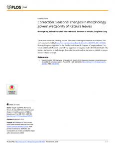
representing a grassland and a pine plantation (Fig. 1), expressing the most different
239
phenology in the study area, to extract seasonal amplitude, noise level, and average value.
240
Simulated NDVI time series are generated by summing individually simulated seasonal,
241
noise, and trend components. First, the seasonal component is created using an asymmetric
8
242
Gaussian function for each season. This Gaussian-type function has been shown to perform
243
well when used to extract seasonality by fitting the function to time series (J¨onsson and
244
Eklundh, 2002). The amplitude of the MODIS NDVI time series was estimated using the
245
range of the seasonal component derived with the STL function, as shown in Fig. 2. The
246
estimated seasonal amplitudes of the real forest and grassland MODIS NDVI time series
247
were 0.1 and 0.5 (Fig. 1). Second, the noise component was generated using a random
248
number generator that follows a normal distribution N(𝜇 = 0, 𝜎 = 𝑥), where the estimated
249
𝑥 values were 0.04 and 0.02, to approximate the noise within the real grass and forest
250
MODIS NDVI time series (Lhermitte et al., submitted). Vegetation index specific noise was
251
generated by randomly replacing the white noise by noise with a value of −0.1, representing
252
cloud contamination that often remains after atmospheric correction and cloud masking
253
procedures. Third, the real grass and forest MODIS NDVI time series were approximated
254
by selecting constant values 0.6 and 0.8 and summing them with the simulated noise and
255
seasonal component. A comparison between real and simulated NDVI time series is shown
256
in Fig. 1.
257
Based on the parameters required to simulate NDVI time series similar to the real grass
258
and forest MODIS NDVI time series (Fig. 1), we selected a range of amplitude and noise
259
values for the simulation study (Table 1). These values are used to simulate NDVI time
260
series of different quality (i.e. varying signal to noise ratios) representing a large range of
261
land cover types. Table 1: Parameter values for simulation of 16-day NDVI time series Parameters Amplitude 𝜎 Noise Magnitude
Values 0.1, 0.3, 0.5 0.01, 0.02, . . . , 0.07 −0.3, −0.2, −0.1, 0
262
The accuracy of the method for estimating the number, timing and magnitude of abrupt
263
changes was assessed by adding disturbances with a specific magnitude to the simulated
264
time series. A simple disturbance was simulated by combining a step function with a
265
specific magnitude (Table 1) and linear recovery phase (Kennedy et al., 2007). As such,
266
the disturbance can be used to simulate, for example, a fire in a grassland or an insect
267
attack on a forest. Three disturbances were added to the simulated seasonal, trend, and
268
noise components using simulation parameters (Table 1). An example of a simulated NDVI 9
269
time series with three disturbances is shown in Fig. 3. A Root Mean Square Error (RMSE)
270
was derived for 500 iterations of all the combinations of amplitude, noise and magnitude of
271
change levels to quantify the accuracy of estimating: (1) the number of detected changes,
272
(2) the time of change, and (3) the magnitude of change.
273
3.2. Spatial application on MODIS image time series
274
We apply BFAST to real remotely sensed time series, and compare the detected changes
275
with a spatial validation data set. BFAST provides information on the number, time,
276
magnitude and direction of changes in the trend and seasonal components of a time series.
277
We focussed on the timing and magnitude of major changes occurring within the trend
278
component.
279
We selected the 16-day MODIS NDVI composites with a 250m spatial resolution
280
(MOD13Q1 collection 5), since this product provides frequent information at the spatial
281
scale at which the majority of human-driven land cover changes occur (Townshend and
282
Justice, 1988). The MOD13Q1 16-day composites were generated using a constrained view
283
angle maximum NDVI value compositing technique (Huete et al., 2002). The MOD13Q1
284
images were acquired from the February 24th of 2000 to the end of 2008 (23 images/year
285
except for the year 2000) for a multi-purpose forested study area (Pinus radiata plantation)
286
in South Eastern Australia (Lat. 35.5∘ S, Lon. 148.0∘ E). The images contain data from
287
the red (620–670nm) and near-infrared (NIR, 841–876nm) spectral wavelengths. We used
288
the binary MODIS Quality Assurance flags to select only cloud-free data of optimal quality.
289
The quality flags, however, do not guarantee cloud-free data for the MODIS 250 m pixels
290
since that algorithms used to screen clouds use bands at coarse resolution. Missing values
291
are replaced by linear interpolation between neighboring values within the NDVI series
292
(Verbesselt et al., 2006).
293
The 16-day MODIS NDVI image series were analyzed, and the changes revealed were
294
compared with spatial forest inventory information on the ’year of planting’ of Pinus
295
radiata. Time of change at a 16-day resolution was summarized to a yearly temporal
296
resolution to facilitate comparison with the validation data. The validation protocol was
297
applied under the assumption that no other major disturbances (e.g. tree mortality) would
298
occur that would cause a change in the NDVI time series bigger than the change caused
299
by harvesting and planting activities.
10
300
4. Results
301
4.1. Simulated NDVI time series
302
Fig. 3 illustrates how BFAST decomposes and fits different time series components. It
303
can be seen that the fitted and simulated components are similar, and that the magnitude
304
and timing of changes in the trend component are correctly estimated. The accuracies
305
(RMSE) of the number of estimated changes are summarized in Fig. 4. Only results for
306
seasonal amplitude 0.1 and 0.5 are shown but similar results were obtained for 0.3 NDVI
307
amplitude. Three properties of the method are illustrated. First, the noise level only has
308
an influence on the estimation of the number of changes when the magnitude of the change
309
is -0.1, and is smaller than the overall noise level. The noise level is expressed as 4 𝜎, i.e.
310
99% of the noise range, to enable a comparison with the magnitude (Fig. 4). Second, the
311
noise level does not influence the RMSE when no changes are simulated (magnitude =
312
0), indicating a low commission error independent of the noise level. Third, the seasonal
313
amplitude does not have an influence on the accuracy of change detection. In Fig. 5 only
314
simulation results for an amplitude 0.1 are shown, since similar results were obtained for
315
other amplitudes (0.3 and 0.5). Overall, Fig. 5 illustrates that the RMSE of estimating the
316
time and magnitude of change estimation is small and increases slowly for increasing noise
317
levels. Only when the magnitude of change is small (−0.1) compared to the noise level
318
(> 0.15), the RMSE increases rapidly for increasing noise levels.
319
4.2. Spatial application on MODIS image time series
320
The application of BFAST to MODIS NDVI time series of a Pinus radiata plantation
321
produced estimates of the time and magnitude of major changes. These results are shown
322
spatially in Figs. 6 and 7. The time of change estimated by BFAST is summarized
323
each year to facilitate comparison. Only areas for which we had validation data available
324
were visualized in Figs. 6 and 7. The overall similarity between the time of planting
325
and time of detected change illustrates how BFAST can be used to detect change in a
326
forest plantation (Fig. 6). However, differences in the estimated time of change can be
327
interpreted using differences in the magnitude of change estimated by BFAST. Fig. 7
328
shows that detected changes can have either a positive or a negative magnitude of change.
329
This can be explained by the fact that planting in pine plantations in the study area
330
corresponds with a harvesting operation in the preceding year (personal communication 11
331
with C. Stone). Harvesting operations cause a significant decrease in the NDVI times series,
332
whereas planting causes a more gradual increase in NDVI. Firstly, if planting occurred
333
before 2002, the NDVI time series did not contain any significant decrease in NDVI caused
334
by the harvesting operations, since the MODIS NDVI time series only started in early
335
2000. BFAST therefore detected change with a positive magnitude, indicating regrowth
336
(Fig. 7), corresponding to a time of change during or later than the plant date (Fig. 6).
337
Fig. 8 (top) illustrates detected changes within a NDVI time series extracted from a single
338
MODIS pixel within a pine plantation with a planting activity during 2001. Secondly,
339
if planting occurred after 2003, the time series contained a significant decrease in NDVI
340
caused by the harvesting operations. Major change detected as a consequence are changes
341
corresponding to harvesting preceding the planting operation, and are therefore detected
342
before the planting date (Fig. 6) and have a negative magnitude (Fig. 7). Fig. 8 (middle)
343
illustrates detected changes within a NDVI time series with harvesting operation activity
344
during 2004. These points illustrate BFAST’s capacity to detect and characterize change,
345
but also confirm the importance of simulating time series in a controlled environment, since
346
it is very difficult to find validation data to account for all types of change occurring in
347
ecosystems.
348
Fig. 8 (bottom) shows an example of changes detected by BFAST in an area where
349
harvesting and thinning activities were absent. Fig. 9 illustrates how BFAST decomposed
350
the NDVI time series and fitted seasonal, trend and remainder components. In 2002 and
351
2006 the study area experienced a severe drought, which caused the pine plantations to
352
be stressed and the NDVI to decrease significantly. Severe tree mortality occurred in
353
2006, since trees were drought-stressed and not able to defend themselves against insect
354
attacks (Verbesselt et al., in press). This explains why the change detected in 2006 is
355
bigger (magnitude of the abrupt change) and the recovery (slope of the gradual change) is
356
slower than the change detected in 2003, as shown in (Fig. 9). This example illustrates
357
how the method could be used to detect and characterize changes related to forest health.
358
5. Discussion and further work
359
The main characteristics of BFAST are revealed by testing the approach using simulated
360
time series and by comparing detected changes in 16-day MODIS NDVI time series with
361
spatial forest inventory data. Simulation of NDVI time series illustrated that the iterative 12
362
decomposition of time series into a seasonal and trend component was not influenced by
363
the seasonal amplitude and by noise levels smaller than the simulated change magnitude.
364
This enabled the robust detection of abrupt and gradual changes in the trend component.
365
As such, full time series can be analyzed without having to select only data during a
366
specific period (e.g. growing season), or can avoid the normalization of reflectance values
367
for each land cover type to minimize seasonal variability (Healey et al., 2005; Hilker et al.,
368
2009). Seasonal adjustment by decomposing time series, as implemented in the BFAST
369
approach, facilitates the detection of change in the trend component independent of seasonal
370
amplitude or land cover type information. Considerations for further research fall into
371
three main categories:
372
(1) Further research is necessary to study BFAST’s sensitivity to detecting phenological
373
change in the seasonal component. This research has focussed on the detection and
374
characterization of changes within the trend component of 16-day NDVI time series.
375
Changes in the seasonal component were not simulated, and BFAST’s sensitivity to
376
detecting seasonal changes using simulated data was not assessed. However, changes
377
occurring in the seasonal component can be detected using BFAST. The application of
378
BFAST to 16-day MODIS NDVI time series on a forested area (40000ha) revealed that
379
seasonal breaks were detected in only 5% of the area. The small number of seasonal
380
breaks occurring in the study area could be explained by the fact that a seasonal
381
change is only detected when a change between land cover types with a significantly
382
different phenology occurs. Time series with a higher temporal resolution (e.g. daily or
383
8-day) could increase the accuracy of detecting seasonal changes but might also impact
384
the ability to detect subtle changes due to higher noise levels. Zhang et al. (2009)
385
illustrated that vegetation phenology can be estimated with high accuracy (absolute
386
error of less than 3 days) in time series with a temporal resolution of 6–16 days, but
387
that accuracy depends on the occurrence of missing values. It is therefore necessary to
388
study BFAST’s capacity to detect phenological change caused by climate variations or
389
land use change in relation to the temporal resolution of remotely sensed time series.
390
(2) Future algorithm improvements may include the capacity to add functionality to
391
identify the type of change with information on the parameters of the fitted piecewise
392
linear models (e.g. intercept and slope). In this study we have focussed on the
393
magnitude of change, derived using Eq. 2, but the spatial application on MODIS NDVI 13
394
time series illustrated that change needs to be interpreted by combining the time and
395
magnitude of change. Alternatively, different change types can be identified based
396
on whether seasonal and trend breaks occur at the same time or not and whether a
397
discontinuity occurs (i.e. magnitude > 0) (Shao and Campbell, 2002). Parameters of
398
the fitted piecewise linear models can also be used to compare long term vegetation
399
trends provided by different satellite sensors. Fensholt et al. (2009), for example,
400
used linear models to analyze trends in annually integrated NDVI time series derived
401
from Advanced Very High Resolution Radiometer (AVHRR), SPOT VEGETATION,
402
and MODIS data. BFAST enables the analysis of long NDVI time series and avoids
403
the need to summarize data annually (i.e. loss of information) by accounting for the
404
seasonal and trend variation within time series. This illustrates that further work is
405
needed to extend the method from detecting change to classifying the type of change
406
detected.
407
(3) Evaluating BFAST’s behavior for different change types (e.g. fires versus desertification)
408
in a wide variety of ecosystems remains important. BFAST is tested by combining
409
different magnitudes of an abrupt change with a large range of simulated noise and
410
seasonal variations representing a large range of land cover types. BFAST is able to
411
detect different change types, however, it remains important to understand how these
412
change types (e.g. woody encroachment) will be detected in ecosystems with drastic
413
seasonal changes (e.g. strong and variable tropical dry seasons) and severe noise in the
414
spectral signal (e.g. sun angle and cloud cover in mountainous regions).
415
(4) The primary challenge of MODIS data, despite its high temporal resolution, is to
416
extract useful information on land cover changes when the processes of interest operate
417
at a scale below the spatial resolution of the sensor (Hayes and Cohen, 2007). Landsat
418
data have been successfully applied to detect changes at a 30m spatial resolution.
419
However, the temporal resolution of Landsat, i.e. 16-day, which is often extended by
420
cloud cover, can be a major obstacle. The fusion of MODIS with Landsat images to
421
combine high spatial and temporal resolutions has helped to improve the mapping of
422
disturbances (Hilker et al., 2009). It is our intention to use BFAST in this integrated
423
manner to analyze time series of multi-sensor satellite images, and to be integrated
424
with data fusion techniques.
14
425
This research fits within an Australian forest health monitoring framework, where
426
MODIS data is used as a ‘first pass’ filter to identify the regions and timing of major
427
change activity (Stone et al., 2008). These regions would be targeted for more detailed
428
investigation using ground and aerial surveys, and finer spatial and spectral resolution
429
imagery.
430
6. Conclusion
431
We have presented an generic approach for detection and characterization of change in
432
time series. ‘Breaks For Additive Seasonal and Trend’ (BFAST) enables the detection of
433
different types of changes occurring in time series. BFAST integrates the decomposition of
434
time series into trend, seasonal, and remainder components with methods for detecting
435
multiple changes. BFAST iteratively estimates the dates and number of changes occur-
436
ring within seasonal and trend components, and characterizes changes by extracting the
437
magnitude and direction of change. Changes occurring in the trend component indicate
438
gradual and abrupt change, while changes occurring in the seasonal component indicate
439
phenological changes. The approach can be applied to other time series data without the
440
need to select specific land cover types, select a reference period, set a threshold, or define
441
a change trajectory.
442
Simulating time series with varying amounts of seasonality and noise, and by adding
443
abrupt changes at different times and magnitudes, revealed that BFAST is robust against
444
noise, and is not influenced by changes in amplitude of the seasonal component. This
445
confirmed that BFAST can be applied to a large range of time series with varying noise
446
levels and seasonal amplitudes, representing a wide variety of ecosystems. BFAST was
447
applied to 16-day MODIS NDVI image time series (2000–2008) for a forested study area
448
in south eastern Australia. This showed that BFAST is able to detect and characterize
449
changes by estimating time and magnitude of changes occurring in a forested landscape.
450
The algorithm can be extended to label changes with their estimated magnitude and
451
direction. BFAST can be used to analyze different types of remotely sensed time series
452
(AVHRR, MODIS, Landsat) and can be applied to other disciplines dealing with seasonal
453
or non-seasonal time series, such as hydrology, climatology, and econometrics. The R code
454
(R Development Core Team, 2008) developed in this paper is available by contacting the
455
authors. 15
456
457
7. Acknowledgements This work was undertaken within the Cooperative Research Center for Forestry Pro-
458
gram 1.1: Monitoring and Measuring (www.crcforestry.com.au). Thanks to Dr. Achim
459
Zeileis for support with the ‘strucchange’ package in R, to professor Nicholas Coops, Dr.
460
Geoff Laslett, and the four anonymous reviewers whose comments greatly improved this
461
paper.
462
References
463
Anyamba, A., Eastman, J. R., 1996. Interannual variability of NDVI over Africa and
464
its relation to El Nino Southern Oscillation. International Journal of Remote Sensing
465
17 (13), 2533–2548.
466
Azzali, S., Menenti, M., 2000. Mapping vegetation-soil-climate complexes in southern
467
Africa using temporal Fourier analysis of NOAA-AVHRR NDVI data. International
468
Journal of Remote Sensing 21 (5), 973–996.
469
470
Bai, J., Perron, P., 2003. Computation and analysis of multiple structural change models. Journal of Applied Econometrics 18 (1), 1–22.
471
Bontemps, S., Bogaert, P., Titeux, N., Defourny, P., 2008. An object-based change detection
472
method accounting for temporal dependences in time series with medium to coarse spatial
473
resolution. Remote Sensing of Environment 112 (6), 3181–3191.
474
Cleveland, R. B., Cleveland, W. S., McRae, J. E., Terpenning, I., 1990. STL: A seasonal-
475
trend decomposition procedure based on loess. Journal of Official Statistics 6, 3–73.
476
Coppin, P., Jonckheere, I., Nackaerts, K., Muys, B., Lambin, E., 2004. Digital change
477
detection methods in ecosystem monitoring: a review. International Journal of Remote
478
Sensing 25 (9), 1565–1596.
479
Crist, E. P., Cicone, R. C., 1984. A physically-based transformation of thematic mapper
480
data – The TM tasseled cap. IEEE Transactions on Geoscience and Remote Sensing
481
22 (3), 256–263.
482
483
de Beurs, K. M., Henebry, G. M., 2005. A statistical framework for the analysis of long image time series. International Journal of Remote Sensing 26 (8), 1551–1573. 16
484
DeFries, R. S., Field, C. B., Fung, I., Collatz, G. J., Bounoua, L., 1999. Combining satellite
485
data and biogeochemical models to estimate global effects of human-induced land cover
486
change on carbon emissions and primary productivity. Global Biogeochemical Cycles
487
13 (3), 803–815.
488
Dixon, R. K., Solomon, A. M., Brown, S., Houghton, R. A., Trexier, M. C., Wisniewski, J.,
489
1994. Carbon pools and flux of global forest ecosystems. Science 263 (5144), 185–190.
490
Fensholt, R., Rasmussen, K., Nielsen, T. T., Mbow, C., 2009. Evaluation of earth ob-
491
servation based long term vegetation trends – intercomparing NDVI time series trend
492
analysis consistency of Sahel from AVHRR GIMMS, Terra MODIS and SPOT VGT
493
data. Remote Sensing of Environment 113 (9), 1886 – 1898.
494
Hayes, D. J., Cohen, W. B., 2007. Spatial, spectral and temporal patterns of tropical forest
495
cover change as observed with multiple scales of optical satellite data. Remote Sensing
496
of Environment 106 (1), 1–16.
497
Haywood, J., Randal, J., 2008. Trending seasonal data with multiple structural breaks.
498
NZ visitor arrivals and the minimal effects of 9/11. Research report 08/10, Victoria
499
University of Wellington, New Zealand.
500
URL
501
mscs08-10.pdf
http://msor.victoria.ac.nz/twiki/pub/Main/ResearchReportSeries/
502
Healey, S. P., Cohen, W. B., Zhiqiang, Y., Krankina, O. N., 2005. Comparison of Tasseled
503
Cap-based Landsat data structures for use in forest disturbance detection. Remote
504
Sensing of Environment 97 (3), 301–310.
505
Hilker, T., Wulder, M. A., Coops, N. C., Linke, J., McDermid, G., Masek, J. G., Gao, F.,
506
White, J. C., 2009. A new data fusion model for high spatial- and temporal-resolution
507
mapping of forest disturbance based on Landsat and MODIS. Remote Sensing of Envi-
508
ronment 113 (8), 1613–1627.
509
Huete, A., Didan, K., Miura, T., Rodriguez, E. P., Gao, X., Ferreira, L. G., 2002. Overview
510
of the radiometric and biophysical performance of the MODIS vegetation indices. Remote
511
Sensing of Environment 83 (1-2), 195–213.
17
512
513
Jin, S. M., Sader, S. A., 2005. MODIS time-series imagery for forest disturbance detection and quantification of patch size effects. Remote Sensing of Environment 99 (4), 462–470.
514
J¨onsson, P., Eklundh, L., 2002. Seasonality extraction by function fitting to time-series
515
of satellite sensor data. IEEE Transactions on Geoscience and Remote Sensing 40 (8),
516
1824–1832.
517
Kennedy, R. E., Cohen, W. B., Schroeder, T. A., 2007. Trajectory-based change detection
518
for automated characterization of forest disturbance dynamics. Remote Sensing of
519
Environment 110 (3), 370–386.
520
Lambin, E. F., Strahler, A. H., 1994. Change-Vector Analysis in multitemporal space - a
521
tool to detect and categorize land-cover change processes using high temporal-resolution
522
satellite data. Remote Sensing of Environment 48 (2), 231–244.
523
Lhermitte, S., Verbesselt, J., Verstraeten, W. W., Coppin, P., submitted. Comparison of
524
time series similarity measures for monitoring ecosystem dynamics: a review of methods
525
for time series clustering and change detection. Remote Sensing of Environment.
526
527
528
529
Lu, D., Mausel, P., Brondizio, E., Moran, E., 2004. Change detection techniques. International Journal of Remote Sensing 25 (12), 2365–2407. Makridakis, S., Wheelwright, S. C., Hyndman, R. J., 1998. Forecasting: methods and applications, 3rd Edition. John Wiley & Sons, New York.
530
Myneni, R. B., Hall, F. G., Sellers, P. J., Marshak, A. L., 1995. The interpretation of
531
spectral vegetation indexes. IEEE Transactions on Geoscience and Remote Sensing
532
33 (2), 481–486.
533
R Development Core Team, 2008. R: A Language and Environment for Statistical Com-
534
puting. R Foundation for Statistical Computing, Vienna, Austria.
535
URL www.R-project.org
536
Roy, D. P., Borak, J. S., Devadiga, S., Wolfe, R. E., Zheng, M., Descloitres, J., 2002. The
537
MODIS Land product quality assessment approach. Remote Sensing of Environment
538
83 (1-2), 62–76.
18
539
Shao, Q., Campbell, N. A., 2002. Modelling trends in groundwater levels by segmented
540
regression with constraints. Australian & New Zealand Journal of Statistics 44 (2),
541
129–141.
542
Stone, C., Turner, R., Verbesselt, J., 2008. Integrating plantation health surveillance
543
and wood resource inventory systems using remote sensing. Australian Forestry 71 (3),
544
245–253.
545
Townshend, J. R. G., Justice, C. O., 1988. Selecting the spatial-resolution of satellite
546
sensors required for global monitoring of land transformations. International Journal of
547
Remote Sensing 9 (2), 187–236.
548
549
550
551
552
Tucker, C. J., 1979. Red and photographic infrared linear combinations for monitoring vegetation. Remote Sensing of Environment 8 (2), 127–150. Venables, W. N., Ripley, B. D., 2002. Modern applied statistics with S, 4th Edition. Springer-Verlag, pp. 156–163. Verbesselt, J., J¨onsson, P., Lhermitte, S., van Aardt, J., Coppin, P., 2006. Evaluating
553
satellite and climate data derived indices as fire risk indicators in savanna ecosystems.
554
IEEE Transactions on Geoscience and Remote Sensing 44 (6), 1622–1632.
555
Verbesselt, J., Robinson, A., Stone, C., Culvenor, D., in press. Forecasting tree mortality
556
using change metrics derived from MODIS satellite data. Forest Ecology and Management,
557
doi:10.1016/j.foreco.2009.06.011.
558
559
560
561
562
563
Zeileis, A., 2005. A unified approach to structural change tests based on ML scores, F statistics, and OLS residuals. Econometric Reviews 24 (4), 445 – 466. Zeileis, A., Kleiber, C., 2005. Validating multiple structural change models – A case study. Journal of Applied Econometrics 20 (5), 685–690. Zeileis, A., Kleiber, C., Kr¨amer, W., Hornik, K., 2003. Testing and dating of structural changes in practice. Computational Statistics and Data Analysis 44, 109–123.
564
Zeileis, A., Leisch, F., Hornik, K., Kleiber, C., 2002. strucchange: An R package for testing
565
for structural change in linear regression models. Journal of Statistical Software 7 (2),
566
1–38. 19
567
Zhang, X., Friedl, M., Schaaf, C., 2009. Sensitivity of vegetation phenology detection to
568
the temporal resolution of satellite data. International Journal of Remote Sensing 30 (8),
569
2061–2074.
20
0.90
0.3
0.5
0.7
0.9
to the web version of this article.
0.80
Real Simulated
0.70
572
For interpretation of the references to color in this figure legend, the reader is referred
NDVI
571
Figures
NDVI
570
2000
2002
2004
2006
2008
Time
Figure 1: Real and simulated 16-day NDVI time series of a grassland (top) and pine plantation (bottom).
21
0.90 0.80 0.70
data
0.78
0.82
−0.04
0.02
seasonal trend
−0.05
0.05
remainder 2000
2002
2004
2006
2008
time
Figure 2: The STL decomposition of a 16-day NDVI time series of a pine plantation into seasonal, trend, and remainder components. The seasonal component is estimated by taking the mean of all seasonal sub-series (e.g. for a monthly time series the first sub-series contains the January values). The sum of the seasonal, trend, and remainder components equals the data series. The solid bars on the right hand side of the plot show the same data range, to aid comparisons. The range of the seasonal amplitude is approximately 0.1 NDVI.
22
0.9 0.6
0.20
0.3
data
−0.10
0.00
0.40
0.55
0.70
−0.10
0.05
seasonal trend remainder
2000
2002
2004
2006
2008
Time
Figure 3: Simulated 16-day MODIS NDVI time series with a seasonal amplitude = 0.3, 𝜎 = 0.02 and change magnitude = -0.3. The simulated data series is the sum of the simulated seasonal, trend and noise series (- - -), and is used as an input in BFAST. The estimated seasonal, trend and remainder series are shown in red. Three break points are detected within the estimated trend component (⋅ ⋅ ⋅ ). The solid bars on the right hand side of the plot show the same data range, to aid comparisons.
23
m = −0.1
m = −0.2
m = −0.3
a = 0.1
m=0 a = 0.5
2.0
RMSE
1.5
1.0
0.5
0.0 0.05
0.10
0.15
0.20
0.25
0.05
0.10
0.15
0.20
0.25
Noise
Figure 4: RMSEs for the estimation of number of abrupt changes within a time series, as shown in Figure 3 (a = amplitude of the seasonal component, m = magnitude of change). The units of the 𝑥 and 𝑦-axes are 4𝜎 (noise) and the number of changes (RMSE). See Table 1 for the values of parameters used for the simulation of the NDVI time series. Similar results were obtained for a = 0.3
24
m = −0.1
m = −0.2
m = −0.3
m=0 Magnitude a = 0.1
0.06 0.04
6 0
2
0.02
4
RMSE
8
10
0.08
Time a = 0.1
0.05
0.10
0.15
0.20
0.25
0.05
0.10
0.15
0.20
0.25
Noise
Figure 5: RMSEs for the estimation of the time and magnitude of abrupt changes within a time series (a = amplitude of the seasonal component, m = magnitude of changes). The units of the 𝑥-axis are 4𝜎 NDVI, and 𝑦-axis are relative time steps between images (e.g. 1 equals a 16-day period) (left) and NDVI (right). See Table 1 for the values of parameters used for the simulation of NDVI time series. Similar results were obtained for a = 0.3 and 0.5.
25
148 4’0"E
148 6’0"E
148 8’0"E
Year of planting 2001 2002 2003 2004 2005 2006
Year of change 2001 2002 2003 2004 2005 2006
0
1
2
4
6
Kilometers
148 0’0"E
148 2’0"E
148 4’0"E
148 6’0"E
35 35’0"S 35 34’0"S 35 33’0"S 35 32’0"S 35 31’0"S 35 30’0"S 35 29’0"S 35 28’0"S 35 27’0"S 35 26’0"S 35 25’0"S
148 2’0"E
35 35’0"S 35 34’0"S 35 33’0"S 35 32’0"S 35 31’0"S 35 30’0"S 35 29’0"S 35 28’0"S 35 27’0"S 35 26’0"S 35 25’0"S
148 0’0"E
148 8’0"E
Figure 6: Comparison between the year of Pinus radiata planting derived from spatial forest inventory data and the BFAST estimate of the year of major change occurring in MODIS NDVI image time series (2000–2008) for a forested area in south eastern Australia.
26
148 4’0"E
148 6’0"E
148 8’0"E
NDVI -0.48 - -0.37 -0.36 - -0.29 -0.28 - -0.2 -0.19 - -0.1 -0.09 - 0 0.01 - 0.12 0.13 - 0.23
0
1
2
4
6
Kilometers
148 0’0"E
148 2’0"E
148 4’0"E
148 6’0"E
35 35’0"S 35 34’0"S 35 33’0"S 35 32’0"S 35 31’0"S 35 30’0"S 35 29’0"S 35 28’0"S 35 27’0"S 35 26’0"S 35 25’0"S
148 2’0"E
35 35’0"S 35 34’0"S 35 33’0"S 35 32’0"S 35 31’0"S 35 30’0"S 35 29’0"S 35 28’0"S 35 27’0"S 35 26’0"S 35 25’0"S
148 0’0"E
148 8’0"E
Figure 7: BFAST estimated magnitudes of major changes occurring in MODIS NDVI image time series (2000–2008) for a forested area in south eastern Australia. Negative values generally indicate harvesting, while positive values indicate forest growth.
27
0.9 0.7 NDVI
0.5
0.7
0.9
0.3
0.3
0.5
NDVI 0.90 0.80
NDVI
0.70 2000
2002
2004
2006
2008
Figure 8: Detected changes in the trend component (red) of 16-day NDVI time series (black) extracted from a single MODIS pixel within a pine plantation, that was planted in 2001 (top), harvested in 2004 (middle), and with tree mortality occurring in 2007 (bottom). The time of change (- - -), together with its confidence intervals (red) are also shown.
28
0.90 0.80
0.04
0.70
data
0.76
0.82
−0.04
0.00
seasonal trend
−0.05
0.05
remainder 2000
2002
2004
2006
2008
Time
Figure 9: Fitted seasonal, trend and remainder (i.e. estimated noise) components for a 16-day MODIS NDVI time series (data series) of a pine plantation in the northern part of the study area. Three abrupt changes are detected in the trend component of the time series. Time (- - -), corresponding confidence interval (red), direction and magnitude of abrupt change and slope of the gradual change are shown in the estimated trend component. The solid bars on the right hand side of the plot show the same data range, to aid comparisons.
29