Hindawi Publishing Corporation Journal of Sensors Volume 2013, Article ID 393406, 12 pages http://dx.doi.org/10.1155/2013/393406
Research Article Development of an Optical Sensor Head for Current and Temperature Measurements in Power Systems Fábio V. B. de Nazaré, Marcelo M. Werneck, Rodrigo P. de Oliveira, D. M. Santos, R. C. Allil, and B. A. Ribeiro Laborat´orio de Instrumentac¸a˜ o e Fotˆonica, Universidade Federal do Rio de Janeiro, Avenida Hor´acio Macedo 2030, Ilha do Fund˜ao, Centro de Tecnologia, Bloco I—036 (subsolo), Rio de Janeiro, 21941-914 RJ, Brazil Correspondence should be addressed to F´abio V. B. de Nazar´e;
[email protected] Received 13 December 2012; Revised 22 February 2013; Accepted 21 March 2013 Academic Editor: Rong Zeng Copyright © 2013 F´abio V. B. de Nazar´e et al. This is an open access article distributed under the Creative Commons Attribution License, which permits unrestricted use, distribution, and reproduction in any medium, provided the original work is properly cited. The development of a current and temperature monitoring optical device intended to be used in high-voltage environments, particularly transmission lines, is presented. The system is intended to offer not only measurement reliability, but to be also practical and light weighted. Fiber Bragg gratings (FBGs) are employed in the measurement of both physical parameters: the current will be acquired using a hybrid sensor head setup—an FBG fixed on a magnetostrictive rod—while a single-point temperature information is provided by a dedicated grating. An inexpensive and outdoor-suitable demodulation method, such as the fixed filter technique, should be used in order to improve the instrumentation robustness, avoiding expensive and complex auxiliary electronics. The preliminary results for laboratory tests are also discussed.
1. Introduction Unfailing measurements in power systems are obligatory in various situations, such as in substations, in oil industry, and in power transmission [1, 2]. Particularly, parameters of transmission lines such as temperature and conductor current should be monitored, providing important data for ampacity assessment [2]. Though, usual instrument transformers in electric power facilities present significant size, besides being heavy. Numerous optical current sensing devices that make use of the Faraday effect have been discussed, since optical systems frequently offer a wider dynamic range, lighter weight, improved safety, and electromagnetic interference immunity [3], due to the intrinsic insulating aspects of optical fibers. Nevertheless, some drawbacks can be mentioned; the Faraday Effect, besides requiring complex compensation techniques, also demands expensive auxiliary electronics, maintenance, and specially designed optical fibers to become reliable. So far, optical fiber sensors (OFSs) have been highly employed in environments where the use of electrical sensors is not reliable or may create unsafe circumstances. What
makes this possible is the use of fiber Bragg gratings— intrinsic optical fiber sensors which are, frequently, wavelength demodulated, requiring the use of a piece of equipment called optical spectrum analyzer (OSA) [4]. Despite its reliability, the wavelength demodulation procedure implies the use of high-cost equipments to attend the high spectral resolution monitoring requirements, a rather restrictive aspect for outdoor monitoring. Quite a few designs of hybrid optical current sensors have been presented; some of which explore the magnetostrictive actuation of a ferromagnetic rod over a fiber Bragg grating, which is attached to this material [5, 6]. Still, commonly proposed demodulation techniques are expensive or not suitable for a prolonged operation in harsh environments. The first development stages of an optical current transducer are discussed in the first part of this paper. A laboratory test device for Terfenol-D, an alloy that presents a positive magnetostriction, is shown, and the designed magnetooptical sensor head is tested. Subsequently, the temperature measurement section of the system is presented. An FBG is employed as a fixed spectral filter; this filter works as a spectral response interrogator
2
Journal of Sensors
of a sensing FBG, which is submitted to an induced and controlled temperature variation. Simulations are carried out during this study, and after that a single-point measurement system is investigated. Such optical system has the potential to reduce the costs of an optical fiber sensing arrangement, enabling the measurement of dynamic parameters where high voltage levels are present.
2. Theory and Background 2.1. Optical Fiber Bragg Gratings Theory. Fiber Bragg gratings are simple and passive devices, which consist of modulations of the refractive index (RI) of the core of optical fibers. This technology is one of the most popular choices for optical fiber sensors for strain or temperature measurements due to their simple manufacturing and due to the relatively strong reflected signal. The term fiber Bragg grating was borrowed from the Bragg law and applied to the periodical structures inscribed inside the core of conventional telecom fiber. Bragg diffraction occurs for an electromagnetic radiation when wavelength is of the same order of magnitude of the atomic spacing, if incident upon a crystalline material. In this case, the radiation is scattered in a specular fashion by the atoms of the material and experiences a constructive interference in accordance to Bragg’s law. For a crystalline solid with lattice planes separated by a distance 𝑑, the waves are scattered and interfere constructively if the path length of each wave is equal to an integer multiple of the wavelength. Figure 1 shows this idea, and Bragg’s law describes the condition for constructive interference from several crystallographic planes of the crystalline lattice separated by a distance 𝑑: 2𝑑 sin 𝜃 = 𝑛𝜆,
(1)
where 𝜃 is the incident angle, 𝑛 is an integer, and 𝜆 is the wavelength. A diffraction pattern is obtained by measuring the intensity of the scattered radiation as a function of 𝜃. Whenever the scattered waves satisfy the Bragg condition, a strong intensity in the diffraction pattern is observed, known as Bragg’s peak. So, after the inscription of the grating into the optical fiber core, due to the periodic modulation of the index of refraction, light guided along the core of the fiber will be weakly reflected by each grating plane according to the Fresnel effect. The reflected light from each grating plane will join together with the other reflections in the backward direction. This addition may be constructive or destructive, depending on whether the wavelength of the incoming light meets the Bragg condition described by (1). Now, according to (1), since 𝜃 = 90∘ and d is the distance between peaks of the interference pattern, 𝜆 = 2𝑑 for 𝑛 = 1 is the approximate reflection peak wavelength. That is, the fiber now acts as a dichroic mirror, reflecting part of the incoming spectrum. Equation (1), developed for vacuum, has to be adapted for silica, since the distances traveled by light are affected by the index of refraction of the fiber: 𝜆 𝐵 = 2𝑛eff Λ.
(2)
Therefore, the Bragg wavelength (𝜆 𝐵 ) of an FBG is a function of the effective refractive index of the fiber (𝑛eff ) and the periodicity of the grating (Λ). Essentially, any external agent that is capable of changing Λ will displace the reflected spectrum centered at Bragg’s wavelength. A longitudinal deformation, due to an external force, for instance, may change both Λ and 𝑛eff , the latter by the photoelastic effect and the former by increasing the pitch of the grating. Equally, a variation in temperature can also change both parameters, via thermal dilation and thermooptic effect, respectively. Therefore, an FBG is essentially a sensor of temperature and strain but, by designing the proper interface, many other measurands can be made to impose perturbation on the grating resulting in a shift in the Bragg wavelength, which can then be used as a parameter transducer. Therefore, by using an FBG as a sensor one can obtain measurements of strain, temperature, pressure, vibration, displacement, and so forth. In order to calculate the sensitivity of the Bragg wavelength with temperature and strain, (2) must be used. Notice that the sensitivity with temperature is the partial derivative with respect of temperature 𝑇: 𝜕𝑛 Δ𝜆 𝐵 𝜕Λ = 2𝑛eff + 2Λ eff . Δ𝑇 𝜕𝑇 𝜕𝑇
(3)
Using (2) and (3), Δ𝜆 𝐵 1 𝜕Λ 1 𝜕𝑛eff = Δ𝑇 + Δ𝑇. 𝜆𝐵 Λ 𝜕𝑇 𝑛eff 𝜕𝑇
(4)
The first term is the thermal expansion of silica (𝛼) and the second term is the thermooptic coefficient (𝜂) representing the temperature dependence of the refractive index (𝑑𝑛/𝑑𝑇). Thus, Δ𝜆 𝐵 = (𝛼 + 𝜂) ⋅ Δ𝑇. 𝜆𝐵
(5)
The sensitivity with strain is the partial derivative of (2) with respect to displacement: 𝜕𝑛 Δ𝜆 𝐵 𝜕Λ = 2𝑛eff + 2Λ eff . Δ𝐿 𝜕𝐿 𝜕𝐿
(6)
Substituting twice (2) in (5), Δ𝜆 𝐵 1 𝜕Λ 1 𝜕𝑛eff = Δ𝐿 + Δ𝐿. 𝜆𝐵 Λ 𝜕𝐿 𝑛eff 𝜕𝐿
(7)
The first term in (7) is the strain of the grating period due to the extension of the fiber. If a stress of Δ𝐿 is applied, then a relative strain of Δ𝐿/𝐿 the FBG is obtained. At the same time if the FBG has a length 𝐿 FBG it will experience a strain Δ𝐿 FBG /𝐿 FBG , but since the FBG is inscribed in the fiber, then Δ𝐿 FBG /𝐿 FBG = Δ𝐿/𝐿. The Bragg displacement with extension equals the displacement of the grating period with the same extension; therefore, the first term in (7) is the unit. The second term in (7) is the photoelastic coefficient (𝜌𝑒 ), the variation of the index of refraction with strain.
Journal of Sensors
3
In some solids, depending on the Poisson ratio of the material, this effect is negative; that is, when a transparent medium expands, as an optical fiber for instance, the index of refraction decreases due to the decrease of density of the material. Then, when an extension is applied to the fiber, the two terms in (7) produce opposite effects, one by increasing the distance between gratings and thus augmenting the Bragg wavelength and the other by decreasing the effective RI and thus decreasing the Bragg wavelength. The combined effect of both phenomena is the classical form of the Bragg wavelength displacement with strain: Δ𝜆 𝐵 = (1 − 𝜌𝑒 ) 𝜀FBG , 𝜆𝐵
𝑑
(8)
Δ𝜆 𝐵 = 1.2 pm/𝜇𝜀. Δ𝜀
Terfenol-D rod 1000
Strain (𝜇𝜀)
800
(9)
where Δ𝜆 𝐵 is the Bragg wavelength shift, 𝜌𝑒 is the photoelastic coefficient (𝜌𝑒 = 0.22), 𝜀FBG is the strain, Δ𝑇 is the temperature variation, 𝛼 is the silica thermal expansion coefficient −1 (0.55 × 10⁻⁶ ∘ C ), and 𝜂 is thermooptic coefficient (8.6 × −1 10−6 ∘ C for Ge-doped silica optical fibers). Thus, the theoretical grating sensitivities to temperature and strain, at the wavelength range of 1550 nm, after substituting the constants in (9) are Δ𝜆 𝐵 = 14.18 pm/ ∘ C, Δ𝑇
𝑑sin 𝜃
Figure 1: An incident radiation is reflected by the lattice structure of a crystal and interferes constructively if the Bragg law is obeyed.
where 𝜀FBG is the longitudinal strain of the grating. Combining (5) and (8), the sensitivity of the Bragg wavelength with temperature and strain is obtained [8, 9]: Δ𝜆 𝐵 = (1 − 𝜌𝑒 ) 𝜀FBG + (𝛼 + 𝜂) ⋅ Δ𝑇, 𝜆𝐵
𝜃
600 400 200 0 −600
0 200 400 −400 −200 Magnetic field intensity (kA/m)
600
(a)
(10)
These theoretical values, presented in (10), though, are not absolute as each FBG will present slightly different sensitivities according to the manufacturing procedure, even for the same fabrication batch. 2.2. The Magnetostrictive Phenomenon. Magnetic materials present magnetostriction, a phenomenon in which the material suffers a strain due to the application of a magnetic field; that is, the magnetic sample shrinks (negative magnetostriction) or expands (positive magnetostriction) in the direction of magnetization [10]. Thus, magnetostrictive materials (MM) convert magnetic energy into mechanical energy, and the inverse is also true; that is, when the material suffers an external induced strain its magnetic state is changed. A typical length variation curve showed by a Terfenol-D rod when submitted to a magnetic field is presented in Figure 2(a), where in region A the saturation state has been reached. The strain characteristic showed in Figure 1 was obtained for a Terfenol-D rod, an alloy composed by iron, terbium, and dysprosium (a giant magnetostrictive material-GMM-) with dimensions of 80 mm × 10 mm × 10 mm, which is presented
10 mm
m
80 m
10 mm
(b)
Figure 2: (a) Terfenol-D strain characteristic; (b) Employed Terfenol-D rod.
in Figure 2(b). The material was submitted to a longitudinal magnetic field, generated by a laboratory electromagnet. As it can be seen in Figure 2(a), when the field direction is reversed, that is, the field is negative (e.g., when alternating magnetic fields are being employed), a strain with the same signal which would be obtained with a positive field is achieved. Thus, symmetric magnetic fields cause the same kind of strain (rectified response), and the resulting curve has a shape that is recalled a butterfly, and is in this way nicknamed.
4
Journal of Sensors Sensor FBG reflected spectrum
Optical fiber
Stretching device FBG
Optical intensity
Filter FBG reflected spectrum
FBG interrogator Magnetostrictive rod
Figure 4: FBG stretching scheme, prior to complete attachment.
Wavelength Intersection
Figure 3: Concept of the fixed filter demodulation method (adapted from [7]).
2.3. The Fixed Filter Demodulation Technique. Usually, two fiber Bragg gratings are used in simple measurement systems that employ the fixed filter technique. Beside the sensor FBG, a second grating called the filter FBG serves to interrogate the sensor FBG spectral response. When using this method, in addition to a pair of gratings, a broadband optical source and a photodetector are also needed for a practical implementation. Thus, the measurement information is obtained by exploring the reflected optical power, represented by the intersection region in Figure 3 [7]. This reflected power varies as the spectrum characteristic of the sensor FBG changes; as a result the fixed-filter approach requires a dedicated optoelectronic setup for each sensor [7].
3. Electrical Current Measurement Subsystem 3.1. FBG Attachment Procedure. The proposed current sensor subsystem is based on the sensitivity of the magnetostrictive material to the magnetic field—which is created by an electrical current in a conductor—and on the sensitivity of Bragg gratings to strain. Namely, when the dimensions of a MM are changed by a magnetic field this strain is transmitted to the attached FBG, enabling the measurement. On the other hand, Bragg gratings also present a sensitivity to the temperature variation, which influences the overall sensor operation. A fiber Bragg grating was fixed to the Terfenol-D rod using a commercial cyanoacrylate adhesive, after the cleaning of the surface. The FBG is also prior stretched, a procedure which will allow the monitoring of magnetoelastic elongations and compressions that the material suffers when submitted to AC magnetic fields. A stretching device is applied to the fiber during the bonding procedure while an FBG interrogator was used to monitor the Bragg wavelength shift (the schematic is presented in Figure 4). In Figure 5, a schematic view of the attachment is presented.
Attachment point FBG
Magnetostrictive rod
Optical fiber
Figure 5: Fixed FBG on magnetostrictive rod.
3.2. Laboratory Test Device. With the purpose of investigating the magnetostrictive characteristics of the Terfenol-D samples and to inspect the proper attachment of the grating over the rod, a coil was constructed, enabling the excitation of the magnetooptical transducer with DC currents. This testing system consists of a driving circuit and an exciting coil, fed with DC electrical currents, therefore providing a scheme for the magnetostrictive activation. The driving circuit—Figure 5(a) is a DC power supply, composed of a three-phase variable transformer, a threephase full bridge rectifier, and an LC filter (𝜋-configuration), which greatly reduces the ripple voltage at the load (the load is electrically modeled by an inductor in series with a resistor). A number of PSCAD simulations were carried out aiming to obtain an optimized configuration for the DC power supply, given the following aspects: (A) the ripple voltage at the load must be low, (B) it must be possible to build the LC filter using commercial capacitors and an inductor with a feasible value in henries. A high-efficiency exciting coil model is proposed [11], which provides a magnetic field given by 𝐻COIL = 𝐺COIL 𝑁𝐼√
𝜋 (𝛼 + 1) , 𝑙𝑟 𝑎1 (𝛼 − 1)
(11)
Journal of Sensors
5
B 𝑅=0 A Three-phase variable transformer
D
D
D
Three-phase full-bridge rectifier
LC filter (𝜋 configuration)
𝐸c
𝐼a
0.001 (H) 10000 (𝜇F)
C
𝐸a
3.106 (ohm)
D
0.0056 (H)
𝐼b
D
10000 (𝜇F)
D
Loadexciting coil
(a)
(b)
Figure 6: (a) Designed testing power circuit and (b) simulated load current waveform.
where 𝐺COIL is the Fabry factor (or geometry factor), 𝑁 is the number of turns, 𝐼 is the electrical current, 𝑎1 is the coil inner radius, 𝑙𝑟 the magnetostrictive rod length, 𝛼 is the ratio between the coil outer and the inner radii (𝛼 = 𝑎2 /𝑎1 ), and 𝑎2 is the coil outer radius. This coil geometry provides a substantial magnetic field strength, however, at the expense of a high number of turns. Several aspects must be considered when setting up the exciting coil, such as the number of coil turns, types of available wire gauge, maximum electrical current, power dissipation. There must be a trade-off between these aspects in order to attain a reliable system operation. For an exciting coil designed using AWG-21 wire, 𝑎1 = 0.0105 m, 𝑎2 = 0.0163 m, 𝐼 = 9 A, and 𝑁 = 880, one can obtain 𝐺COIL = 0.113 and a theoretical magnetic field intensity of approximately 118 kA/m (1500 Oe). An exciting coil employing these parameters presents a theoretic inductance 𝐿 = 5.6 mH and a resistance of 3.1 Ω. Thus, considering that there are two 10.000 𝜇F capacitors and a 1 mH inductance available for the LC filter setup, the testing circuit shown in Figure 6(a) is achieved. The simulated load DC current waveform, using a PSCAD model, is shown in Figure 6(b). 3.3. Current Sensor Thermal Response. In monitoring applications, when the strain information is a part of the transduction process, the thermal behavior of the measurement system must be known since most current measurements are done outdoors. These data can be later applied to compensate temperature drifts. In order to submit the gratings attached
to Terfenol-D rod to a wide temperature range, a testing setup composed of a thermal shaker and a 2000 mL beaker with water, where the sensor is immersed, was used. Considering that the fixation of the Bragg gratings over the surface of the rod is ideal, the strain over the optical fiber developed during the experiment is due to the magnetostrictive material linear thermal expansion, that is, 𝜀𝑚 . Thus, Δ𝐿 = 𝜀𝑚 = 𝛼𝑀Δ𝑇, 𝐿𝑜
(12)
where 𝛼𝑀 is the MM linear thermal expansion coefficient. For strain measurements, taking into account the Bragg wavelength expression showed in [12], obtained manipulating (9), one has Δ𝜆 𝐵 1 𝛿𝑛 = 𝑘 ⋅ (𝜀𝑚 + 𝛼𝑆 Δ𝑇) + Δ𝑇, 𝜆𝐵 𝑛 𝛿𝑇
(13)
where Δ𝜆 𝐵 is the Bragg wavelength shift, 𝜆 𝐵 is the Bragg wavelength at the beginning of the test, 𝑘 is the gauge factor (𝑘 = 0.78), Δ𝑇 is the temperature variation, 𝛼𝑆 is the silica thermal expansion coefficient, and 1/𝑛 ⋅ (𝛿𝑛/𝛿𝑇) is the temperature dependence of the refractive index (RI). Therefore, using (12), and (13) one can obtain Δ𝜆 𝐵 1 𝛿𝑛 = 𝜆 𝐵 (𝑘𝛼𝑀 + 𝑘𝛼𝑆 + ), Δ𝑇 𝑛 𝛿𝑇
(14)
which is the theoretical thermal sensitivity of the optomechanical sensor is given by (14). In this particular case,
6
Journal of Sensors
Δ𝜆 𝐵 = 0.0242 nm/∘ C. Δ𝑇 TERFENOL
(15)
Thus, admitting a Bragg wavelength infinitesimal variation for an infinitesimal temperature variation, from (15) we have
1541.4
𝑑𝜆 𝐵 = 0.0242 𝑑𝑇, 𝜆 𝐵 = ∫ 0.0242 𝑑𝑇,
1540.6 1540.4 1540.2 1540 Linear adjustment equation 𝑦 = 0.0176 ∗ 𝑥 + 1539.66
1539.6 0
(16)
where 𝐶 is the integration constant for the indefinite integral. Considering the Bragg wavelength just after the stretching process as the initial condition 𝜆 𝐵 = 1540.093 nm (𝑇 = 25∘ C) and using (16):
(18)
In Figure 7, the measured responses, when the current sensor head is submitted to a temperature variation range of approximately 60∘ C, are presented. For comparison purposes, a tendency line that adjusts the experimental data and the calculated theoretical thermal sensitivity is also shown. 3.4. Experiments and Results. The setup was exposed to the magnetic field generated by the current in the exciting coil. The transducer is positioned in the core of the exciting coil, which is mechanically supported by a PVC tube. Considering this arrangement, a current range of 0–27 A was delivered to the load, while the Bragg wavelength shift and the transducer temperature were monitored. This maximum current value was limited by the variable transformer capacity. Four measurement cycles were carried out, and the obtained curves are presented in Figure 8. A tendency line that adjusts the data and its equation, the theoretical values of the magnetic field and the temperature of the rod during the experiment, are also presented, as well as error bars accounting for the temperature influence over the measurements. Knowing the sensor thermal behavior (Section 3.3) and the temperature during the experiment, it is possible to obtain the Bragg wavelength shift (BWS) due to the temperature variation and employ this information to acquire the measurement error information concerning thermal effects. The Bragg wavelength for the Terfenol-D-based prototype shows a positive magnetostriction, and the Bragg wavelength increases as the current increases. During the experiments disregarding the temperature effects on the response, the Terfenol-D-based transducer showed an average Bragg wavelength shift range of 0.449 nm for a current
10
20
30 40 50 Temperature (∘ C)
60
70
80
Experimental data (ED) Theoretical curve ED linear adjustment
Figure 7: The Bragg wavelength as function of temperature for the Terfenol-D—FBG sensor head.
(17)
Hence, the theoretical thermal sensibility for the Terfenol-Dbased setup is 𝜆 𝐵(TERFENOL) = 0.0242 ⋅ 𝑇 + 1539.488 nm.
1541 1540.8
1539.8
𝜆 𝐵 = 0.0242𝑇 + 𝐶,
𝐶 = 1539.488 nm.
Terfenol-D—FBG sensor head
1541.2 Bragg wavelength (nm)
𝜆 𝐵 = 1539.773 nm (𝑇 = 7.4∘ C) and 𝛼𝑀 (Terfenol-D) = 12 × 10−6 /∘ C; hence, the sensitivity of the Bragg wavelength as a function of temperature is
Table 1: Bragg wavelength shift ranges. Hybrid Current sensor head Δ𝜆 𝐵 Δ𝜆 𝐵 —with temperature compensation
BWS range (nm) 0.449 0.417
variation range of 27 A. However, considering the temperature effects through the tendency lines obtained during the temperature compensation experiments (shown) in Figure 7, this influence has to be taken into account. Thus, in this case, the current transducer showed an average Bragg wavelength shift range of 0.417 nm (Table 1). This happens because as the current in the coil is increased the environmental temperature is also increased, due to heat dissipation; consequently, when the temperature influence is removed, the actual Bragg wavelength shift range due only to the magnetostrictive actuation is obtained. Namely, the displacement of the Bragg wavelength due to strain alone is the total displacement observed minus the displacement due to temperature alone. This approach is valid in a laboratory experiment, since it is possible to electrically measure the temperature drift. But, this is not always the case since the local of interest is a high-voltage environment or a place with a high EMI is present. A more elegant way to measure the temperature variation is by the use of another FBG on the same fiber, protected against strain and at the same temperature as its neighbor [3]. The two FBGs will be in the same fiber-optic and will provide two different Bragg reflections, one dependent on strain and temperature and the other dependent only on temperature for compensation. From (3), we have for the first FBG: Δ𝜆 𝐵1 = 𝐾𝜀1 Δ𝜀 + 𝐾𝑇1 Δ𝑇,
(19)
𝐾𝜀1 = (1 − 𝜌𝑒 ) 𝜆 𝐵1 ,
(20)
𝐾𝑇1 = (𝛼 − 𝜂) 𝜆 𝐵1 .
(21)
where
1540.6
30.7∘ C
1540.5
1540.1
3000 2000
1540.3 1540.2
29.2∘ C
27.7∘ C 27∘ C 27.3∘ C
1000 ∘
27.1 C 0
𝑦 = 0.01778 ∗ 𝑥 + 1540.057
1540 0
5
10
15
20
25
1540.6
29.1∘ C
1540.4
27.2∘ C
1540.2 1540.1
2000 27.3∘ C
27.1∘ C
1540
30
26.8 C
0
5
28.2 C
Bragg wavelength (nm)
∘
27.8 C
4000 3000
∘
27.3 C
2000
∘
26.9 C
1000
26.9∘ C
1540
0
𝑦 = 0.0175 ∗ 𝑥 + 1540.04856
0
5
10
15
20
25
30
1540.7
10
15 20 Current (A)
25
30
5000
Terfenol-D rod—4th cycle
25.9∘ C
1540.6
Bragg wavelength (nm)
∘
Theoretical magnetic field intensity (Oe)
5000
Terfenol-D rod—3rd cycle
27.1∘ C
0
𝑦 = 0.01728 ∗ 𝑥 + 1540.0465
(b)
1540.5
1540.1
1000
Bragg wavelength Adjustment line Magnetic field intensity
1540.6
1540.2
3000
∘
(a)
1540.3
28.2 ∘ C
1540.3
Bragg wavelength Adjustment line Magnetic field intensity
1540.4
4000
1540.5
Current (A)
1540.7
5000
Terfenol-D rod—2nd cycle
4000
1540.5
25.3∘ C
1540.4
24.9 C
1540.3
1000
∘ 24.9∘ C 24.8 C
1540 1539.9
2000
24.8∘ C
1540.2 1540.1
3000
∘
𝑦 = 0.02119 ∗ 𝑥 + 1539.949
0
5
Current (A)
10
15
20
25
0
Theoretical magnetic field intensity (Oe)
1540.4
4000
1540.7 Bragg wavelength (nm)
Bragg wavelength (nm)
5000
Terfenol-D rod—1st cycle
1540.7
Theoretical magnetic field intensity (Oe)
7 Theoretical magnetic field intensity (Oe)
Journal of Sensors
30
Current (A)
Bragg wavelength Adjustment line Magnetic field intensity
Bragg wavelength Adjustment line Magnetic field intensity
(c)
(d)
Figure 8: Bragg wavelength 𝑋 electrical current curves for the FBG-Terfenol-D-based sensor head for four measurement cycles.
Similarly, for the other FBG, we have Δ𝜆 𝐵2 = 𝐾𝜀2 Δ𝜀 + 𝐾𝑇2 Δ𝑇,
(22)
𝐾𝜀2 = (1 − 𝜌𝑒 ) 𝜆 𝐵2 ,
(23)
𝐾𝑇2 = (𝛼 − 𝜂) 𝜆 𝐵2 .
(24)
where
But since this FBG is strain free, the first term in (23) will not exist and 𝐾𝜀2 equals zero. Equations (19) and (23) can be written in matrix form: 𝐾𝜀1 𝐾𝑇1 Δ𝜀 Δ𝜆 𝐵1 ]=[ ] × [ ]. [ Δ𝑇 Δ𝜆 𝐵2 𝐾𝜀2 𝐾𝑇2
(25)
Equation (25) is called the wavelength shift matrix because its solution gives the wavelength displacements of both FBGs
as a function of temperature and strain. However, we need to find the sensing matrix that gives us the strain and temperature as a function of the wavelength displacement of each FBG. To do so, we multiply both sides of (25) by the inverse of the 2 × 2 matrix and get [
𝐾𝜀1 𝐾𝑇1 ] ]=[ 𝐾𝜀2 𝐾𝑇2 Δ𝑇 Δ𝜀
−1
×[
Δ𝜆 𝐵1 Δ𝜆 𝐵2
].
(26)
Inverting the 2 × 2 matrix, we have the sensing matrix: [
Δ𝜀
𝐾𝑇2 −𝐾𝑇1 Δ𝜆 𝐵1 1 ]= [ ]×[ ] . (27) 𝐾𝜀1 𝐾𝑇2 − 𝐾𝜀2 𝐾𝑇1 𝐾𝜀2 𝐾𝜀1 Δ𝑇 Δ𝜆 𝐵2
In (27), one can notice that if 𝐾𝜀1 𝐾𝑇2 ≈ 𝐾𝜀2 𝐾𝑇1
(28)
then there is no possible solution for (27) because (19) and (22) would be two almost parallel lines. This would happen,
8
Journal of Sensors Coil terminals
Optical power
𝜆 1
𝜆𝐵
Optical circulator
Current source
2
Broadband source (ASE)
FBG and Terfenol-D
3 Tunable FabryPerot filter
Photodetector Amplifier
Oscilloscope
Figure 9: Optical setup for the demodulation of AC signals.
for instance, if the two FBGs had the same coefficients and Bragg wavelength reflection and would, therefore, displace equally. Notice that (20) and (23), as well as (21) and (24), respectively, differ only by the Bragg wavelength. So, to avoid the redundancy in (27) one can use FBGs with Bragg peak reflections wide apart. Now, solving (27) for strain and temperature: Δ𝜀 =
1 (𝐾 Δ𝜆 − 𝐾𝑇1 Δ𝜆 𝐵2 ) , 𝐾𝜀1 𝐾𝑇2 − 𝐾𝜀2 𝐾𝑇1 𝑇2 𝐵1
(29)
Δ𝑇 =
1 (𝐾 Δ𝜆 − 𝐾𝜀2 Δ𝜆 𝐵1 ) . 𝐾𝜀1 𝐾𝑇2 − 𝐾𝜀2 𝐾𝑇1 𝜀1 𝐵2
(30)
Equation (29) gives the real strain of FBG 1 as measured by Δ𝜆 𝐵1 , compensated against temperature variation measured by Δ𝜆 𝐵2 . Equation (30) gives the temperature of the sensors. It can be used for further compensation, as, for instance, the thermal dilation of the metallic parts of the setup. 3.5. AC Measurement and Tunable Filter Demodulation. The feasibility of measuring DC currents using a setup composed by an FBG and a magnetostrictive material has been explored so far. An outdoor and practical demodulation scheme should be also explored, in order to provide AC current measurements as well. For a preliminary approach, a Fabry-Perot tunable filter configuration [13, 14] was employed to simulate the filter FBG shown in Figure 3. Besides its moderate cost, the FabryPerot tunable spectral filter demodulation scheme acts as a useful tool to investigate the feasibility of filter FBGs when demodulating current measurements. In this sense, the optical setup shown in Figure 9 is employed to demodulate AC current signals, using the FabryPerot interferometry and a photodetector-amplifier circuit. The light from the amplified spontaneous emission (ASE)
Current signalreference probe
Current signalTerfenol-D and FBG sensor head
Sensor head current signal frequency
Figure 10: Sensor head response for an applied AC current, 𝐼AC, RMS = 10.2 A.
optical source reaches the FBG through the optical circulator (connectors 1 and 2), and the reflected signal, from connector 3, reaches the Fabry-Perot tunable filter. In this demodulation technique, the signal that reaches the photodetector is an intersection between the sensor and the filter spectra, and the electrical signal from the photodetector is amplified and monitored using an oscilloscope. In this particular setup, the activating coil is directly driven by an AC signal from a variable transformer. As it can be seen in Figures 10 and 11 (which consist of pictures saved from the oscilloscope), two AC current signals, with different magnitudes, were applied to the coil, using the variable transformer. Indeed, the same current transformer described in Section 3.2 was used; however, only one phase was connected to the coil terminals. In Figures 10 and 11, the yellow signal is the reference current, acquired by a current probe, and the blue signal is the current measured by the developed sensor head.
Journal of Sensors
Current signalreference probe
9 Current signalTerfenol-D and FBG sensor head
FBG ASE
OSA 2 × 1 coupler
Figure 12: Setup for the spectra characterization. Sensor head current signal frequency
Figure 11: Sensor head response for an applied AC current, 𝐼AC, RMS = 20.8 A.
ASE
1
2
Sensor FBG
3
PM
Note that in each oscilloscope screen the amplitudes of the signals and the signal frequency from the developed sensor head are presented. In Figure 10, since the used current probe provides a 10 mV/A output, the current magnitude is 𝐼AC,RMS = 10.2 A, which corresponds to a photodetectoramplifier voltage output of approximately 5.51 mV (RMS). In Figure 11, the current magnitude is increased; thus, we have a reference current magnitude of 𝐼AC,RMS = 20.8 A, which corresponds to a photodetector-amplifier voltage output of approximately 19.6 mV (RMS). The developed sensor head signal presents some important features. First, as it can be inferred form Figures 10 and 11, the sensor head signal shows distortions, due, essentially, to an already distorted driving signal and due to the intrinsic hysteresis present in magnetostrictive materials. Second, note that the sensor head output signal presents a frequency of approximately 120 Hz, twice the driving signal frequency (the frequency of the power grid in Brazil is 60 Hz). Recalling the Terfenol-D strain characteristic from Figure 2(a), one can see that a negative magnetic field produces the same elongation in the magneostrictive material as a positive magnetic field would; thus, a rectified output response is obtained; if a nonrectified response is desired a permanent magnetic bias scheme must be provided.
4. Temperature Measurement Subsystem 4.1. Optical Setup. Two FBGs, inscribed in Ge-doped singlemode optical fibers, were used. Their choice was defined in such a way that there should be a reflected spectra intersection; however, the Bragg wavelengths should not be the same. The nominal Bragg wavelength of the sensor FBG was 1538 nm, while that one for the filter FBG was 1540 nm, both values at 𝑇 = 23∘ C. To carry out the fixed filter demodulation technique analysis, the reflected spectrum from both gratings must be known. In the arrangement used to obtain the spectrum (Figure 12), we applied an ASE optical source, a 2 × 1 coupler and an optical spectrum analyzer. The used ASE was a broadband optical source (model FL7002 from Thorlabs), which has a continuous emission spectrum between 1530 nm
Filter FBG
Circulator
Lightwave propagation path
2 × 1 coupler
Reflected light
Figure 13: Optical scheme for the fixed-filter demodulation.
and 1610 nm and an optical power peak of 20 mW that is guided outwards through a SMF-28 silica single-mode optical fiber. The employed OSA (model MS9710C from Anritsu) can characterize signals with wavelengths between 600 nm and 1750 nm. The required arrangement for a single-fixed filter demodulation technique experiment is shown in Figure 13, where the previously mentioned ASE, an optical circulator, a 2 × 1 coupler and an optical power meter (PM) were also employed. Yet, the employed optical power meter was a piece of equipment based on an InGaAs photo-detector (model FPM-8200, ILX Lightwave), with sensitive bandwidth of 800– 1600 nm. 4.2. FBG Spectra and Modeling. Using the arrangement shown in Figure 12, the reflected spectra of both chosen FBGs can be characterized, and these data can be later employed in computational simulations. The acquired spectral data can be saved and taken to a numerical computing environment such as MATLAB for further studies. As it can be seen in Figure 14, 𝜆 𝐵 = 1582.2 nm for the sensor FBG and 𝜆 𝐵 = 1540.4 nm for the filter FBG (𝑇 = 23∘ C). In our study, the sensor FBG is submitted to a simulated temperature variation whereas the filter FBG is maintained at
10
Journal of Sensors ×10−6
Optical fiber
5
4.5
Sensor FBG
Optical power (W)
4 Beaker with water
3.5 Filter FBG
3 2.5 2 1.5 1
Thermal shaker
0.5 0 1530 1532 1534 1536 1538 1540 1542 1544 1546 1548 1550 Wavelength (nm)
Figure 15: Thermal shaker.
1538.2 nm 1540.4 nm
Simulated sensor FBG spectrum shiftincreasing temperature
Figure 14: Acquired spectral response of both sensor and filter FBGs, in MATLAB. 4.5 4 Optical power (W)
constant temperature. Nevertheless, for an accurate computational depiction of the sensor FBG thermal sensitivity, an experiment in which this sensor is submitted to a temperature variation was carried out. Therefore, submitting the FBG to a temperature variation range of approximately 50∘ C the Bragg wavelength shift can be attained, thus providing the required information to be used in our simulations. In order to do so, the arrangement shown in Figure 12 and a thermal shaker (Figure 15) were employed. The sensor FBG was immersed in a beaker filled with water and then heated, such as the procedure described in Section 3.3. As a result, the obtained thermal sensitivity was approximately 10 pm/∘ C. Using this value, we can simulate an increasing environmental temperature shift; as the temperature increases the Bragg wavelength also shifts in a way that both spectra become even more superimposed. Consequently, as the superimposition increases, also does the optical power that theoretically is being measured, justifying the choice for a sensor FBG with a Bragg wavelength smaller than that of the filter FBG at 𝑇 = 23∘ C. The simulation results are depicted in Figure 16, where a thermal variation range of 120∘ C (from 23∘ C up to 143∘ C) was proceeded; and the sensor FBG spectrum for different given temperatures is presented and compared to the filter FBG spectrum, which does not suffer any environmental influences. So, as the intersection area between the two spectra increases (the sensor FBG spectrum shifts to the right) as the temperature increases, the optical power response also changes, as it can be inferred from Figure 17, where the intersection responses of the sensor and filter FBG spectra, for each simulated temperature, are shown. So, the areas under the curves showed in Figure 17 have a direct relation with the temperature shift. At that time, a computational integration for each response curve can be carried
3.5 3 2.5 2 1.5 1 0.5 0 1535 1536 1537 1538 1539 1540 1541 1542 1543 1544 1545 Wavelength (nm) 23∘ C 33∘ C 43∘ C 53∘ C 63∘ C 73∘ C 83∘ C
93∘ C 103∘ C 113∘ C 123∘ C 133∘ C 143∘ C Filter FBG
Figure 16: Simulated sensor FBG spectrum shift.
out, providing a linear relationship between the optical power and the temperature shown in Figure 18 (a tendency line obtained by linear regression and the correlation coefficient are also presented). 4.3. Experiments and Results. The experimental setup showed in Figure 13 was assembled, and the sensor FBG was submitted to an actual temperature variation through the heating arrangement shown in Figure 15. Even being spectrally less accurate, a power meter is suitable for optical power measurements. In this sense, dynamic and immediate
Journal of Sensors
11
×10−11
5.5
Optical power (nW)
Optical power (W)
5
1
4.5 4 3.5 3
1538
1539
1540 1541 1542 Wavelength (nm)
1543
1544
93∘ C 103∘ C 113∘ C 123∘ C 133∘ C 143∘ C
23∘ C 33∘ C 43∘ C 53∘ C 63∘ C 73∘ C 83∘ C
20
30
40 50 60 Temperature (∘ C)
70
80
90
Figure 19: Reflected power as a function of temperature.
25.5
25
Figure 17: Response between sensor and filter FBG spectra for each simulated temperature. 1.3𝐸 − 014
1.2𝐸 − 014 Optical power (W)
𝑦 = 0.03587𝑥 + 22.47045 10
1.1𝐸 − 014
Optical power (nW)
0 1537
24.5 24 23.5 23
1𝐸 − 014 10
9𝐸 − 015 8𝐸 − 015
20
40
60
80 100 120 Temperature (∘ C)
140
30
1st experiment 2nd experiment
𝑦 = 4.23038𝐸−17 𝑥 + 6.36257𝐸−15 𝑅 = 0.99957
7𝐸 − 015
20
160
Figure 18: Intersection response integration.
measurements can be made, and as the grating was submitted to a temperature variation range of 65∘ C (15∘ C up to 80∘ C) the optical power values provided by the power meter were recorded. These results are shown in Figure 19, where a tendency line adjusts the data. As it can be inferred from Figure 19, the system response in terms of optical power presents a linear relationship according to temperature variations, in agreement with the simulation results. Yet, a set of three measurement cycles was employed, in order to investigate the system hysteresis and its repeatability. These results are presented in Figure 20, where in the first two temperature variations the measurement setup was just heated, while during the third experimental stage the temperature was increased and then decreased.
40 50 60 Temperature (∘ C)
70
80
90
3rd experiment—temperature increasing 3rd experiment—temperature decreasing
Figure 20: Reflected power for three measurement cycles.
5. Conclusions and Future Works The Bragg wavelength for the Terfenol-D-based transducer increases as the current increases, once this material presents a positive magnetostrictive coefficient; during the experiments the magnetooptical current transducer showed an average Bragg wavelength shift range of 0.449 nm for a 27 A range. Thus, this rare-earth alloy is a suitable material to be used in current monitoring transducers; yet, it shows an improved response for this specific current range, since it is a giant magnetostrictive material. Considering the temperature effects on the Bragg wavelength drift, the current transducer showed an average Bragg wavelength shift range of 0.417 nm. The temperature compensation method used in laboratory experiments, which is similar to the reference FBG method, was indeed able to meet the indoor measurement
12 needs, since it is a rapid, practical, and inexpensive procedure. However, since the ultimate local of interest is a highvoltage environment or a place with a high EMI is present, a more elegant way to measure the temperature variation is discussed, using a second FBG on the same fiber, protected against strain and at the same temperature as its neighbor. The two FBGs will be in the same fiber-optic and will provide two different Bragg reflections, one dependent on strain and temperature and the other dependent only on temperature for compensation. For outdoor and practical current measurements, when using magnetooptical transducers based on FBG elongation, a feasible demodulation scheme for AC measurements is required. In this sense, a demodulation setup based on the Fabry-Perot interferometry was used to investigate the sensor response, also proving that the fixed filter technique, which uses two FBGs, is suitable to be employed in current measurement systems. Even so, the rectified output characteristic of magnetostrictive transducers was observed. The development stages of a complete transducer system include the use of greater DC currents to investigate the saturation region of the materials, and the modeling of the response of the transducers when submitted to different mechanical stresses and magnetic biases in order to determine an optimized sensor setup for both DC and AC current measurements. Additionally, an outdoor appropriate scheme for demodulation using the fixed filter technique will be implemented. Also, an inexpensive and simple single-point optical temperature measurement section is presented. Computational simulations, based on actual FBG data, show that the system optical power response varies linearly with temperature, a result confirmed during the experiments. The developed system also shows good results in terms of hysteresis and repeatability, when the filter FBG is maintained in a stable environment. Future works include a measurement uncertainty study and the implementation of an even more robust optical system (substituting the power meter by a photodetector and a transimpedance amplifier). Moreover, the measured temperature data can be used to compensate thermal effects influencing the current measured values acquired by the magnetooptical sensor head. The final goal is the development of an all-optical measurement system, which could be a more compact and less expensive alternative to some already discussed systems, for instance, the one presented in [2]. In this specific case, most of the electronics located in harsh environments could be replaced.
References [1] D. Reilly, A. J. Willshire, G. Fusiek, P. Niewczas, and J. R. McDonald, “A fiber-Bragg-grating-based sensor for simultaneous AC current and temperature measurement,” IEEE Sensors Journal, vol. 6, no. 6, pp. 1539–1542, 2006. [2] F. V. B. de Nazare and M. M. Werneck, “Hybrid optoelectronic sensor for current and temperature monitoring in overhead transmission lines,” IEEE Sensors Journal, vol. 12, no. 5, pp. 1193– 1194, 2012.
Journal of Sensors [3] R. C. Da Silva Barros Allil and M. M. Werneck, “Optical high-voltage sensor based on fiber bragg grating and PZT piezoelectric ceramics,” IEEE Transactions on Instrumentation and Measurement, vol. 60, no. 6, pp. 2118–2125, 2011. [4] Y. Zhao and Y. Liao, “Discrimination methods and demodulation techniques for fiber Bragg grating sensors,” Optics and Lasers in Engineering, vol. 41, no. 1, pp. 1–18, 2004. [5] D. Satpathi, J. A. Moore, and M. G. Ennis, “Design of a TerfenolD based fiber-optic current transducer,” IEEE Sensors Journal, vol. 5, no. 5, pp. 1057–1065, 2005. [6] J. Mora, L. Mart´ınez-Le´on, A. D´ıez, J. L. Cruz, and M. V. Andr´es, “Simultaneous temperature and ac-current measurements for high voltage lines using fiber Bragg gratings,” Sensors and Actuators A, vol. 125, no. 2, pp. 313–316, 2006. [7] L. C. S. Nunes, L. C. G. Valente, and A. M. B. Braga, “Analysis of a demodulation system for Fiber Bragg Grating sensors using two fixed filters,” Optics and Lasers in Engineering, vol. 42, no. 5, pp. 529–542, 2004. [8] A. D. Kersey, M. A. Davis, H. J. Patrick et al., “Fiber grating sensors,” Journal of Lightwave Technology, vol. 15, no. 8, pp. 1442–1462, 1997. [9] A. Othonos and K. Kalli, Fiber Bragg Gratings: Fundamentals and Applications in Telecommunications and Sensing, Artech House, Boston, Mass, USA, 1999. [10] E. Hristoforou and A. Ktena, “Magnetostriction and magnetostrictive materials for sensing applications,” Journal of Magnetism and Magnetic Materials, vol. 316, no. 2, pp. 372–378, 2007. [11] G. Engdahl and C. B. Bright, “Magnetostrictive design,” in Handbook of Giant Magnetostrictive Materials, G. Engdahl, Ed., pp. 207–286, Academic Press, 2000. [12] M. Kreuzer, Strain Measurements with Fiber Bragg Grating Sensors, HBM Deutschland, Darmstadt, Germany. [13] A. D. Kersey, T. A. Berkoff, and W. W. Morey, “Multiplexed fiber Bragg grating strain-sensor system with a fiber FabryPerot wavelength filter,” Optics Letters, vol. 18, no. 16, pp. 1370– 1372, 1993. [14] X. Tian and Y. Cheng, “The investigation of FBG sensor system for the transmission line icing measurement,” in Proceedings of the International Conference on High Voltage Engineering and Application (ICHVE ’08), pp. 154–157, Chongqing, China, November 2008.
International Journal of
Rotating Machinery
Engineering Journal of
Hindawi Publishing Corporation http://www.hindawi.com
Volume 2014
The Scientific World Journal Hindawi Publishing Corporation http://www.hindawi.com
Volume 2014
International Journal of
Distributed Sensor Networks
Journal of
Sensors Hindawi Publishing Corporation http://www.hindawi.com
Volume 2014
Hindawi Publishing Corporation http://www.hindawi.com
Volume 2014
Hindawi Publishing Corporation http://www.hindawi.com
Volume 2014
Journal of
Control Science and Engineering
Advances in
Civil Engineering Hindawi Publishing Corporation http://www.hindawi.com
Hindawi Publishing Corporation http://www.hindawi.com
Volume 2014
Volume 2014
Submit your manuscripts at http://www.hindawi.com Journal of
Journal of
Electrical and Computer Engineering
Robotics Hindawi Publishing Corporation http://www.hindawi.com
Hindawi Publishing Corporation http://www.hindawi.com
Volume 2014
Volume 2014
VLSI Design Advances in OptoElectronics
International Journal of
Navigation and Observation Hindawi Publishing Corporation http://www.hindawi.com
Volume 2014
Hindawi Publishing Corporation http://www.hindawi.com
Hindawi Publishing Corporation http://www.hindawi.com
Chemical Engineering Hindawi Publishing Corporation http://www.hindawi.com
Volume 2014
Volume 2014
Active and Passive Electronic Components
Antennas and Propagation Hindawi Publishing Corporation http://www.hindawi.com
Aerospace Engineering
Hindawi Publishing Corporation http://www.hindawi.com
Volume 2014
Hindawi Publishing Corporation http://www.hindawi.com
Volume 2014
Volume 2014
International Journal of
International Journal of
International Journal of
Modelling & Simulation in Engineering
Volume 2014
Hindawi Publishing Corporation http://www.hindawi.com
Volume 2014
Shock and Vibration Hindawi Publishing Corporation http://www.hindawi.com
Volume 2014
Advances in
Acoustics and Vibration Hindawi Publishing Corporation http://www.hindawi.com
Volume 2014