BACKGROUND. Robotic machining has certain advantages ... polishing and chamfering of new parts. As compared ..... in the shop floor, the SMART system had.
SIMTech Technical Report (AT/00/012/AMP)
Development of Robotic System for 3D Profile Grinding and Polishing
Dr Chen Xiaoqi Dr Gong Zhiming Dr Huang Han
(Automated Material Processing Group, Automation Technology Division, 2000)
Development of Robotic System for 3D Profile Grinding and Polishing
1
BACKGROUND
Robotic machining has certain advantages over conventional CNC machining: high flexibility, capability of integration with peripherals such as sensors and external actuators, and lower cost. Attempts have been made to apply robotic machining to advanced material processing. As far as practical applications are concerned, robotic machining has been mostly restricted to simple operations under welldefined conditions, such as deburring, polishing and chamfering of new parts As compared with manufacturing new parts, one of the major difficulties in overhauling aerospace components is that the part geometry is severely distorted after service in the high-temperature and high-pressure conditions. As a result, the intended automation system cannot rely on the teach-and-play or programmingand-cut methods used for conventional robotic or machining applications. Another challenge is to overcome the process dynamics that is very much empirical and largely knowledge-based. Despite extensive research work and laboratory prototyping and implementation by researchers all over the world, an automated system for blending and polishing of 3D distorted profiles, such as refurbishment High-Pressure Turbine (HPT) vanes, does not exist in today’s factories. The operation is performed manually in almost every overhaul service factory. To this end, a concerted effort has been made to implement a robotic system for 3D profile grinding and polishing for production use.
3
AT/00/012/AMP
METHODOLOGY
Jet engine turbine components (Figure 1) to be overhauled are often severely distorted and twisted during their service in a high-temperature and high-pressure environment. It is extremely difficult to remove the excess material and polish the brazed vane, (either manually or using a robot) so that the prior-to-braze airfoil can be accurately reconstructed, as shown in Figure 2. Apart from its poor machinability, each component has a different level of geometrical, positional and dimensional variability. In addition, each airfoil and braze pattern may require a separate set of optimum process parameters that in turn become a significant source of potential errors in an automated blending system.
Figure 1 Schematics of a HPT Vane
Leading edge Cavities
Trailing edge
Braze material
2
•
• •
To automate polishing & grinding processes of 3D profiles that are severely distorted. To enhance the quality consistency in the finishing profile. To shorten the production cycle time.
Parent material
Figure 2 Turbine airfoils repaired with braze material
OBJECTIVES
The objectives of the project are:
Cooling holes
3.1
A Mechatronic Approach
Current robot technologies cannot handle the part distortions and process dynamics inherent in component overhauling due to their limitations. A mechatronic approach has to be innovated to meet the challenges. On top of a suitable industrial robot that meets the rigidity, dexterity and
Keywords: Robotics; Grinding and polishing; In-situ measurement; Profile fitting; Path Planning
1
Development of Robotic System for 3D Profile Grinding and Polishing
repeatability requirements, intelligent automation capabilities must be developed around it. Solutions to part variations and process dynamics lie in:
System configuration
Adaptive path planner
Product design data
Optimal profile fitting
Sectional design data
Intuitive tool calibration
Tool coordinates
Intn/extn communication
Historical process data
Actuators/sensors control
Tool compensation KB
Data acquisition/exchange
Path optimization KB
Process coordination
Actuators : Finishing robot Servo end-effector, Polishing tools, Feeding mechanism
Process : Part handling, Measurement, Rough grinding, Fine polishing
Supervisory Control
Man-machine interface
Process Control
Product & Process Management Data
Multi-tasking scheduling
Knowledge Base
1. In-situ Profile Measurement (IPM), which acquires seed points on individual airfoils. 2. Optimal Profile Fitting (OPF), which finds the true airfoil geometry through mapping between the design data (as templates) and the actual measurement points. 3. Adaptive Robot Path Planning (ARP), automatically computes the tool path based the true profile, and generates the robot program. 4. Knowledge-Based Process Control (KBPC). It automatically compensates tool wear to achieve constant material removal, and optimizes the tool path to achieve the required finishing quality.
AT/00/012/AMP
four Passive Compliant Tools (PCT). Various control modules implemented empower the system with advanced automation capabilities.
Figure 4 Robotic blending system
3.2
In-Situ (IPM)
Profile
Measurement
In-situ Profile Measurement (IPM) method utilizes the robot itself as the measurement instrument together with a range or displacement sensor. Although the robot accuracy (0.1 mm) is much worse than a CMM (about 5 microns), the same end-effector for both profile measurement and the blending operation ensures a common datum, hence minimising fixture errors. Furthermore, the sensor head can be placed in an area where the robot has a repeatability less than 50 microns.
Sensors : Encoders, Profile sensor, Tool sensors, Force sensor
Figure 3 Architecture of adaptive robotic system for 3D blending
Figure 3 shows the architecture of the Knowledge-Based Adaptive Robotic System for 3D Profile Blending adaptive robotic blending system. It comprises three inter-related building blocks, namely, Device and Process, Knowledge-Based Process Control (KBPC), and Data-Driven Supervisory Control (DDSC). Within each block there are many functional modules. The system is shown in Figure 4. It consists of an index table, an In-Situ Profile Measurement (IPM) station using an LVDT, a six-axis finishing robot, and
Figure 5 In-situ measurement of distorted 3D airfoil
After gripping the part, the robot approaches the measurement probe, as shown in Figure 5. The sensor measures a number of points in specific cross sections that will be used by the Optimal Profile Fitting (OPF) later. In our development, three sections are selected. 2
Development of Robotic System for 3D Profile Grinding and Polishing
AT/00/012/AMP
For each sectional profile, five measurement points are taken from the concave side and five from the convex side. When the measurement points fall into the brazed area, an approximation is made to offset the measured points to the prior-to-braze airfoil surface. The desired height of the airfoil leading edge is determined by probing the buttress of the workpiece.
requirement is due to the fact that most of the airfoil surface is covered by the brazing material to be ground/polished away. There are large variations in both the thickness and the position of the brazing material. The measurement data from those covered areas are more noisy due to worse surface conditions, while those for the uncovered area are much more accurate.
To obtain reliable measurement data, the workpiece is positioned to have a normal contact with the sensor probe during each measurement. The sensory displacement readings only give the displacements in the Z direction. In order to obtain the actual coordinates (X, Y, Z) of the measured points, corresponding robot coordinates have to be used for computation in conjunction with displacement readings.
For some delicate portions of the airfoil, such as the trailing edge of the turbine vane, the profile must be fitted with a high precision. On the other hand, the areas of the airfoil to be repaired should be loosely fitted. Contrary to the objective of fitting, certain corrections from the distortions are made so that the shape of the fitted profile has less variation from that of the design profile. By examining the above stringent requirements, it is clear that normal regression or interpolation methods cannot be applied for this profile fitting problem. A different fitting strategy must be designed.
3.3
Template-Based Optimal Profile Fitting
The Optimal Profile Fitting (OPF) module fits a template to the actual measurement points with minimum sum of errors. The sectional template profiles are established based on design data using cubic spline Interpolation. The cubic spline interpolation has a well-defined mathematical structure such that the interpolation not only is continuously differentiable on the interval, but also has a continuous second derivative on the interval. The 3D airfoil surface fitting can be performed in two stages. In the first stage, a number of specified 2D sectional airfoil profiles are fitted individually. A multi-step template-based optimal profile fitting method is used in each sectional profile fitting. In the second stage, a 3D airfoil profile is generated from interpolating the 2D sectional profiles. The computations involved in the second stage are relatively easy and the details are therefore omitted in this paper. During the profile fitting, each measurement point should be treated differently according to its location. This
In search of a new fitting method, it is noted that although the actual airfoil profiles of the turbine vanes are largely distorted, they still retain, at least locally, the major features of their design profiles. Otherwise, they would not be repairable and have to be scrapped. It is desirable to extract the useful information from the design profile and utilize it in the generation of the distorted profile. Based on this observation, we developed a new template-based optimal profile fitting method. The optimal profile fitting is performed in multiple steps. In each step, the designed sectional airfoil profile is used as a rigid 2D template, which is a smooth airfoil profile generated from its engineering data by cubic spline interpolation. The template is shifted and rotated in the 2D plane to the position such that a weighted sum distance from the measurement points to the template is minimum. There are three degrees of freedom in moving the template, i.e. (i) X-axis shift, (ii)Y-axis shift, and (iii) rotation. Clearly, the template-based optimal profile fitting in
3
Development of Robotic System for 3D Profile Grinding and Polishing
each step becomes a multi-dimensional minimization process. A new fast converging direct search minimization algorithm, which will be discussed in detail in the next section, is used for the optimal profile fitting.
AT/00/012/AMP
satisfies both the contradictory objectives of profile fitting and distortion correction. Figure 6 shows the schematics of actual 2D profile obtained by OPF. The design data are used as the template, and the sectional profile is derived from the measurement points.
The index function for the minimization is the weighted sum distance given by n
d sum = wh h +
∑w d i
i
i =1
where dsum is the weighted sum distance, n is the total number of the measurement points on convex and concave sides of the airfoil profile, di is the distance from ith measurement point to the template, h is the height difference between the measured leading edge and that of the template, wi and wh are the weights for the measurement points and the leading edge height, respectively. Notice that the height of the airfoil leading edge is treated separately in the above equation. This is because the airfoil leading edge cannot be measured directly and its height can only be derived from measurements on the buttress of the work piece. Different weights are chosen for different measurement points. In this way, the measurement points for different portions of the profile, which are of different accuracy, can be treated differently. By the same means, some delicate portions of the profile can be fitted with a high precision. While for other portions, the profile is loosely fitted, so that those portions of the fitted profile have less shape distortions as compared with the design profile. To overcome the distortions in the shape of the profile, a series of the templatebased optimal profile fittings are performed. Each step of the profile fitting is targeted at a different portion of the profile. By varying the weights wi and wh for different fitting steps, the template is fitted to different portions of the profile accordingly. When all the portions of the profile are fitted, the fitting results are combined together to form a smooth complete profile. The final fitted profile
Figure 6 A typical result of multi-step template-based Optimal Profile Fitting
3.4
Adaptive Robotic Path Planner (ARP)
Having an accurate description of the airfoil profile is not the ultimate aim. The computed profile based on the sensory data must be used to automatically generate the robotic blending path, which can be understood and accepted by the robot controller. Position control is required for holding the position of a vane in the feed direction against the tangential cutting force and maintaining the adequate in-feed in the normal direction. This can minimize errors caused by part distortions and braze layer variations. The space curve that the robot endeffector moves along from the initial location (position and orientation) to the final location is called the path. It deals with the formalism of describing the desired robot end-effector motion as sequences of points in space (position and orientation of the robot end-effector) through which the robot end-effector must pass, as well as the space curve that it traverses. The desired tool path is series of points (the intermediate points) coordinates (X, Y, Z, A,
described by a endpoints and in Cartesian B, C). Such a
4
Development of Robotic System for 3D Profile Grinding and Polishing
description is chosen because visualizing the correct configurations in Cartesian coordinates is much easier than in joint coordinates. Along a curve between any two points, the robot automatically moves using the cubic spline line motion. Thus, we are only concerned about the formalism of deriving the robot coordinates (X, Y, Z, A, B, C) of the path points which the robot must travel along in the Cartesian coordinate system. Whereby coordinates (X, Y, Z) specify the robot end-effector position and coordinates (A, B, C) specify the robot end-effector orientation. The coordinates of every path point are calculated based on the robot kinematics model. In addition, certain system setup parameters, such as polishing wheel size and global locations of all Passive Compliant Tool (PCT) heads, have been built into the model, and can be rapidly and accurately reconfigured through Intuitive Tool Calibration (ITC). A 3× 3 rotation matrix can be defined as a transformation matrix to describe and represent the rotational operations of the robot end-effector’s coordinate system with respect to the global coordinate system which is located at the base of the robot. The rotation matrix simplifies many computational operations, but it needs nine angles to completely describe the orientation of a robot end-effector. Instead we employ three Euler angles A, B and C to describe the orientation of the robot end-effector with respect to the global coordinate system. The sequence of rotations for the Euler angles is very important.
AT/00/012/AMP
RY ', B
cos B 0 sin B = 0 1 0 − sin B 0 cos B
3) Finally a rotation of C angle about the rotated OZ " axis:
RZ ",C
cos C = sin C 0
− sin C 0 cos C 0 0 1
The resultant Euler rotation matrix is obtained by multiplying the above three rotation matrices together: RA, B,C = RZ , ARY ', B RZ",C cos AcosB cosC − sin AsinC − cos A cosB sinC − sin AcosC cos Asin B = sin A cosB cosC + cos AsinC − sin AcosB sinC + cos A cosC sin Asin B sin B sinC cosB − sin B cosC
With the above defined Euler angle rotation matrix, the orientation of the robot end-effector can be derived with respect to the reference global coordinate system. Combining with the translation of the robot end-effector, the tool path point coordinates (X, Y, Z, A, B, C) in global coordinate system can be derived through coordinate system transformations. The robot path generation is illustrated in Figure 7. Robot
Right x B
A
GG EE CC
Left
z
y z
x
y C y
x zD
x
z
1) A rotation of A angle about the OZ axis:
RZ , A
cos A − sin A 0 = sin A cos A 0 0 0 1
2) A rotation of B angle about the rotated OY ' axis:
A: Global Coordinate System B: Robot Hand Coordinate System C: Tool Coordinate System D: Part Coordinate System
y
Figure 7 Robot path generation
4
RESULTS
Before being deployed for production use in the shop floor, the SMART system had put through rigorous qualification tests against all quality requirements. It has been benchmarked for the first stage vane of the JT9D-7Q engine. Three categories
5
Development of Robotic System for 3D Profile Grinding and Polishing
of quality measures have been examined, i.e. dimensions of the finishing profile, the surface roughness and finishing quality, and the wall thickness. Vane No.1 Left Section 25
Design Profile
20
Fitted Profile Measure Point
15
Before Blend After Blend
10
AT/00/012/AMP
the measured points closely. Material removal at the trailing edge is kept to a minimum to avoid any overcutting into the thin and sensitive area, while smooth transition from the non-brazed area to the brazed area is guaranteed, as shown in Figure 8. All measurement points and those before blending and after blending fall on the fitted profiles closely.
5
0 -35
-30
-25
-20
-15
-10
-5
0
5
10
15
20
25
30
35 Left Section Cut
1
-5
Middle Section Cut
0.9
Right Section Cut
-10
0.8 0.7 Cut Depth (mm)
-15
-20
Vane No.1 Middle Section
0.6 0.5 0.4 0.3 0.2
25
0.1
Design Profile
20
Fitted Profile
0 0
Measure Point 15
1
2
3
4
5
6
7
8
9
10
11
12
13
14
15
16
17
18
19
20
21
22
23
24
25
26
27
28
29
30
Point No
Before Blend After Blend
Figure 9 Cutting depth at measurement points
10
5
0 -35
-30
-25
-20
-15
-10
-5
0
5
10
15
20
25
30
35
30
35
-5
-10
-15
-20
Vane No.1 Right Section 25
Design Profile
20
Fitted Profile Measure Point
15
Before Blend After Blend
10
5
0 -35
-30
-25
-20
-15
-10
-5
0
5
10
15
20
25
-5
-10
-15
-20
Figure 8 Sectional profiles derived from design data, measurement data prior to blending, and measurement data after blending
4.1
Dimension of Finishing Profile
Actual cross sectional profiles were derived by fitting the templates (design profiles) into the measurement points, and compared with the design profiles. As show in Figure 9, the difference between the templates and corresponding measurement points can be as large as 1 mm. Then the test pieces were measured by the In-Situ Profile Measurement system before blending and after blending. Despite the distortions and shifting of the cross sectional profiles, the final finishing profile (measured after blending) follows
Figure 9 shows the cutting depth at the measurement points. At the measurement point #20 (around the leading edge), the cutting depth is as high as 1 mm, while that at the points #1, #2, #3 (around the trailing edge), the cutting depth is less that 0.05 mm. The gap between the leading edge and the template (quantifying the leading edge position) is within ±0.20 mm, significantly smaller than 0.50 mm required. The feature of such adaptive cutting is the key to achieve the desired finishing profile without overcutting and undercutting. 4.2
Surface Roughness Finishing Quality
and
The surface roughness of six vanes was measured on both concave and convex sides. The average roughness ranges from 1.022 to 1.4 microns Ra, better than the required 1.6 microns Ra. Further visual inspection shows no visible transition lines from non-brazed area to brazed one, no visible blending marks in the cutting path overlap areas, and no burning marks, as shown Figure 10. The curvature transition from the concave to convex airfoil is very smooth and more consistent than one generated by manual blending.
6
Development of Robotic System for 3D Profile Grinding and Polishing
4.3
AT/00/012/AMP
Wall thickness
Following existing practice in aerospace overhaul industry, the wall thickness needs to be quantified. Minimum wall thickness must be maintained in order not to undermine the airfoil strength. In the selected case, seven points are measured against the minimum wall thickness, points #1 to #7 in Figure 11. Figure 10 Vanes before (left) and after (right) robotic grinding and polishing
5
CONCLUSIONS
• Through
a concerted effort, a knowledge-based adaptive robotic system for 3D profile grinding and polishing has been developed. It comprises a finishing robot, Self-Aligned End-effector (SAE), Passive Compliant Tools (PCT) and In-Situ Profile Measurement (IPM) system, and a host controller.
• Template-based Optimal Profile Fitting 0.12
M inimum Vane1 Vane2 Vane3
Wall Thickness (inch)
0.1 0.08 0.06 0.04 0.02 0 1
2
3
4
5
6
7
C h e ck in g Poin t
Figure 11 Locations of check points (top), and comparison of wall thickness for one cross section (bottom)
It is worth noting that the consistency of finishing profiles also benefits the downstream laser drilling operation. If the finishing profile is not consistent in terms of wall thickness, airfoil shape and leading edge position, the cooling holes generated by the laser machine may converge, and affect aerodynamic performance of the engine. Such an airfoil may be rejected for its non-compliance with quality assurance. In the automated system, such failure is minimized, if not eliminated.
(OPF) algorithm, and Adaptive Robot Path Planner (ARP) have been developed to overcome the part distortions inherent in component overhaul and to satisfy force and compliance control required for robotic blending. The technological modules have been built into the first working prototype SMART 3D Grinding/Polishing System.
• The synergistic combination of hardware
and software solutions enables the SMART system to meet stringent quality requirements and design criteria, such as profile smoothness, surface roughness, leading edge transition and height, minimum wall thickness, and removal of transition lines between brazed and non-brazed areas. The SMART system, the first of its kind for blending distorted airfoils, shortens the cycle time from 10 minutes (manual blending) to an average of 5.75 minutes (an improvement of 42.5%). It has since been installed for production use.
• The technological breakthrough lays a
strong foundation for future explorations of robotic machining for other advanced applications, such as overhauling fan
7
Development of Robotic System for 3D Profile Grinding and Polishing
blades (currently done by operatorassisted CNC), and manufacturing new aircraft components. Another challenge would be to automate the finishing process of precision mechanical components such as 3D moulds that are still performed manually despite earlier attempts by various researchers worldwide. 6
• •
8.
INDUSTRIAL SIGNIFICANCE
The results obtained from the project can find wide industrial applications: •
7.
Aerospace industry: turbine vanes and blades overhaul and new component manufacturing. Metal fabrication: grinding, polishing, deburring and chamfering Precision engineering: tool and mould finishing
REFERENCES 1. T. Engel & R. Tomastik, “Description of the chamfering and deburring end-of-arm tool (CADET),” The Fourth International Conference on Control, Automation, Robotics and Vision, Singapore 2-6 December 1996, pp. 629 – 633. 2. U. Berger, R. Janssen, E. Brinksmeier, “Advanced Mechatronic System for Turbine Blade Manufacturing and Repair”, International Conference on Computer Integrated Manufacturing, Singapore, 1997. 3. Y. H. Chen and Y. N. Hu, “Implementation of a robot system for sculptured surface cutting. Part 1: rough machining”, International Journal of Advanced Manufacturing Technology (1999) 15, pp. 624-629. 4. Y. N. Hu and Y. H. Chen, “Implementation of a robot system for sculptured surface cutting. Part 2: finish machining”, International Journal of Advanced Manufacturing Technology (1999) 15, pp. 630-639. 5. F. Ozaki, M. Jinno, T. Yoshimi, K. Tatsuno, M. Takahashi, M. Kanda, Y. Tamada, and S. Nagataki, “A Force Controlled Finishing Robot System with a Task-Directed Robot language,” Journal of Robotics and Mechatronics, 1995, Vol. 7, No. 5, 1995, pp. 383-388. 6. M. Kunieda, T. Nakagawa, “RobotPolishing of Curved Surface with Magneto-
9.
10.
11.
12. 13.
14. 15. 16.
17.
18.
19.
AT/00/012/AMP
Pressed Tool and Magnetic Force th Sensor”, Proceedings of 25 International MTDR Conference, April 1985, pp. 193200. L. C. Woon, S. S. Ge, X. Q. Chen, and Zhang C, “Adaptive Neural Network Control of Coordinated Manipulators”, Journal of Robot Systems, April 1999, Vol. 16, No. 4, pp. 195-211. P. Lancaster and K Salkauskas, “Curve and Surface Fitting - An Introduction,” Academic Press Inc. (London) Ltd., London, 1986. S.C. Chapra and R. P. Canale, “Numerical Methods for Engineers – With Programming and Software Applications,” Third Edition, WCB/McGraw-Hill, Boston, 1998. W. H. Press, B. P. Flannery, S.A. Teukolsky and W.T. Vetterling, “Numerical Recipes in C,” Cambridge University Press, New York, 1988. G. V. Reklaitis, A. Ravindran and K.M. Ragsdell, “Engineering Optimization: Method and Applications,” John Wiley & Sons, Inc., New York, 1983. R. Hooke and T. A. Jeeves, “Direct Search of Numerical and Statistic Problems,” J. ACM, 1996, Vol. 8, pp. 212-229. Z. Gong, X. Q. Chen, and H. Huang, “Optimal profile generation in distorted surface finishing”, IEEE International Conference on Robotics and Automation, San Francisco, USA, 22-24 April 2000, pp. 1557-1562. R. L. Burden and J. D. Faires, “Numerical Analysis,” Fifth edition, PWS Publishing Company, Boston, 1993. S. M. Pizer, “Numerical Computing and Mathematical Analysis,” Science Research Associates, Chicago, 1975. W. Gellert and H. Kustner, “The UNR Concise Encyclopedia of Mathematics,” Second edition, Van Nostrand Reinhold Company, New York, 1989. K. S. Fu, R. C. Gonzalez and C. S. G. Lee, “Robotics: Control, Sensing, Vision, and Intelligence,” McGraw-Hill Book Company, New York, 1987. J. J. Craig, “Introduction to Robotics: Mechanics and Control,” Second edition, Addison-Wesley Publisher Company, Mass, 1989. X. Q. Chen, Z. Gong, H. Huang, S. S. Ge and Q. Zhu, “Development of SMART 3D Polishing System” Industrial Automation Journal, A Singapore industrial automation association publication, April-June 1999, pp. 6-11.
8