Aquatic Living Resources 16 (2003) 283–292 www.elsevier.com/locate/aquliv
Diel spatial distribution and feeding activity of herring (Clupea harengus) and sprat (Sprattus sprattus) in the Baltic Sea Massimiliano Cardinale *, Michele Casini, Fredrik Arrhenius, Nils Håkansson Institute of Marine Research, National Board of Fisheries, P.O. Box 4, 45321 Lysekil, Sweden Accepted 18 December 2002
Abstract We analysed Baltic Sea pelagic fish (herring and sprat) spatial and temporal distribution, size distribution at different depths and time of the day and diel feeding pattern. In 1995 the study area was investigated by acoustic survey for 3 d, 3, 4 and 11 October, to investigate spatial and temporal distribution of pelagic fish. The area was divided in four different transects forming a survey quadrate of 15 nautical miles of side. The survey quadrate was ensonified each day four times in the 24 h. In 1997 the acoustic survey was conducted in the same area and in the same week of the year to analyse the diel feeding cycle of herring and sprat and their size distribution by depth and time of the day using pelagic trawls. Fish abundance, from 1995 survey, was statistically different among days and survey quadrates. However, from our data it is not clear whether the variation stems from random dispersion or directed movements occurring at the temporal small-scale. Pelagic fish were dispersed during the night at the surface and aggregated during the day at the bottom. They aggregated at dawn and dispersed at dusk at the surface. For herring this distribution pattern coincided with peaks of stomach fullness analysed in the 1997 survey, while sprat seemed to continue feeding during the whole day time. Larger herring were deeper in the water column than smaller individuals. Diel vertical migrations (DVM) of pelagic fish likely mirrored zooplankton diel vertical movements and it was reasonably in response to optimal predation conditions in the sea and possibly intertwined with predation avoidance and bioenergetic optimisation. © 2003 Éditions scientifiques et médicales Elsevier SAS and Ifremer/IRD/Inra/Cemagref. All rights reserved. Keywords: Baltic Sea; Pelagic fish; Diel vertical migrations; Diel aggregation patterns; Feeding activity
1. Introduction Schooling behaviour is dependent on different environmental and physiological factors among which feeding and anti-predation risk represent crucial cues (Ona, 1990; see Pitcher, 1993 for a review). However, although spatial and temporal dynamics of fish school structure have been widely investigated in the past, most of the studies referred to tank or aquaria experiment (see Pitcher, 1993 for a review) while analyses in the field are limited (Hansson, 1993; Fréon et al., 1993, 1996; Torgesen et al., 1997; Orlowski, 1998, 1999, 2000; Stokesbury et al., 2000). In the last 30 years, the increased use of hydroacoustic surveys for stock assessment (MacLennan and Simmonds, 1992) has widened the possibility of spatial and temporal structure investigation of pelagic fish in the open sea. The general view is that pelagic fish * Corresponding author. E-mail address:
[email protected] (M. Cardinale).
are highly dispersed at night and aggregated during the day (Blaxter and Holliday, 1969; Hansson, 1993; Fréon et al., 1996). Azzali et al. (1985) defined a model to describe the distribution of pelagic fish during dawn and dusk, arguing that fish disperse rapidly at dusk and aggregate slowly at dawn. This general result has been challenged by Fréon et al. (1996) who observed an opposite pattern analysing data from acoustic survey in the Mediterranean Sea. Diel vertical migration (DVM) is behaviour common to both invertebrate and vertebrate aquatic organisms (e.g. Lampert, 1989; Levy, 1990a, b; 1991; Steinhart and Wurtsbaugh, 1999). Three major hypotheses (foraging, bioenergetics and predator avoidance) explain the adaptive significance of DVM in pelagic fish. They predict that either they would mirror prey daily movements (i.e. foraging), select water temperature (i.e. bioenergetics) in order to maximise their growth rate (Levy, 1990a, b; Wurtsbaugh and Neverman, 1988; Neverman and Wurtsbaugh, 1994) or reduce to a minimum the exposure to predators (i.e. predator avoidance) (Levy, 1987, 1990b; Clark and Levy, 1988). However, stud-
© 2003 Éditions scientifiques et médicales Elsevier SAS and Ifremer/IRD/Inra/Cemagref. All rights reserved. doi:10.1016/S0990-7440(03)00007-X
284
M. Cardinale et al. / Aquatic Living Resources 16 (2003) 283–292
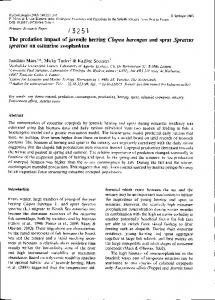
ies on the vertical and horizontal structure of pelagic fish schools over the 24-h relating DVM with feeding behaviour in the marine environment are, to our knowledge, scarce in the literature (e.g. Blaxter, 1985), limited to tank experiment (Sogard and Olla, 1996) and lacking for the Baltic Sea. Nevertheless, inferences on DVM of pelagic fish related to foraging may be done from lakes where DVM by zooplankton has been extensively studied (Levy, 1990a, b, 1991; De Stasio, 1993; Allison et al., 1996; Steinhart and Wurtsbaugh, 1999). Allison et al. (1996) showed peaks in feeding activity of pelagic fish (cichlids) at dawn and dusk in the Lake Malawi related to the DVM of their prey, i.e. zooplankton. Levy (1990b) and Stockwell and Johnson (1999) evaluated the relative importance of different factors explaining DVM of salmon in lakes arguing that a multifactor hypothesis (foraging, bioenergetics and predator avoidance) provided the most realistic explanation of the adaptive significance of DVM in pelagic fish. The Baltic Sea pelagic ecosystem is constituted by the top-piscivores cod (Gadus morhua) and the major pelagic planktivores, herring (Clupea harengus) and sprat (Sprattus sprattus). Nektobenthos is represented essentially by Mysis sp. while zooplankton is dominated by calanoid copepods, but cladocerans and rotifers can be abundant (Rudstam et al., 1994). Hansson et al. (1990) investigated DVM of zooplankton (occupying the deeper and darker water during the day and the upper water column in the night) in the Baltic Sea arguing that this phenomenon was essentially explainable by anti-predation behaviour. In this paper we investigated pelagic fish (herring and sprat) (a) horizontal movements at the temporal small-scale (data from 1995 survey), (b) DVM and degree of aggregation (data from 1995 survey) and (c) size distribution at different depth and time of the day and diel feeding pattern (data from 1997 survey). 2. Materials and methods 2.1. Surveys design and collection of data 2.1.1. Survey 1995 In October 1995 an acoustic survey was conducted onboard the Swedish research vessel “Argos” in an area south of the Bornholm depth in the southern part of the Baltic Sea (Fig. 1). The 1995 survey was used to estimate the diel spatial distribution of pelagic fish. Recordings of acoustic data of fish were made by SIMRAD EK400 and EK500 38 kHz split-beam echo-sounders. These data were supplemented with geographical position from Global Positioning System in terms of geographical co-ordinates (latitude and longitude). The echo integrator data were collected from 10 m below the sea surface (transducer at 8 m depth) to 1 m above the seabed. Data were recorded using the Simrad BI500 software package on a SUN Sparc IPC computer and stored on DAT tapes. The echo sounder provides a mean integrated value for each 0.1 nautical mile (nm; 1 nm = 1.852 km).
Fig. 1. Study area and sampling design during the 1995 survey. The survey quadrate, constituted by four transects (A–D), was ensonified four times each day (3, 4 and 11 October).
The area investigated was divided in four transects forming a survey quadrate of 15 nm per side (Fig. 1). The survey quadrate was ensonified four times during the 24-h (0–6, 6–12, 12–18, 18–24 h) with a standard vessel speed of 10 knots. The survey was conducted for 3 d on the 3, 4 and 11 October. During the experiment weather conditions were good with a stable high-pressure and variable wind, sunrise was at 05:00 UT (Universal Time) and sunset at 16:30 UT. All the hours mentioned in this study refer to UT. The moon was in its first increasing quarter. The area was chosen because of a high concentration of fish as estimated by the acoustic device. Profiles of water temperature (°C), salinity (psu) and oxygen (ml l–1) content were recorded at 0, 2.5, 5, 10, 15, 20, 30, 40, 50, 60, 70 and 80 m depth using a CTD (Conductivity Temperature Depth) probe. 2.1.2. Survey 1997 In the 1997 an acoustic survey was conducted onboard the Swedish research vessel “Argos” in the same area and in the same period of the year as in the 1995 survey (Fig. 1). The 1997 survey was conducted to estimate the diel feeding cycle of pelagic fish (herring and sprat) and analyse their species and size distribution by depth and time of the day. Individuals of herring and sprat were collected during the 24-h in 3 d using a pelagic trawl net. Fishing was performed with two different pelagic trawls (14–17 m vertical opening; 21 mm stretched mesh size in the cod-end). Size-selectivity of the two trawls used was not statistical different (Bethke et al., 1999). Standard fishing speed was 3–4.5 knots and hauls lasted for approximately 30 min (Bethke et al., 1999). Catches were sorted at species level and a sub-sample of
M. Cardinale et al. / Aquatic Living Resources 16 (2003) 283–292
300 herring and 200 sprat individuals for each haul was measured (total length) to the nearest 0.5 cm for lengthfrequency distribution analysis. Individual fish were immediately frozen onboard and then processed in the laboratory. A random sample of about 100 herring and 50 sprat for each haul was collected for feeding analysis. In the laboratory, each fish collected was measured (total length) to the nearest 0.5 cm and weighed to the nearest 0.1 g and the stomachs investigated for fullness. A simple approach to calculate feeding cycle in the field is to estimate the proportion of fish with food in the stomach during the 24-h. It simply requires an estimate of the percentage of empty stomachs randomly collected. The effort to collect the data is irrelevant in comparison with other models, particularly when dealing with big sample areas such as the marine environment (Bromley, 1994).
3. Statistical analysis 3.1. Survey 1995. Spatial distribution of fishes during the 24-h Processed Sa values were used as an index of fish abundance in the sea. In the southern Baltic Sea, herring and sprat constitutes more than 97% of the pelagic fish biomass (Orlowski, 2001). Therefore, the estimated Sa values were assumed to reflect essentially the biomass of herring and sprat and were used as an index of pelagic fish density in the sea. Sa values were transformed (Ln Sa valves + 1) to conform to assumptions of homogeneous variance, normality and linearity (Sokal and Rohlf, 1995). Data were divided into four depth strata (10–20, 21–40, 41–60, 61–80 m) and fish abundance at the different depth strata during the 24-h was compared using Variance Components Analysis and Factorial ANOVA in Statistica computer package (Statistica, 1995). HSD post-hoc tests (Sokal and Rohlf, 1995) were used for mean comparisons. To define changes in degrees of fish aggregation among different hours and depth strata we used the coefficient of variation (CV %) among point estimates of fish abundance as an index (Hilborn and Mangel, 1997). We assumed that when fish are dispersed the variance should be the lowest and when fish are highly aggregate the largest. 3.2. Survey 1997. Diel feeding cycle and species/size distribution of pelagic fish We estimated the length–frequency distributions of herring and sprat and the proportion of the two species in the catch during the day (05:30–16:30) and night (17:30–04:30) at the surface (10–40 m) and at the bottom (41–80 m). Kolmogorov-Smirnov tests (K-S test) (Sokal and Rohlf, 1995) were used to compare length–frequency distributions. The significance level was set at 5% for all the statistical tests used in the analyses.
285
Fig. 2. Depth profiles of temperature, salinity and oxygen content in the study area during the 1995 survey.
4. Results 4.1. Survey 1995. Spatial distribution of fishes during the 24-h Profiles of water temperature (°C), salinity (psu) and oxygen (ml l–1) content are shown in Fig. 2. A thermocline occurred between 30 and 50 m, salinity was between 5–6 psu down to 40 m and increased to 13 at 80 m depth. Oxygen values were comprised between 6 and 7 ml l–1 within 0–40 m decreasing to 0 ml l–1 at 70 m depth. Overall, distinct variability was observed in both the horizontal and vertical distribution of fish abundance in space and time. Variables ‘day’ and ‘survey quadrate’ and their first interaction term significantly contributed while variable ‘transect’ did not contribute to explain the total variance of fish abundance during the experiment (Table 1). Fish abundance was significantly different among days (HSD-test), although without a defined pattern (Fig. 3). An increase in fish abundance occurred between the first (October 3) and the second day (October 4) followed by a significant decrease (HSD test; P < 0.05) in the third day (October 11) in all the different transects except in D. Here the difference between the second and third day was not significant (HSD test; P > 0.05). Fish abundance differed significantly (Table 1) also between different survey quadrates among days and transects but without a well-defined trend during the 24-h (Fig. 3). The contribution of the variable ‘time’ to the total variance was not significant for any of the 3 d while ‘depth’ and ‘depth × time’ interaction term contributed significantly to the total variance (Table 1). Therefore, we used the 24-h as a single transect testing for diel differences in fish abundance at the different depth strata. Differences in fish abundance occurred among different depth strata during the 24-h (Table 1). Fishes were most abundant between 41 and 80 m (i.e. the deeper part of the thermocline) during the day (HSD test; P < 0.01). During the afternoon they migrated to the upper layer (10–40 m) and reached the largest values at the surface
286
M. Cardinale et al. / Aquatic Living Resources 16 (2003) 283–292
Table 1 Results of Variance Components Analysis and Factorial ANOVA of the 1995 acoustic survey data. d.f. = degrees of freedom; MS = mean square; P = probability level, ns (not significant) = P > 0.05. {n}·{nx}is the interaction factor between the different variables tested All days {1}day {2}survey quadrate {3} transect {1}·{2} {1}·{3} {2}·{3} {1}·{2}·{3}
d.f. effect 2 3 3 6 6 9 18
MS effect 54.9 17.4 5.3 2.9 8.4 2.6 1.0
d.f. error 8.0 9.2 8.0 18.6 18.0 18.0 6979.0
MS error 10.3 4.5 10.0 1.0 1.0 1.0 0.2
F 5.34 3.86 0.53 2.81 8.39 2.64 6.57
P