DART: Directional Anypath Routing in Wireless Mesh Networks Xi Fang Arizona State University
[email protected]
Dejun Yang Arizona State University
[email protected]
Abstract— Anypath routing is proposed to improve the performance of wireless networks by exploiting the spatial diversity and broadcast nature of the wireless medium. In this paper, we study anypath routing in wireless networks with directional antennas, and propose DART (Directional Anypath RouTing), a crosslayer design of MAC and routing layers. For the routing layer, we propose two shortest directional anypath routing algorithms based on two antenna models. Our routing algorithms are simple and fast, thus are suitable for implementation in practical protocols. For the MAC layer, we present a directional anycast MAC, which is an enhancement to the IEEE 802.11 MAC, making DART suitable for integration into current systems. Simulation results show that DART can significantly reduce the packet transmission delay.
Guoliang Xue Arizona State University
[email protected]
forwarder actually forwards the packet, every packet from the source 𝑠 traverses only one of the available paths to reach the destination 𝑡. The dashed red line in Fig.1 shows a possible path of a data packet. Different packets might take different paths. Therefore, paths are determined on-the-fly, depending on which forwarders receive the packet at each hop. The anypath shown in Fig.1 is composed of six different paths. 0.3
v1 0.2
v4
1
s
0.1
0.7 0.5
v3
t
1
I. Introduction In unreliable wireless networks, due to the broadcast nature of wireless medium, it is usually less costly to transmit packets to any node in a set of neighbors than to one specific neighbor [9]. This observation motivates a novel technique known as opportunistic routing, which can significantly improve the performance of wireless networks [2, 3, 9, 16]. [2] designed an opportunistic routing protocol ExOR, and [3] proposed MORE by integrating network coding into OR. [9] introduced anypath routing, which was subsequently studied in [10, 16]. In anypath routing, each packet is broadcast to any node in a forwarding set composed of one or more neighbors (called forwarders) instead of to one specific neighbor. The packet is retransmitted if and only if none of these neighbors receives it. Such broadcast is usually called anycast. As long as one of them receives this packet, it can be forwarded on. The forwarders of a node are each given a priority in relaying the received packet. Higher priorities are assigned to the forwarders with shorter distances to the destination. A forwarder forwards a packet only when all the higher priority forwarders fail to receive it. For each packet, the source keeps rebroadcasting it until some forwarders receive it or a threshold is reached. Once a forwarder receives the packet, it will repeat the same procedure above until this packet is successfully delivered to the destination. An anypath from a source to a destination is a directed graph where every node (but the source) is a successor of the source, and every node (but the destination) is a predecessor of the destination. We use Fig.1 to illustrate an anypath. Ignore the edge weights and the colored sectors for the moment, which are explained in Section II. An anypath is shown in bold arrows. For instance, 𝑠, 𝑣1 and 𝑣2 have forwarders {𝑣1 , 𝑣2 }, {𝑣3 } and {𝑣3 , 𝑣6 }, respectively. Since at every hop only one This research was supported in part by NSF grants 0830739 and 0905603. The information reported here does not reflect the position or the policy of the federal government.
0.5
v2
1 0.1
0.1
v6
0.1
0.2
v5
Fig. 1. Illustration of anypaths. The edge weight denotes its packet delivery ratio. The sector on each node represents its forwarding sector.
s
v1 v2
Fig. 2.
v3
t v4
A motivating example of directional anypath routing.
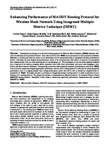
Prior works along this line mainly focused on networks equipped with omnidirectional antennas. However, [24] proved that wireless networks can achieve a capacity gain when directional antennas are exploited. [4, 12, 18, 20, 22, 23] have proposed various schemes to improve performance of wireless networks by using directional communications. Thus it is of interest to design an optimally combined use of directional communications and anypath routing. Let us consider a motivating example shown in Fig. 2. 𝑠, 𝑣1 , 𝑣2 and 𝑣3 ’s forwarding sets are {𝑣1 , 𝑣2 }, {𝑡, 𝑣4 }, {𝑣3 } and {𝑣1 }, respectively. Obviously, if the directional transmission range of 𝑣1 just covers 𝑡 and 𝑣4 as shown in Fig. 2, it will not interfere with the transmission from 𝑣2 to 𝑣3 , and thus the delay from 𝑣2 to 𝑣3 is reduced. Although [17] touched on the opportunistic routing with directional antennas, it is based on the node distribution models and cannot compute an actual anypath for a source-destination pair in a wireless network. In order to bridge this gap, in this paper we study anypath routing for wireless networks equipped with directional antennas. From the perspective of the MAC layer, the challenge is how to realize directional anycast with relay priority guaranteed. A reliable anycast MAC even in the omnidirectional antenna system is an active area of research [5, 14, 15]. From the perspective of the routing layer, looking for an optimal
II. System Model and Problem Formulation A. Antenna Model The antenna system has two separate modes: Directional and Omni, which could be envisioned as two separate antennas: a steerable single beam antenna and an omnidirectional antenna[4]. The boresight of the main lobe can be pointed towards any specified direction in the Directional mode. This kind of antennas is called electrically steerable antenna [4, 12, 19, 22, 23]. According to [19], a typical beam switching latency is about 150𝜇𝑠. In principle, both the Directional and the Omni modes can be used to transmit or receive packets. As in [4], the Omni mode in this paper is used for reception, while the Directional mode may be used for transmission as well as reception. While idle (i.e. not transmitting or receiving) a node stays in the Omni mode. This kind of antenna can be implemented by integrating directional transmitters and omni/directional receivers [6]. The main lobe in the Directional mode is approximated as a circular sector with radius 𝑟, called transmission range (i.e. the yellow area in Fig.3), where 𝔸𝑠 and 𝔸𝑒 denote the start and end angles of the sector (measured counterclockwise from the horizontal axis), and 𝔸𝑏 denotes its beamwidth. The line segments 𝐿𝑠 and 𝐿𝑒 are called the start and end boundaries. All the points in this transmission range with the same distance from the center have the same directional transmission gain. The radiation pattern of the side lobes is also approximated as a sector. The gain of the side lobes is assumed to be very
low, and is thus negligible. Note that this approximation is widely used in the literature [4, 17, 22, 24], and is often called ideal directional antenna model. For the beamwidth in the Directional mode, we consider two models. In the fixed beamwidth model [12, 20], the beamwidth of each transmitter is fixed although different antennas can use different beamwidths. In the variable beamwidth model [17, 18, 20], each transmitter has an adjustable beamwidth 𝔸𝑏 ∈ [𝐴𝑙 , 𝐴𝑢 ], where 0 0. We will describe how to measure PDR using probes in Section III.B. Since a busy link may cause a probe broadcast to be deferred, but ordinarily does not cause it to be lost [8], we assume that the average PDR of edge (𝑣, 𝑢) is constant if the directional transmission gain of 𝑣 at 𝑢 does not change. This implies that we can steer the boresight or adjust the beamwidth of a transmitter without changing the PDRs of the edges in 𝐺. Thus PDR 𝑝(𝑣, 𝑢) can be considered as a constant property of each edge for routing computation. Note that this assumption holds for the ideal directional antenna model (see Section II-A). However, this assumption may not hold for some real antenna implementations. Consider two locations with the same distance far away from a directional antenna. The gain at the location close to the boundary of the transmission range may be smaller than the gain at the location close to the boresight. For a real directional antenna, if it satisfies that the obtained gain drops quickly when a location is approaching the boundary, the ideal directional antenna is a good approximate for such real direction antenna. The hyperlink delivery ratio 𝑝(𝑣, 𝐹 ) is defined as a measured probability that a packet sent by node 𝑣 is received by at least one of the nodes in forwarding set 𝐹 . Since [16] indicates that the loss of a packet at different receivers occurs independently, it can be computed as 𝑝(𝑣, 𝐹 ) = 1 − ∏ (1 − 𝑝(𝑣, 𝑢)). 𝑢∈𝐹 In directional anypath routing, each node is equipped with an antenna system following the antenna model in Section II.A. Each transmitter has a steerable transmission range, called forwarding sector. The forwarders of a node must be in its forwarding sector. We use 𝐹 ∈ Λ to indicate that forwarding set 𝐹 is located in the forwarding sector Λ. Fig.1 illustrates this concept. The directional anypath is still shown in bold arrows. The forwarding sector of each node is also shown. All the forwarders of a node must be located in its forwarding sector. In brief, compared with traditional anypath routing, each node should choose both its forwarding sector (boresight and beamwidth) and the forwarding set of this forwarding sector rather than just forwarding set. Now we are ready to define the directional anypath distance (DAD) based on PDR. We will discuss the effectiveness of this PDR-based metric in Section II.C. The distance 𝑑(𝑣, 𝐹 ) 1 from node 𝑣 to a set of nodes 𝐹 is defined as 𝑝(𝑣,𝐹 ) , which represents the expected number of transmissions for a packet sent by 𝑣 to be received by at least one node in 𝐹 . The DAD from 𝑣 to 𝑡 along a directional anypath is recursively defined as: 𝔻(𝑣) = min (𝔻𝐹 (𝑣)) = min (𝑑(𝑣, 𝐹 ) + 𝔻(𝐹 )), (1) 𝐹 ∈Λ
𝐹 ∈Λ
where Λ is the forwarding sector of 𝑣, 𝔻𝐹 (𝑣) = 𝑑(𝑣, 𝐹 ) + 𝔻(𝐹 ) is the anypath distance of 𝑣 via forwarding set 𝐹 , and 𝔻(𝐹 ) is the remaining DAD from 𝐹 to the destination. It is intuitively defined as a weighed average of the DADs from
the nodes in the forwarding set 𝐹 to the destination: ∑ 𝛼(𝑢𝛽 )𝔻(𝑢𝛽 ), 𝔻(𝐹 ) =
(2)
𝑢𝛽 ∈𝐹
∑ with 𝑢𝛽 ∈𝐹 𝛼(𝑢𝛽 ) = 1, where the coefficient 𝛼(𝑢𝛽 ) represents the probability of a node with priority 𝛽 ∈ [1, ∣𝐹 ∣] forwarding a received packet. The value of the node priority (i.e. 𝛽) is called its priority index. For example, the highest priority node 𝑢1 has priority index 1.Thus, a forwarder with a larger DAD should have a lower priority or a larger priority index [9]. Obviously, a node with priority 𝛽 forwards a packet only when it receives this packet and none of the higher priority ∏ nodes receives it, which happens with probability 𝛽−1 𝑝(𝑣, 𝑢𝛽 ) 𝑞=1 (1 − 𝑝(𝑣, 𝑢𝑞 )).Thus 𝛼(𝑢𝛽 ) can be computed as ∏𝛽−1 ∏𝛽−1 𝑝(𝑣, 𝑢𝛽 ) 𝑞=1(1−𝑝(𝑣, 𝑢𝑞 )) 𝑝(𝑣, 𝑢𝛽 ) 𝑞=1(1−𝑝(𝑣, 𝑢𝑞 )) = , 𝛼(𝑢𝛽 )= ∏∣𝐹 ∣ 𝑝(𝑣, 𝐹 ) 1 − 𝑞=1 (1 − 𝑝(𝑣, 𝑢𝑞 )) with the denominator being the normalizing constant. Obviously, according to this definition, 𝔻(𝑣) represents the expected total number of transmissions necessary for a packet sent by 𝑣 to be received by destination 𝑡 along this directional anypath. The forwarding set in Λ, which can provide the minimum 𝔻𝐹 (𝑣), is called the optimal forwarding set of Λ. As an example, consider the network depicted in Fig. 1 to compute 𝔻(𝑣3 ). The forwarding sectors of 𝑣3 and 𝑣5 are shown as the two sectors. The anypath distance from 𝑣3 to 𝑡 via the forwarding set 𝐹 = {𝑡, 𝑣5 } (note that 𝑡 and 𝑣5 are located in the forwarding sector of 𝑣3 ) is calculated as 𝔻𝐹 (𝑣3 ) = 𝑑(𝑣3 , 𝐹 ) + 𝔻(𝐹 ) 1 +0) 0.5 ×0+(1− 0.5) ×1×( 0.2 1 + =3.5. = 1−(1 − 0.5)(1 − 1) 1 − (1 − 0.5)(1 − 1) Note that 𝑡 can be considered as a forwarder with DAD 0, and 1 that the DAD of 𝑣5 is calculated as ( 0.2 + 0). Likewise, we can compute 𝔻{𝑣5 } (𝑣3 ) = 6 and 𝔻{𝑡} (𝑣3 ) = 2. Thus, 𝔻(𝑣3 ) = min{2, 3.5, 6} = 2, and {𝑡} is the optimal forwarding set of 𝑣3 ’s current forwarding sector. As explained in [9, 16], adding an extra node to the forwarding set is not always beneficial even if it reduces the forwarding delay from a node to any of its forwarders. For instance, clearly the anypath distance of 𝑣3 via {𝑡} is smaller than that via {𝑡, 𝑣5 }. Remark: Note that the above routing metric does not consider boresight or beamwidth adjustment delay. This is because we consider the routing metric from the perspective of the number of transmissions. In an unreliable wireless environment, compared with the total transmission time (including retransmission time) of a packet, the boresight or beamwidth adjustment delay is usually much smaller. Therefore, our routing metric does not consider boresight or beamwidth adjustment delay. C. Problem Formulation MAC layer: For directional anycast, the MAC should address the following issues. 1) It must solve directional transmissions, interference, collisions and the corresponding scheduling problems existing in a directional antenna system. 2) It must realize anycast with relay priority guaranteed.
3) It must know whether a packet has been delivered to one of its forwarders, and when to retransmit if failed. 4) It must consider the compatibility with the currently existing wireless networks (such as 802.11 networks). Routing layer: Routing layer aims to find a shortest directional anypath from a source to a destination. We need to point out that the shortest directional anypath defined on PDR may not be the real optimal one for a certain packet transmission since the metric PDR cannot reflect the actual reduction on interference when directional antenna is being used. However as discussed in Section II.B, we remark that this formulation is a practical and helpful approximation, largely due to the undetermined load pattern and probabilistic nature of lossy wireless networks. We study two versions of the routing problem based on the two beamwidth models described in Section II.A. The first version is the fixed beamwidth shortest directional anypath routing (FBDAR). Finding a shortest directional anypath is equivalent to finding an optimal forwarding sector for each node, which can provide the shortest DAD, and the optimal forwarding set of this forwarding sector. Note that since the beamwidth is fixed for each node, we only need to determine the boresight of the optimal forwarding sector for each node. The second version is the variable beamwidth shortest directional anypath routing (VBDAR). Similar to FBDAR, we need to find an optimal forwarding sector and the optimal forwarding set of this forwarding sector for each node. Note that in this version the optimal forwarding sector refers to the one with the minimum beamwidth among all the forwarding sectors which can provide the shortest DAD. III. DART MAC Layer Design In this section, we present a MAC design to support the practical implementation of DART. A. Directional Anycast MAC We present DAM, a directional anycast MAC, which is an enhancement to the 802.11 MAC [13]. A similar handshaking scheme (i.e. RTS/CTS/DATA/ACK [13]) is used in DAM. We use a directional network allocation vector (DNAV) [4] to keep track of the directions (and the corresponding durations) towards which a node must not initiate a transmission. The well-known network allocation vector (NAV) used in 802.11 indicates the duration for which the node must defer transmission to avoid interfering with some other transmission. The difference between DNAV and NAV is that if a node receivers an RTS/CTS from a certain direction, it needs to defer only those transmissions that are directed in that direction. The entry in DNAV is updated based on the “duration” field and the incoming direction of the overheard packets. When the routing layer passes a packet and the information about forwarders to DAM, DAM requests the physical layer to beamform to the forwarding set, and performs carrier sensing for at least a DIFS (defined in 802.11 [13]) to detect whether the channel is idle. Carrier sensing is performed by both physical and virtual mechanisms. Virtual carrier sensing is performed based on DNAV. More specifically, if node 𝑢 has a packet to send to 𝑣, it must check its DNAV table to decide if it
is safe to transmit in the direction of 𝑣. If idle, DAM enters the backoff phase as in 802.11. Once its backoff counter counts down to zero, the transmitter will broadcast directionally to these forwarders an RTS (called MRTS) with all the forwarder addresses (ordered according to their priorities). If the medium is busy, the transmitter waits until it becomes idle. Recall that all the idle nodes stay in the Omni mode. Once they receive a signal arriving from a particular direction, they lock on to this direction and receive it. If an intended forwarder receives the MRTS packet, it responds by a CTS directionally. However, these CTS transmissions must be staggered in time in order of their priorities. The highest priority forwarder replies the CTS after an SIFS (defined in [13]), the second one replies after (CTS+3×SIFS) time, the third one after (2×CTS+5×SIFS) time and so on. When the transmitter receives a CTS, it directionally sends the DATA to the sender of this CTS after an SIFS interval. This can guarantee that the lower priority forwarders hear this DATA before they transmit CTSs, thus they suppress any further CTS transmissions. This is the key point to enforce the prioritization among forwarders. All such forwarders set their DNAVs (i.e. this direction is busy) until the end of the ACK period, and switch back to Omni mode. Note that it is possible that an intended forwarder has locked on to another direction, and is thus “deaf” to this MRTS. DAM does not require all the intended forwarders to be idle when a node is trying to send an MRTS. The “deafness” will be discussed in Section III.B. If DATA is successfully received, this forwarder replies an ACK directionally. In practice the channel status could change from the point when CTS is transmitted to the point when DATA or ACK is transmitted, which causes the exchange to fail. However, [14] proves that the probability is low, since for static or slowly changing dynamic wireless networks the coherence period is expected to be large enough for the DATA transmission to succeed, if the transmissions of RTS and CTS are indeed successful. If the DATA transmission fails indeed (i.e. ACK-timeout), DAM just repeats the whole procedure (i.e. MRTS/CTS/DATA/ACK). Any other node that overhears the MRTS or the DATA (i.e. exposed node) sets its DNAV for the entire duration specified in the MRTS or DATA. Specifically, if the MRTS is received, the DNAV is set to (𝑘×CTS+(2𝑘 + 1)×SIFS+DATA+ACK) time, where 𝑘 is the number of forwarders. If the header of the DATA is received, the DNAV is set to (SIFS+DATA+ACK) time. Likewise, any node that overhears any of the CTSs (i.e. hidden node) sets its DNAV until the ACK period. That is to say, a node upon receiving the 𝑖-th CTS, must set its DNAV to ((2(𝑘 − 𝑖) + 1)×SIFS+(𝑘 − 𝑖)×CTS+DATA+ACK) time. If no CTS comes back within a CTS-timeout duration, the transmitter’s DAM will increase its contention window (if the maximum has not been reached), enter the backoff phase as in 802.11, and schedule a retransmission of the MRTS. Note that DAM actually slightly deviates from the basic operations of anypath routing in [9]. [9] requires some forwarders to suppress redundant forwardings. DAM realizes this by suppressing redundant CTS replies to guarantee that only
V1 V6
V2 V3
V1
V6
V2 V3
V1 V5
V5
V4
V4
(a) MRTS
(b) CTS
V6
V2
V6
V3
V1
V1
V2 V3
V5
V5
V4
V4
(c) DATA
(d) ACK
header
Transmitter
DIFS
MRTS
V2
Forwarder
V3
Forwarder
V4
Forwarder
V5 V6
SIFS
D DATA
SIFS+CTS 2*SIFS
CTS
SIFS
ACK
DNAV DNAV DNAV
(e) Timeline showing a successful directional anycast
Fig. 4. Illustration of the basic operation of DAM: suppose that currently the channel between 𝑣1 and 𝑣2 is bad; (a)𝑣1 broadcasts an MRTS to 𝑣2 (first highest relay priority), 𝑣3 (second highest relay priority) and 𝑣4 (third highest relay priority); the MRTS is heard by 𝑣3 , 𝑣4 and 𝑣5 ; 𝑣5 sets its DNAV and thus will not initiate a transmission towards the direction of 𝑣1 ; (b) since 𝑣2 (with the highest relay priority) does not receive the MRTS, 𝑣3 replies a CTS directionally after waiting for (3×SIFS+CTS) time; 𝑣3 ’s CTS is heard by 𝑣1 and 𝑣6 ; 𝑣6 sets its DNAV and thus will not initiate a transmission towards the direction of 𝑣3 ; (c) 𝑣1 starts transmitting data directionally to 𝑣3 ; 𝑣3 locks on to the direction of 𝑣1 and receives DATA; after having received the header of the DATA, 𝑣4 suppresses its CTS reply, sets DNAV and thus will not initiate a transmission towards the direction of 𝑣1 ; (d) once the DATA is successfully received, 𝑣3 replies an ACK directionally.
one forwarder will be responsible for forwarding this packet. We use Fig.4 to illustrate the basic operation of DAM. Suppose that 𝑣1 has three forwarders 𝑣2 , 𝑣3 , and 𝑣4 . 𝑣2 has the highest relay priority, 𝑣3 has the second highest one, and 𝑣4 has the lowest one. 𝑣1 performs both physical and virtual carrier sensing for at least a DIFS to detect whether the channel is idle. Once it finds the channel is idle, it broadcasts an MRTS directionally to its forwarders 𝑣2 , 𝑣3 , and 𝑣4 (see Fig.4(a)). Suppose that currently the channel between 𝑣1 and 𝑣2 is bad. Thus 𝑣2 , who has the highest relay priority, does not receive the MRTS from 𝑣1 . However, 𝑣3 , 𝑣4 and 𝑣5 receive this MRTS. Since 𝑣5 is not the intended forwarder, it sets its DNAV and thus will not initiate a transmission towards the direction of 𝑣1 until the ACK period (see Fig.4(e)). 𝑣3 waits for (CTS+3×SIFS) time (see Fig.4(e)), and replies a CTS directionally (see Fig.4(b)). Suppose that both 𝑣1 and 𝑣6 receive this CTS. Thus, 𝑣6 sets its DNAV and will not initiate a transmission towards the direction of 𝑣3 until the ACK period (see Fig.4(e)), and 𝑣1 starts to transmit DATA directionally to 𝑣3 (see Fig.4(c)). After having received the header of the DATA, 𝑣4 suppresses its CTS reply and sets its DNAV (see Fig.4(e)). When the DATA is received, 𝑣3 replies an ACK directionally (see Fig.4(d)). Therefore, a successful priority-enforced directional anycast is done. B. Practical Issues PDR measurement: Although we suggest using the traditional PDR [8] as our routing metric, considering that only the Directional mode is used for transmission, we slightly modify its operation for adapting to DART. In order to measure the average PDR, each transmitter keeps track of actually used beamwidths, and uses the moving average as the antenna beamwidth (if the beamwidth is adjustable) when it is measuring PDRs. In addition, each transmitter selects several measure directions with directional transmission ranges covering the whole 360∘ area, and broadcasts dedicated link probe packets directionally and periodically if this direction is not busy. Every node remembers the probes it receives during the last several seconds and calculates the PDR [8]. Dynamic networks and route computation: We mainly consider static or slowly changing dynamic mesh networks and thus use centralized routing algorithms. In other word, network topology and link status are assumed to be static. The
MAC of each node periodically measures PDRs, and keeps certain neighborhood status information dynamically. This status information from each node is propagated periodically through the whole network. This helps each node have the approximate knowledge of the network status periodically, and thus each node can adaptively compute an anypath towards destinations. Note that in a highly dynamic network nodes could have inconsistent knowledges about network topology and link PDRs. In this case, we may need a distributed routing algorithm. In Section VII, we describe a promising way to decentralize the routing algorithm. A more detailed design is our future work. Location information: Each node can use the Angle of Arrival technique [23] or the Direction of Arrival technique [4] to estimate the relative angle between each of its neighbors and itself based on a virtual axis. We will see that this relative angle information is enough for our routing algorithms. Scheduling: Since DAM is an enhancement to the 802.11 MAC, for the medium access, DART respects the 802.11 Distributed Coordination Function (DCF) [13]. For the problem of deciding which forwarder should be scheduled to receive the packet, DAM utilizes MRTS broadcasts and prioritized CTS replies. DAM does not require all the intended forwarders to be idle when it is trying to send an MRTS to fully utilize transmission opportunities if the transmission is safe. Compatibility with existing wireless networks: Our DAM reduces to the Basic Directional MAC protocol in [4] to some extent when there is only one forwarder for each node, and further reduces to 802.11 if only Omni mode is allowed. Deafness (or failed carrier sense) problems: DAM could suffer from deafness. Note that these issues also exist in other directional MACs, such as [4]. How to completely solve these issues is out of the scope of this paper. In addition, during the switching between omni and directional mode, the node cannot perform carrier sense and thus may transmit and interfere with other nodes’ transmissions. If these transmissions fail due to this interference, DAM just repeats the whole procedure (i.e. MRTS/CTS/DATA/ACK). Considering the duration of the switching operation between omni and directional mode is short, this case does not occur too frequently.
100
100
100
100
v1
v1
v1
v1
v1
t
10.4
s
2 0.1
0.5
v2
0. 9
0. 9
0 0.5
0
10.4
t
s
2 0.1
v2
5 0.
10
10
10
10
v3
v3
v3
v3
(b) 𝑡 is settled
(c) 𝑣2 is settled
(d) 𝑣3 is settled
0 0.5
t
0. 1
v2
1
2 0.1
0.
s
1
12
t
0.
0
1
0.5
5 0.
0.
v2
5 0.
(a) An example network
2 0.1
5
v3
s
0.
5 0.
∞
∞
0.
t
0. 9
0. 9
0 0.5
1
v2
01 0.
∞
01 0.
0.1
01 0.
s
01 0.
∞
01 0.
0. 9
∞
(e) 𝑠 is settled
Fig. 5. Algorithm illustration: the weight on each link denotes its PDR. The weight associated with each node denotes its currently computed shortest DAD 𝔻(𝑣). The sectors associated with each node denote its forwarding sectors in its ℝ(𝑣).
IV. DART Routing Algorithm for FBDAR In this section we present an efficient algorithm F-DART for FBDAR, which computes a shortest directional anypath from each node to the given destination 𝑡. From a high-level perspective, this algorithm is a Dijkstralike algorithm. However, as we study directional anypath routing, we need to use the formulas given in Section II to update distances and the corresponding data structures. For each node 𝑣 ∈ 𝑉 , we keep a variable 𝔻(𝑣) to store the currently computed shortest DAD from 𝑣 to 𝑡. Let 𝔸𝑠 (𝑣) and 𝔽(𝑣) denote the start angle of the corresponding forwarding sector and the corresponding forwarding set of this forwarding sector. Recall that in FBDAR for each node, its beamwidth is its property and known as a fixed number. Therefore, the start angle can uniquely determine the boresight of its forwarding sector. We use a list ℝ(𝑣) to keep track of all the candidate forwarding sectors for 𝑣. Each element (called a record) in ℝ(𝑣) keeps the corresponding information of this forwarding sector, including a set 𝐹 and two variables 𝐴𝑠 and 𝐷, which denote its forwarding set, its start angle and the anypath distance of 𝑣 via this forwarding set, respectively. Additionally, we keep two data structures: 𝐿 and 𝑄. 𝐿 is a list that stores all the settled nodes for which we have already found the shortest directional anypaths. We store all the other nodes in a priority queue 𝑄 keyed by their current 𝔻(𝑣) values. Now we briefly describe how Algorithm 1 works using the example shown in Fig.5. Suppose that the beamwidths of 𝑠, 𝑣1 and 𝑣2 are 90∘ , and the beamwidth of 𝑣3 is 30∘ . Lines 13 initialize all the data structures, and set 𝔻(𝑡) to 0. In the main while-loop, each time Line 5 extracts from 𝑄 a node with the minimum 𝔻, and inserts it into 𝐿. If its 𝔻 is ∞ already, all the nodes still in 𝑄 cannot reach the destination 𝑡 and thus the algorithm terminates. In the first iteration, 𝑡 is extracted in Line 5. Lines 7-14 then perform relaxations for all its incoming neighbors 𝑣1 , 𝑣2 and 𝑣3 . We take 𝑣2 as an example. Since now for 𝑣2 , its ℝ(𝑣2 ) is empty, Lines 8-12 are skipped. Line 13 constructs a forwarding sector for 𝑣2 (as shown in Fig.5(b)), and a corresponding record which stores the information of this forwarding sector. Note that now 𝑡 is added into the forwarding set associated with this forwarding sector since 𝑡 is the only settled outgoing neighbor located in it. Then for 𝑣2 , Line 14 updates the corresponding data structures by choosing the one which can provide the shortest DAD among all the constructed records (note that now 𝑣2 has
Algorithm 1 F-DART 1: for each node 𝑣 in 𝑉 do 2: 𝔻(𝑣) ← ∞, 𝔸𝑠 (𝑣) ← 0, 𝔽(𝑣) ← ∅, ℝ(𝑣) ← ∅. 3: 𝔻(𝑡) ← 0, 𝐿 ← ∅, 𝑄 ← 𝑉 . 4: while 𝑄 ∕= ∅ do 5: 𝑢 ← Extract-Min(𝑄), 𝐿 ← 𝐿 ∪ {𝑢}. 6: if 𝔻(𝑢) = ∞ then break. 7: for each unsettled incoming neighbor 𝑣 do 8: for each record 𝑅 in ℝ(𝑣) do 9: if 𝑢 is in the forwarding sector of 𝑅 then 1 10: 𝐹 ← 𝑅.𝐹 ∪ {𝑢}, 𝐷 ← 𝑝(𝑣,𝐹 ) + 𝔻(𝐹 ). 11: if 𝐷 < 𝑅.𝐷 then 12: 𝑅.𝐹 ← 𝐹 , 𝑅.𝐷 ← 𝐷. 13: Construct a record 𝑅𝑐 for 𝑣 such that 𝑢 is on the start boundary of the forwarding sector of 𝑅𝑐 . Set 𝑅𝑐 .𝐹 to the set of all the settled outgoing neighbors located in this forwarding sector. Calculate 𝑅𝑐 .𝐷. 14: 𝔻(𝑣) ← min 𝑅.𝐷, 𝔸𝑠 (𝑣) ← arg min 𝑅.𝐴𝑠 , 𝑅∈ℝ(𝑣)
𝔽(𝑣) ← arg min 𝑅.𝐹 ; update 𝑄.
𝑅.𝐷
𝑅.𝐷
only one record). Thus its currently computed shortest DAD is 2. Similar relaxations are performed on 𝑣1 and 𝑣3 , and their currently computed shortest DADs are updated to 100 and 10, respectively. In the second iteration, 𝑣2 is extracted in Line 5 since its 𝔻(𝑣2 ) is the smallest among all the unsettled nodes. Algorithm 1 repeats the similar procedure, relaxes its incoming neighbor 𝑠 and constructs the first record for 𝑠 (as shown in Fig.5(c)) with the forwarding set {𝑣2 } (since 𝑣2 is the only settled outgoing neighbor located in it.). In the third iteration, 𝑣3 is extracted, and Lines 7-14 perform relaxations for its incoming neighbor 𝑠. Note that now ℝ(𝑠) is not empty. Lines 8-12 check for the first forwarding sector (the yellow one) in ℝ(𝑠) whether 𝑣3 is located in it. Since this forwarding sector only has 𝑣2 in it, and 𝑣3 is not located in it, this if-branch is skipped. Then Line 13 constructs the second forwarding sector for 𝑠 (the green one) as shown in Fig.5(d), and sets its forwarding set of this record to the set of all the settled outgoing neighbors located in this forwarding sector (i.e. 𝑣2 and 𝑣3 ). Since the second record leads to a smaller DAD, Line 14 chooses this forwarding sector and updates the corresponding data structure. As shown in Fig.5(e), in the
fourth iteration 𝑠 is extracted and thus settled. Theorem 4.1: Algorithm 1 finds a shortest directional anypath for FBDAR in 𝑂 (∣𝐸∣ (log ∣𝑉 ∣ + Δ(𝐺) log Δ(𝐺))) time, where Δ(𝐺) is the maximum out-degree of graph 𝐺. □ We need to give Lemmas 4.1-4.5 before proving Theorem 4.1. Let 𝜃(𝑣) denote the optimal DAD of 𝑣. Note that Lemmas 4.1-4.3 are similar to Lemmas 4.1-4.3 in [10], which studied multi-constrained anypath routing. We can use similar techniques in [10] to prove Lemmas 4.1-4.3. Due to the space limit, we omit the proofs for these three lemmas. Lemma 4.1: If the forwarders of node 𝑣 can only be chosen from a nonempty subset of its outgoing neighbor nodes, denoted by 𝑁 (𝑣) = {𝑢1 , 𝑢2 , . . . , 𝑢𝑧 } (with 𝜃(𝑢1 ) ≤ 𝜃(𝑢2 ) ≤ ⋅ ⋅ ⋅ ≤ 𝜃(𝑢𝑧 )), there must exist an optimal forwarding set of the form {𝑢1 , 𝑢2 , . . . , 𝑢𝑏 } for some 𝑏 ∈ {1, 2, . . . , 𝑧}, called a full optimal forwarding set (FOFS) in 𝑁 (𝑣) for node 𝑣. □ Suppose that there are four optimal forwarding sets in 𝑁 (𝑣) for node 𝑣: {𝑢1 , 𝑢2 }, {𝑢1 , 𝑢2 , 𝑢3 }, {𝑢1 , 𝑢2 , 𝑢3 , 𝑢4 }, and {𝑢1 , 𝑢2 , 𝑢4 }. This could happen, for example, when 𝑝(𝑣, 𝑢2 ) = 1. We can easily verify that these three forwarding sets lead to the same DAD. {𝑢1 , 𝑢2 }, {𝑢1 , 𝑢2 , 𝑢3 }, {𝑢1 , 𝑢2 , 𝑢3 , 𝑢4 } are FOFSs. Recall that a node’s forwarders must be located in its forwarding sector. Once the forwarding sector is determined, the set of nodes, from which we choose forwarders, is therefore determined. Let 𝑁 (𝑣) = {𝑢1 , 𝑢2 , ..., 𝑢𝑧 } denote the set of these nodes. Lemma 4.1 implies that we only need to check forwarding sets {𝑢1 }, {𝑢1 , 𝑢2 }, .... Thus the time complexity of finding the optimal forwarding set of a forwarding sector can be reduced to a polynomial time from an exponential time. The proof of Lemma 4.1 will construct such an FOFS (refer to the proof of Lemma 4.1 in [10]) that among all the optimal forwarding sets in 𝑁 (𝑣), the largest priority index node in this FOFS has the smallest priority index. Thus, if we check the forwarding sets in this order {𝑢1 }, {𝑢1 , 𝑢2 }, ..., this constructed FOFS would be found earliest among all the optimal forwarding sets in 𝑁 (𝑣). We call this FOFS a minimum FOFS (MFOFS) in 𝑁 (𝑣). Consider the example above. We have three FOFSs {𝑢1 , 𝑢2 }, {𝑢1 , 𝑢2 , 𝑢3 }, and {𝑢1 , 𝑢2 , 𝑢3 , 𝑢4 }. The MFOFS is {𝑢1 , 𝑢2 }, since the priority index of the largest priority index node in {𝑢1 , 𝑢2 } is 2, which is smaller than 3 in {𝑢1 , 𝑢2 , 𝑢3 }, and 4 in {𝑢1 , 𝑢2 , 𝑢3 , 𝑢4 }. However, since there are an infinite number of possible boresights of the forwarding sector, we may ask which is the optimal. Lemma 4.4 will show that we only need to check a polynomial number of boresights. We call the MFOFS of the optimal forwarding sector an optimal MFOFS (OMFOFS). For example, we have two forwarding sectors available. The MFOFS in the first one leads to a DAD of 5, while the MFOFS in the second one leads to a DAD of 10. The MFOFS in the first one is an OMFOFS. If all the nodes on a shortest (i.e. optimal) directional anypath from 𝑣 to 𝑡 use their OMFOFSs, we call it a full shortest anypath or a full optimal anypath. Lemma 4.2: For an arbitrary nonempty subset 𝑁 (𝑣)={𝑢1 , 𝑢2 , . . . , 𝑢𝑧 } of the outgoing neighbors of a node 𝑣, its MFOFS is {𝑢1 , 𝑢2 , . . . , 𝑢𝑏 } with optimal distances 𝜃(𝑢1 ) ≤ 𝜃(𝑢2 ) ≤
⋅ ⋅ ⋅ ≤ 𝜃(𝑢𝑏 ). Let 𝑆𝜇 denote the set {𝑢1 , 𝑢2 , . . . , 𝑢𝜇 }, 1 ≤ 𝜇 ≤ 𝑏. Then we have 𝔻𝑆1 (𝑣) > 𝔻𝑆2 (𝑣) > ⋅ ⋅ ⋅ > 𝔻𝑆𝑏 (𝑣). □ Lemma 4.3: The optimal DAD 𝜃(𝑣) of a node 𝑣 is always larger than that of any node (other than 𝑣) on the full shortest anypath from node 𝑣 to destination 𝑡. □ Lemma 4.4: Let Δ(𝑣) denote the out-degree of node 𝑣 in 𝐺. Although there exist an infinite number of possible forwarding sectors for 𝑣, in order to find the optimal one, it is sufficient to check 𝑂(Δ(𝑣)) particular forwarding sectors. □ Proof. We construct the 𝑂(Δ(𝑣)) forwarding sectors for 𝑣 as follows. For each outgoing neighbor node of 𝑣, we construct a forwarding sector of 𝑣 such that this node is on its start boundary. We can therefore construct 𝑂(Δ(𝑣)) forwarding sectors, called forwarding sector candidates. We now consider an arbitrary forwarding sector Λ′ of 𝑣, and prove that the DAD of 𝑣 via Λ′ cannot be smaller than that via one particular forwarding sector candidate. If there is an outgoing neighbor node of 𝑣 on the start boundary of Λ′ , Λ′ is a forwarding sector candidate. Otherwise we rotate Λ′ counter-clockwise until the start boundary first touches an outgoing neighbor node of 𝑣, which is originally in the interior of Λ′ . Λ′ now has been transformed to a forwarding sector candidate, denoted by Λ. Obviously, the outgoing neighbor nodes of 𝑣, which are covered by Λ′ , are also covered by Λ. By (1), we therefore know that the DAD of 𝑣 via Λ′ cannot be smaller than that via Λ. Thus we do not need to check Λ′ . Therefore it is sufficient to check all the forwarding sector candidates. Consider 𝑣’s OMFOFS 𝜓 = {𝑢1 , 𝑢2 , ..., 𝑢𝑏 } and an optimal forwarding sector of 𝑣, which covers all the nodes in 𝜓. As in the proof of Lemma 4.4, we rotate it counterclockwise until its start boundary touches a node in 𝜓 and we thus obtain a forwarding sector candidate, denoted by Λ𝑜 . Obviously, Λ𝑜 is also an optimal forwarding sector. An outgoing neighbor node of 𝑣 is called a start boundary construct node (SBCN) of Λ𝑜 , if it is the one with the smallest optimal DAD, among all the nodes in 𝜓, which are located on the start boundary of Λ𝑜 . Intuitively, if we check nodes in the order of 𝑢1 , 𝑢2 , ..., 𝑢𝑏 , and construct forwarding sector candidates with these nodes on their start boundaries, the SBCN is the first node which can correctly determine the start boundary of Λ𝑜 . Lemma 4.5: Let 𝑣 be any node that can reach the destination 𝑡. The anypath from 𝑣 to 𝑡 computed by Algorithm 1 is a shortest directional anypath. □ Proof. We show that for each node 𝑣, when it is inserted into 𝐿, we have 𝔻(𝑣) = 𝜃(𝑣). For the purpose of contradiction, let 𝑣𝑎 be the first node added to 𝐿 for which 𝔻(𝑣𝑎 ) > 𝜃(𝑣𝑎 ). Since there could exist more than one OMFOFS for 𝑣𝑎 , at first we prove by contradiction a claim that all the OMFOFSs contain at least one unsettled node at the time 𝑣𝑎 is inserted into 𝐿. We assume that there exists an OMFOFS 𝜓, in which all the nodes have been settled and added into 𝐿, and we will derive that Algorithm 1 must find 𝜓 and thus 𝔻(𝑣𝑎 ) = 𝜃(𝑣𝑎 ). Lemma 4.4 indicates that we only need to check the forwarding sector candidates of 𝑣. Now we prove 𝜓 will be constructed and found, as well as the corresponding optimal forwarding sector Λ𝑜 . We know Λ𝑜 must exist. Let {𝑢1 , 𝑢2 , ..., 𝑢𝑧 } denote the set of all the outgoing neighbor
nodes of 𝑣 located in Λ𝑜 , with 𝜃(𝑢1 ) ≤ 𝜃(𝑢2 ) ≤ ⋅ ⋅ ⋅ ≤ 𝜃(𝑢𝑧 ). By Lemma 4.1, we know 𝜓 is of the form {𝑢1 , 𝑢2 , ..., 𝑢𝑏 }. Since 𝑣𝑎 is the first node added to 𝐿 for which 𝔻(𝑣𝑎 ) > 𝜃(𝑣𝑎 ) and we assume all the nodes in 𝜓 have been added into 𝐿, all the nodes in 𝜓 must be settled in the increasing order of their optimal DADs. The SBCN of Λ𝑜 , denoted by 𝑢𝑐 , is therefore settled before 𝑣𝑎 is added into 𝐿. When 𝑢𝑐 is settled, Λ𝑜 is constructed in Line 13. Therefore, Λ𝑜 must be constructed before 𝑣𝑎 is added into 𝐿, and all the nodes in Λ𝑜 with optimal DADs not greater than 𝜃(𝑢𝑐 ) (i.e. 𝑢1 , 𝑢2 , ..., 𝑢𝑐−1 ) are settled before Λ𝑜 is constructed. Recall that 𝜓 is of the form {𝑢1 , 𝑢2 , ..., 𝑢𝑏 }. This implies that we need to add into the forwarding set of Λ𝑜 all the settled outgoing neighbor nodes of 𝑣 in Λ𝑜 (i.e. 𝑢1 , 𝑢2 , ..., 𝑢𝑐 ) (Line 13). After that, {𝑢1 , 𝑢2 , ..., 𝑢𝑐+1 }, {𝑢1 , 𝑢2 , ..., 𝑢𝑐+2 }... will be checked by Lines 9-12, since 𝑢𝑐+1 , 𝑢𝑐+2 , ...𝑢𝑏 are settled in the increasing order of their optimal DADs. By Lemma 4.2, if (𝑐+1) ≤ 𝑏, the DAD of 𝑣 via {𝑢1 , 𝑢2 , ..., 𝑢𝑐+1 } is always smaller than that via {𝑢1 , 𝑢2 , ..., 𝑢𝑐 }. Thus the condition in Line 11 evaluates true and the forwarding set of Λ𝑜 is updated to {𝑢1 , 𝑢2 , ..., 𝑢𝑐+1 }. This procedure is repeated until the forwarding set of Λ𝑜 is updated to 𝜓. So far, we have proved that Λ𝑜 and 𝜓 can be constructed by Algorithm 1. However, how to find Λ𝑜 among all the forwarding sectors constructed by Algorithm 1? After updating the forwarding sector records of 𝑣𝑎 , Line 14 computes the currently best DAD of 𝑣𝑎 by comparing the DADs via all the forwarding sectors which have been constructed. Since the DADs via nonoptimal forwarding sectors cannot be smaller than that via Λ𝑜 , Line 14 can find Λ𝑜 and 𝜓 when the forwarding set of Λ𝑜 is updated to 𝜓. Recall that since there might exist multiple OMFOFSs and optimal forwarding sectors, Algorithm 1 finds the optimal forwarding sector, whose forwarding set is updated to its MFOFS earliest. In brief, when 𝑣𝑎 is settled, if all the nodes in 𝜓 have been settled, 𝜓 and Λ𝑜 must have been found by Algorithm 1. This implies that 𝔻(𝑣𝑎 ) = 𝜃(𝑣𝑎 ), which contradicts 𝔻(𝑣𝑎 ) > 𝜃(𝑣𝑎 ). Thus when 𝑣𝑎 is inserted into 𝐿, all the OMFOFSs of 𝑣𝑎 contain at least one unsettled node. We arbitrarily select one of these nodes, denoted by 𝑗. By Lemma 4.3, we have 𝜃(𝑗) < 𝜃(𝑣𝑎 ). Since we assume 𝔻(𝑣𝑎 ) > 𝜃(𝑣𝑎 ), we must have 𝜃(𝑗) < 𝔻(𝑣𝑎 ). Let us consider the full shortest anypath 𝑃𝑗 from 𝑗 to 𝑡. Without loss of generality, assume that node 𝑗1 has the smallest optimal DAD to 𝑡 among all the unsettled nodes on 𝑃𝑗 . Thus 𝜃(𝑗) ≥ 𝜃(𝑗1 ). We claim (1) all the nodes in the OMFOFS of 𝑗1 along 𝑃𝑗 must have been settled when 𝑣𝑎 is added into 𝐿. To prove this claim, let us assume that 𝑗2 , which is in this OMFOFS, is unsettled. By Lemma 4.3, we know that 𝜃(𝑗1 ) > 𝜃(𝑗2 ). However, since we assume 𝑗1 has the smallest optimal DAD (note that 𝑗2 is also on 𝑃𝑗 ), then 𝜃(𝑗1 ) ≤ 𝜃(𝑗2 ), which contradicts 𝜃(𝑗1 ) > 𝜃(𝑗2 ). Thus, all the nodes in this OMFOFS are settled. Since 𝑣𝑎 is also in 𝐿, we next consider whether 𝑣𝑎 is in this OMFOFS. We claim (2) 𝑣𝑎 is not in the OMFOFSs of 𝑗1 . We also prove this claim by contradiction. Assume that 𝑣𝑎 is in one of its OMFOFSs. By Lemma 4.3, we therefore know 𝜃(𝑗1 ) > 𝜃(𝑣𝑎 ). On the other hand, since we have deduced that 𝜃(𝑗1 ) ≤ 𝜃(𝑗) and 𝜃(𝑗) < 𝜃(𝑣𝑎 ), we know 𝜃(𝑗1 ) < 𝜃(𝑣𝑎 ), which contradicts
𝜃(𝑗1 ) > 𝜃(𝑣𝑎 ). Thus 𝑣𝑎 is not in the OMFOFSs of 𝑗1 . The two claims above imply that at the time just before 𝑣𝑎 is settled, all the nodes in one of the OMFOFSs of 𝑗1 have been settled. Recall how we proved that if all the nodes in one OMFOFS of 𝑣𝑎 have been added into 𝐿, this set must be found. We can use the same proof to prove that an OMFOFS of 𝑗1 must have been found. Thus, at that time 𝔻(𝑗1 ) = 𝜃(𝑗1 ). We now derive the contradiction based on our first assumption that 𝑣𝑎 is the first settled node for which 𝔻(𝑣𝑎 ) > 𝜃(𝑣𝑎 ). Since we have deduced 𝜃(𝑗1 ) ≤ 𝜃(𝑗) and 𝜃(𝑗) < 𝔻(𝑣𝑎 ), we have 𝜃(𝑗1 ) < 𝔻(𝑣𝑎 ). Additionally, we deduced 𝔻(𝑗1 ) = 𝜃(𝑗1 ). We therefore know 𝔻(𝑗1 ) < 𝔻(𝑣𝑎 ). However this is a contradiction, since this inequality implies that 𝑗1 , which is a node outside of 𝐿 at the time 𝑣𝑎 is inserted into 𝐿, should be inserted into 𝐿 before 𝑣𝑎 . We hence conclude that for each node 𝑣 in 𝐿, we have 𝔻(𝑣) = 𝜃(𝑣). This implies that when a node is settled, its shortest directional anypath has been found by Algorithm 1. Proof of Theorem 4.1. Lemma 4.5 has proved the optimality of Algorithm 1. We now analyze its running time. Assuming that 𝑄 is a Fibonacci heap [7], each of the ExtractMin operations in Line 5 takes 𝑂(log ∣𝑉 ∣) time, with a total of 𝑂(∣𝑉 ∣ log ∣𝑉 ∣). Note that the for-loop of Lines 714 is executed 𝑂(∣𝐸∣) times in total, since there are a total number of ∣𝐸∣ incoming neighbors of all the nodes. For each unsettled incoming neighbor 𝑣, the for-loop of Lines 812 is executed 𝑂(Δ(𝑣)) times, since Algorithm 1 constructs 𝑂(Δ(𝑣)) forwarding sectors for node 𝑣. If we store some other status variables as in [16], computing 𝐷 in Line 10 takes a constant time. Thus Lines 10-12 take constant time. The forloop of Lines 8-12 therefore takes 𝑂(Δ(𝑣)) time, with a total of 𝑂(Δ(𝐺)∣𝐸∣). In Line 13, to obtain the anypath distance requires first sorting all the settled outgoing neighbors of 𝑣 located in the forwarding sector in the increasing order of their optimal DADs, which takes 𝑂(Δ(𝑣) log Δ(𝑣)) time [7], and then Δ(𝑣) calculations. Obviously, it dominates the other operations in this line. Thus Line 13 takes 𝑂(Δ(𝑣) log Δ(𝑣)) time, with a total of 𝑂(∣𝐸∣Δ(𝐺) log Δ(𝐺)) time. Since each node keeps 𝑂(Δ(𝑣)) records, Line 14 takes 𝑂(Δ(𝑣)) time to finish comparison operations and 𝑂(log ∣𝑉 ∣) time to update priority queue 𝑄 [7], with a total of 𝑂((Δ(𝐺) + log ∣𝑉 ∣)∣𝐸∣). Thus the total running time is 𝑂(∣𝐸∣(log ∣𝑉 ∣+Δ(𝐺) log Δ(𝐺))). V. DART Routing Algorithm for VBDAR In this section we present an efficient algorithm V-DART for VBDAR. In addition to the data structures used in Algorithm 1, for every node we keep another variable 𝔸𝑏 (𝑣) to store the beamwidth of the currently computed best forwarding sector. Each element (record) in ℝ(𝑣) has another component 𝐴𝑏 to denote the beamwidth of the forwarding sector of this record. We say a node 𝑢 is in the extendible area of a forwarding sector of 𝑣, if this forwarding sector covers 𝑢, or can cover 𝑢 by rotating its start boundary clockwise (we say that 𝑢 is in the start boundary extendible area (SBEA)) or end boundary counterclockwise (we say that 𝑢 is in the end boundary extendible area (EBEA)) without exceeding the beamwidth constraint 𝐴𝑢 (𝑣).
Algorithm 2 V-DART 1: for each node 𝑣 in 𝑉 do 2: 𝔻(𝑣) ← ∞, 𝔸𝑠 (𝑣) ← 0, 𝔸𝑏 (𝑣) ← 𝐴𝑙 (𝑣), 𝔽(𝑣) ← ∅, ℝ(𝑣) ← ∅. 3: 𝔻(𝑡) ← 0, 𝐿 ← ∅, 𝑄 ← 𝑉 . 4: while 𝑄 ∕= ∅ do 5: 𝑢 ← Extract-Min(𝑄), 𝐿 ← 𝐿 ∪ {𝑢}. 6: if 𝔻(𝑢) = ∞ then break. 7: for each unsettled incoming-neighbor 𝑣 do 8: for each record 𝑅 in ℝ(𝑣) do 9: if 𝑢 is in the extendible area of the forwarding sector of 𝑅 then 1 10: 𝐹 ← 𝑅.𝐹 ∪ {𝑢}, 𝐷 ← 𝑝(𝑣,𝐹 ) + 𝔻(𝐹 ). 11: if 𝐷 < 𝑅.𝐷 then 12: 𝑅.𝐹 ← 𝐹 , 𝑅.𝐷 ← 𝐷. 13: if 𝑢 is not in the forwarding sector of 𝑅 then 14: if 𝑢 is in the SBEA then 15: construct a new record 𝑅′ by copying 𝑅, rotate its start boundary clockwise such that 𝑢 is on the start boundary, and update 𝑅′ .𝐴𝑏 and 𝑅′ .𝐴𝑠 . 16: if 𝑢 is in the EBEA then 17: construct a new record 𝑅′ by copying 𝑅, rotate its end boundary counterclockwise such that 𝑢 is on the end boundary, and update 𝑅′ .𝐴𝑏 . 18: Construct two records for 𝑣 with forwarding sector beamwidth of 𝐴𝑙 (𝑣) such that 𝑢 is on one’s start boundary and the other’s end boundary. For each record, set the forwarding set to the set of all the settled outgoing neighbor nodes of 𝑣 in its forwarding sector, and calculate the corresponding 𝐷. 19: 𝔻(𝑣) ← min 𝑅.𝐷; select the one with the smallest 𝑅∈ℝ(𝑣)
beamwidth among all the forwarding sectors which can provide 𝔻(𝑣), and update the corresponding 𝔸𝑠 (𝑣), 𝔽(𝑣) and 𝔸𝑏 (𝑣); update 𝑄.
Actually the high-level framework of Algorithm 2 is similar to that of Algorithm 1. The difference is that for a forwarding sector Algorithm 2 tries out all the useful combinations of the start boundary and the end boundary rather than just all the possible start boundaries as in Algorithm 1. We briefly describe how Algorithm 2 works. Lines 1-3 initialize all the data structures, and set 𝔻(𝑡) to 0. In the main while-loop, each time Line 5 extracts a node with the minimum 𝔻 from 𝑄, and inserts it into 𝐿. If its 𝔻 is ∞ already, all the nodes still in 𝑄 cannot reach 𝑡 and thus the algorithm terminates. In the first iteration, 𝑡 is extracted. Lines 7-19 then perform relaxations for all its incoming neighbors. Since now for each incoming neighbor 𝑣, its ℝ(𝑣) is empty, Lines 8-17 will be skipped. Then based on 𝑡 Line 18 constructs two forwarding sectors for 𝑣, and two corresponding records which store the information of these two forwarding sectors. Then for 𝑣, Line 19 chooses the one with minimum beamwidth among all the forwarding sectors which can provide the shortest DAD, and updates
the corresponding data structures. Algorithm 2 repeats this procedure. If for an incoming neighbor 𝑣 of a currently settled node 𝑢, its ℝ(𝑣) is not empty, Lines 8-17 check for each existing forwarding sector of 𝑣 whether 𝑢 is in its extensible area and whether adding 𝑢 into its forwarding set can lead to a smaller 𝐷. If so, Algorithm 2 adds 𝑢 into the forwarding set and extends the forwarding sector if 𝑢 is not in it. Since the original forwarding sector could be used later, Line(s) 15 and/or 17 make(s) a copy of the original one. Theorem 5.1: Algorithm 2 can find a shortest directional anypath for VBDAR in 𝑂(∣𝐸∣(log ∣𝑉 ∣ + Δ(𝐺)2 )) time. □ The proof is similar to the proof for Theorem 4.1. Due to the space limitation, we omit the proof. VI. Performance Evaluation In this section, we evaluate the performance of DART using a discrete event simulator. Since DART represents the first attempt towards the practical design for directional anypath routing, we compare it with the shortest anypath routing proposed in [16] for omnidirectional antenna, which presented the Shortest Anypath First (SAF) algorithm to compute the shortest anypath. In the implementations of F-DART and VDART, all the nodes adopted directional transmission, and in the implementation of SAF, all the nodes adopted omnidirectional transmission. In the simulation, we uniformly distributed 802.11 nodes in a 1000𝑚×1000𝑚 square region. The numbers of nodes were chosen to be 50, 100, ⋅ ⋅ ⋅ , 300. The transmit rate of each node was set to 2𝑀 𝑏𝑝𝑠, and both the directional and omnidirectional transmission ranges were set to 200𝑚. As in [10], we assume that the PDR is inversely proportional to the distance with a random Gaussian deviation of 0.1. For each network size, we evaluated 6 test cases by choosing 6 different beamwidth constraints: 𝜋6 , 𝜋3 , ...𝜋. For example, when the constraint was 𝜋6 , the beamwidths of transmitters in the implementation of F-DART and 𝐴𝑢 in the implementation of V-DART were set to 𝜋6 . 𝐴𝑙 was always set to 𝐴6𝑢 . For each test case, we randomly generated 100 subcases by randomly choosing a source-destination pair and the coordinates of the nodes. In each subcase, the source sent 100 packets of size 1024 bytes to its destination. Thus the results were averaged over 10,000 packets. All tests were performed on a 1.8GHz Linux PC with 2G bytes of memory. We simulated a random network traffic pattern. More specifically, the nodes, which were not on the anypath returned by DART or SAF, carried random loads, and their beamwidths in the implementation of F-DART and V-DART were set to the beamwidth constraint. Since DART looks for the shortest directional anypath, we study the improvement on the average packet transmission delay from the source to the destination in our experiments. From Fig.6(a)-6(c), we can make the following observations. When the network is exploiting directional antennas, the packet transmission delay is reduced by 28%-70%. This significant improvement clearly shows the importance of the directional communication and justifies the necessity of directional anypath routing. Additionally, we can observe that as the beamwidth constraint increases, the average packet transmission delay also increases. For the implementation of
100
50
0
30
60
90
120
150
100
50
0
180
SAF(150nodes) F−DART(150nodes) V−DART(150nodes) SAF(200nodes) F−DART(200nodes) V−DART(200nodes)
150
30
Beamwidth constraint(degree)
60
90
(a) Transmission delay(50/100nodes)
Running time(ms)
150
SAF F−DART 100 V−DART 50
100
Fig. 7.
150 200 Number of nodes
180
250
SAF(250nodes) F−DART(250nodes) V−DART(250nodes) SAF(300nodes) F−DART(300nodes) V−DART(300nodes)
200
150
100
50
0
30
60
90
120
150
180
Beamwidth constraint(degree)
(c) Transmission delay(250/300nodes)
Simulation results
F-DART, this is because, with the increase of the beamwidth constraint, the beamwidths of all the nodes also increase, and as a result the mutual interference increases. For the implementation of V-DART, although the nodes on the anypath from the source to the destination can adjust their beamwidths to reduce the interference, considering the simulation setup that the beamwidths of the other nodes are increased with the increase of the beamwidth constraint, the packet transmission delay still increases. However, note that with the increase of the beamwidth constraint, the gap between the packet transmission delays of F-DART and V-DART is enlarged up to 20%. This is expected, because V-DART can keep using smaller beamwidths to decrease interference. Fig.7 compares the running times of computing a sourcedestination anypath when the beamwidth constraint is set to 𝜋2 . Although F-DART and V-DART take more time, their running time is still satisfactory in practice. In all cases studied, the average running times of F-DART and V-DART are no more than 30ms and 140ms, respectively. Considering the significant improvement on the packet transmission delay, the sacrificed negligible running time is worthwhile.
50
150
(b) Transmission delay(150/200nodes) Fig. 6.
0
120
Beamwidth constraint(degree)
Transmission delay(ms)
SAF(50nodes) F−DART(50nodes) V−DART(50nodes) SAF(100nodes) F−DART(100nodes) V−DART(100nodes)
Transmission delay(ms)
Transmission delay(ms)
150
300
Running Time
VII. Conclusions and Future Work In this paper, we have proposed DART, a cross-layer design for anypath routing in wireless networks with directional antennas. For the MAC layer, we have presented a directional anycast MAC, which is an enhancement to the IEEE 802.11 MAC protocol, making DART suitable for integration into current systems. For the routing layer, we have proposed two polynomial time routing algorithms based on two antenna models, and have proved their optimality. Simulation results show that DART can significantly reduce the packet transmission delay. Although we have presented two centralized routing algorithms, in practice distributed algorithms are preferable. Essentially speaking, our routing algorithms are Dijkstra-like algorithms. We strongly believe that our algorithms can be converted to Bellman-Ford-like algorithms. In this way, it is likely that we can decentralize the routing algorithms. Note that Fang et al. [11] have successfully used this idea
to convert a centralized multi-constrained anypath routing algorithm proposed in [10] to a distributed multi-constrained anypath routing algorithm. R EFERENCES [1] Bay Area Wireless User Group. http://www.bawug.org. [2] S. Biswas and R. Morris, “ExOR: Opportunistic Multi-Hop Routing for Wireless Networks,” ACM SIGCOMM’05. [3] S. Chachulski,M. Jennings,S. Katti,andD. Katabi,“Trading Structure for Randomness in Wireless Opportunistic Routing,” ACM SIGCOMM’07. [4] R.R. Choudhury, X. Yang, R. Ramanathan and N.H. Vaidya, “Using Directional Antennas for Medium Access Control in Ad Hoc Networks,” ACM MobiCom’02. [5] R.R. Choudhury, and N.H. Vaidya, “MAC-layer Anycasting in Ad hoc Networks,” ACM SIGCOMM Computer Communication Review’04. [6] Cisco Aironet Antennas and Accessories Reference Guide http://www.cisco.com/en/US/prod/collateral/wireless/ps7183/ps469/ product data sheet09186a008008883b.html [7] T. H. Cormen, C. E. Leiserson, R. L. Rivest and C. Stein, “Introduction to Algorithms,” The MIT Press. [8] D. D. Couto, D. Aguayo, J. Bicket, and R. Morris, “A High-Throughput Path Metric for Multi-Hop Wireless Routing,” ACM MobiCom’03. [9] H. Dubois-Ferri`ere, “Anypath Routing,” Ph.D dissertation, EPFL, 2006. [10] X. Fang, D. Yang, P. Gundecha, and G. Xue, “Multi-Constrained Anypath Routing in Wireless Mesh Networks,” IEEE SECON’10. [11] X. Fang, D. Yang, and G. Xue, “A Distributed Algorithm for MultiConstrained Anypath Routing in Wireless Mesh Networks,” IEEE ICC’11 [12] S. Guo and O. Yang, “Antenna Orientation Optimization for Minimumenergy Multicast Tree Construction in Wireless Ad hoc Networks with Directional Antennas,” ACM MobiHoc’04. [13] “IEEE Standard 802.11,” http://standards.ieee.org/getieee802/download /802.11-2007.pdf [14] S. Jain and S. R. Das, “Exploiting Path Diversity in the Link Layer in Wireless Ad Hoc Networks,” Ad Hoc Networks, 2008. [15] P. Larsson, “Selection Diversity Forwarding in a Multihop Packet Radio Network with Fading Channel and Capture,” SIGMOBILE Mob. Comput. Commun. Rev.’01. [16] R. Laufer, H. Dubois-Ferri`ere and L. Kleinrock, “Multirate Anypath Routing in Wireless Mesh Networks,” IEEE INFOCOM’09. [17] C.P. Luk, W.C. Lau and O.C. Yue, “Opportunistic Routing with Directional Antennas in Wireless Mesh Networks,” IEEE INFOCOM’09, mini-conference. [18] A. Nasipuri, K. Li and U.R. Sappidi, “Power Consumption and Throughput in Mobile Ad Hoc Networks using Directional Antennas,” ICCCN’02. [19] V. Navda, A. P. Subramanian, K. Dhanasekaran, A. Timm-Giel, and S. R. Das, “MobiSteer: Using Steerable Beam Directional Antenna for Vehicular Network Access,” ACM MobiSys’07. [20] S. Roy, Y. Charlie Hu, D. Peroulis and X.Y. Li, “Minimum-Energy Broadcast Using Practical Directional Antennas in All-Wireless Networks,” IEEE INFOCOM’06. [21] Seattle wireless, http://www.seattlewireless.net. [22] A. Spyropoulos, and C.S. Raghavendra, “Energy efficient communications in Ad hoc networks using directional antenna,” INFOCOM’02. [23] M. Takai, J. Martin, R. Bagrodia and A. Ren, “Directional Virtual Carrier Sensing for Directional Antennas in Mobile Ad Hoc Networks,” ACM MobiHoc’02. [24] S. Yi, Y. Pei, and S. Kalyanaraman, “On the Capacity Improvement of AdhocWirelessNetworksUsingDirectionalAntennas,”ACMMobiHoc’03. [25] X. Zhang and B. Li, “Dice: a Game Theoretic Framework for Wireless Multipath Network Coding,” ACM MobiHoc’08.