University of California, Santa Barbara, California 93106;. 2. Division of Zoology ... Department of Biology, Arizona State University, Tempe,. Arizona 85287-1501 ... relation across sites, the population synchrony will be lower than predicted by ...
vol. 155, no. 5
the american naturalist
may 2000
Dispersal, Environmental Correlation, and Spatial Synchrony in Population Dynamics
Bruce E. Kendall,1,* Ottar N. Bjørnstad,1,2 Jordi Bascompte,1,† Timothy H. Keitt,1 and William F. Fagan1,3
1. National Center for Ecological Analysis and Synthesis, University of California, Santa Barbara, California 93106; 2. Division of Zoology, Biological Institute, University of Oslo, N-0316 Oslo, Norway; 3. Department of Biology, Arizona State University, Tempe, Arizona 85287-1501 Submitted April 9, 1999; Accepted December 9, 1999
abstract: Many species exhibit widespread spatial synchrony in population fluctuations. This pattern is of great ecological interest and can be a source of concern when the species is rare or endangered. Both dispersal and spatial correlations in the environment have been implicated as possible causes of this pattern, but these two factors have rarely been studied in combination. We develop a spatially structured population model, simple enough to obtain analytic solutions for the population correlation, that incorporates both dispersal and environmental correlation. We ask whether these two synchronizing factors contribute additively to the total spatial population covariance. We find that there is always an interaction between these two factors and that this interaction is small only when one or both of the environmental correlation and the dispersal rate are small. The interaction is opposite in sign to the environmental correlation; so, in the normal case of positive environmental correlation across sites, the population synchrony will be lower than predicted by simply adding the effects of dispersal and environmental correlation. We also find that population synchrony declines as the strength of population regulation increases. These results indicate that dispersal and environmental correlation need to be considered in combination as explanations for observed patterns of population synchrony. Keywords: coupled patch model, dispersal, environmental correlation, Moran effect, spatial synchrony.
* Author to whom correspondence should be addressed. Present address: Donald Bren School of Environmental Science and Management, University of California, Santa Barbara, California 93106-5131; e-mail: kendall@ bren.ucsb.edu. † Present address: Estacio´n Biolo´gica de Don˜ana (CSIC), Avenida de Maria Luisa s/n, Pabello´n de Peru´, 41013 Sevilla, Spain.
Am. Nat. 2000. Vol. 155, pp. 628–636. q 2000 by The University of Chicago. 0003-0147/2000/15505-0004$03.00. All rights reserved.
Regional synchrony in the dynamics of local populations is common in animal populations ranging from parasites (Bolker and Grenfell 1996) to insects (Pollard 1991; Hanski and Woiwod 1993; Myers and Rothman 1995; Williams and Liebhold 1995; Sutcliffe et al. 1996, 1997), fish (Myers et al. 1995, 1997), birds (Ranta et al. 1995; Koenig 1998), and mammals (Moran 1953; Mackin-Rogalska and Nabaglo 1990; Steen et al. 1990; Royama 1992; Sinclair et al. 1993; Heikkila et al. 1994; Grenfell et al. 1998; Bjørnstad et al. 1999). The classical explanation for this phenomenon is that regionally correlated climatic forces engender population synchronization (Hagen 1952; Mackenzie 1952; Moran 1953), a hypothesis that has been reinvestigated in several recent theoretical studies (Royama 1992; Ranta et al. 1995; Haydon and Steen 1997). Studies of spatially explicit population models reveal that local synchronization can also arise due to dispersal (Holmes et al. 1994; Molofsky 1994; Bascompte and Sole´ 1998) and due to spatially extended trophic interactions (Ims and Steen 1990; de Roos et al. 1991; Neubert et al. 1995). Understanding the causes of wide-scale synchrony has recently become a central problem in population ecology because the global persistence of metapopulations decreases as regional correlation increases (Harrison and Quinn 1989; Gilpin and Hanski 1991; Hansson et al. 1992; Burgman et al. 1993; Grenfell et al. 1995). Many aspects of the design of nature reserves and the effective conservation of endangered species thus hinge on the level of regional synchronization in species dynamics. The resilience of populations to manipulation (Myers and Rothman 1995), to biological control (Cavalieri and Kocak 1995), and to pest eradication (Bolker and Grenfell 1996) can also be related to the degree of correlation in dynamics. Investigations of synchrony as a function of environmental correlation and dispersal have produced equivocal results. For instance, Ranta et al. (1995) concluded that either dispersal or correlated noise may induce synchrony, whereas Haydon and Steen (1997) concluded that migration acting alone can maintain synchrony only under restrictive conditions. Gyllenberg et al. (1993) showed that dispersal may lead to spatial asynchrony (through spatially
Spatial Population Synchrony 629 induced chaos) or synchrony (through phase-locking of cyclic populations), depending upon the mode of dispersal (see also Ruxton 1996; Kaneko 1998). One possible reason for the disparities among these results is that dispersal and environmental forcing might interact with local dynamics in a nonadditive manner to induce regional synchrony. If this interaction is strong, it will not be possible to study the effects of dispersal and environmental correlation separately. This, in turn, will have consequences for the design and analysis of ecological studies. The nature of this interaction is the primary focus of this article. In particular, we use a simple population model to ask whether the population covariance can be decomposed, exactly or approximately, into additive contributions from dispersal and a correlated environment. If not, we ask how large the remaining interaction term is. We analyze a model in which the local dynamics, dispersal, and environmental stochasticity all enter linearly; if the decomposition works anywhere, it should work in this model. We obtain a full analytical decomposition for the simplest possible system that can entertain these effects: a coupled stochastic two-patch model.
The Model We assume that the local population density is fluctuating around a stable equilibrium, described by N(t 1 1) 2 N ∗ = b[N(t) 2 N ∗] 1 «(t).
(1)
The current population density is N(t), N(t 1 1) is the population density at next time step, N ∗ is the equilibrium density, b (between 21 and 1) is the rate of return to the equilibrium, and «(t) is a white noise process. This can be thought of as the linearization of a nonlinear model around the equilibrium. The parameter b represents the outcome of population regulation, with b = 0 meaning that the population returns to the equilibrium immediately following a perturbation (“strong regulation”) and with b close to 51 representing a very slow return to the equilibrium (“weak regulation”). Negative values of b correspond to overcompensation. Equation (1) is a first-order autoregressive process; it can be rearranged to read N(t 1 1) = bN(t) 1 (1 2 b)N ∗ 1 «(t).
(2)
We now consider a two-patch model, with the local populations linked by density-independent dispersal. A constant fraction of individuals (D) moves to the other patch in each generation. The coupled system is, thus,
N1(t 1 1) = (1 2 D)[bN1(t) 1 (1 2 b)N ∗ 1 «1(t)] 1 D[bN2(t) 1 (1 2 b)N ∗ 1 «2(t)] N2(t 1 1) = (1 2 D)[bN2(t) 1 (1 2 b)N ∗ 1 «2(t)]
(3)
1 D[bN2(t) 1 (1 2 b)N ∗ 1 «2(t)]. The dynamics of the total population density, M(t) = N1(t) 1 N2(t), are described by M(t 1 1) = bM(t) 1 2(1 2 b)N ∗ 1 [«1(t) 1 «2(t)],
(4)
which is also a first-order autoregressive process. The Covariance We calculate the covariance between N1(t 1 1) and N2(t 1 1) by recalling that the covariance of two sums is the sum of the covariances of all of the cross terms: cov(a 1 b, c 1 d) = cov(a, c) 1 cov(a, d) 1 cov(b, c) 1 cov(b, d). We assume that the noise is density independent: cov[Ni(t), «i(t)] = 0. We define the noise variance, var(«i), to be j 2 and the noise covariance, cov(«1, «2), to be r. As long as FbF ! 1, the model is second-order stationary. This means that cov[N1(t), N2(t)] is independent of time; in particular cov[N1(t 1 1), N2(t 1 1)] = cov[N1(t), N2(t)]. Thus, we find cov[N1(t 1 1), N2(t 1 1)] by calculating the covariance of both sides of (3): cov[N1(t 1 1), N2(t 1 1)] = 2D(1 2 D)j 2 1 [D 2 1 (1 2 D)2]r 1 b 2D (1 2 D){var[N1(t)] 1 var[N2(t)]}
(5)
1 [D 2 1 (1 2 D)2]b 2cov[N1(t), N2(t)]. We need to calculate the variance terms var[N1(t)] 1 var[N2(t)] in equation (5). Since N1 1 N2 = M is the total population size, var(N1) 1 var(N2 ) = var(M) 2 2cov(N1, N2 ). Now we need the variance of M; being a first order autoregressive process, its variance is simply var(M) = and so
2j 2 1 2r , 1 2 b2
(6)
630 The American Naturalist
var(N1) 1 var(N2 ) =
2j 2 1 2r 2 2cov(N1, N2 ). 1 2 b2
(7)
Substituting (7) into (5), applying the identity
covd =
cov[N1(t 1 1), N2(t 1 1)] = cov[N1(t), N2(t)] { cov(N1, N2 ), and crunching through tedious algebra yield cov(N1, N2 ) =
(8)
2j 2D(1 2 D) 1 r[1 2 b 2 2 2(1 2 2b 2)D(1 2 D)] . (1 2 b 2)[1 2 b 2(1 2 2D)2] The covariance increases linearly with r (the environmental covariance) and j 2 (the environmental variance) and diverges to infinity as FbF approaches 1. The effect of the dispersal rate (D) is rather more complex, involving quadratics in both the numerator and denominator, but the covariance always increases with D (fig. 1). The pattern in b occurs because the variance of the population densities is going to infinity as b approaches 1 (FbF = 1 is a random walk). It is, thus, more informative to look at the correlation, corr(N1, N2 ) = cov(N1, N2 )ZÎvar(N1)var(N2 ). Since var(N1) = var(N2 ) =
j2 1 r 2 cov(N1, N2 ) 1 2 b2
(see eq. [7]), more mind-numbing algebra yields corr (N1, N2 ) =
not involve the environmental covariance. We find this by setting r = 0 in equation (8), yielding 2j 2D(1 2 D) . (1 2 b 2)[1 2 b 2(1 2 2D)2]
The “environment-induced covariance” is a little more subtle. At first glance, one might think (as did we) that this is simply r, the covariance in the environmental noise. However, we are really interested in the effects of the environmental patterns on the covariance of the population density, which may be modified by the local dynamics. We choose to define the environment-induced covariance as the population covariance in the absence of dispersal; substituting D = 0 into equation (8) yields cove =
2D (1 2 D) 1 r[1 2 b 2 2 2(1 2 2b 2)D(1 2 D)] , 2rD (1 2 D) 1 [1 2 b 2 2 2(1 2 2b 2)D(1 2 D)] where r = r/j 2 is the correlation in the noise. As expected, the population correlation increases with r and D ; surprisingly, it also increases with FbF (fig. 2). The latter means that the synchrony decreases as the populations become more strongly regulated.
r . 1 2 b2
2rD(1 2 D) . (1 2 b )[1 2 b 2(1 2 2D)2] 2
Given an explicit representation of the spatial covariance (eq. [8]), we can proceed to evaluate the relative contributions of dispersal and environmental correlation to the overall population synchrony. We define the “dispersalinduced covariance” as the part of the covariance that does
(12)
Upon inspection, this may be written as 2rcovd , where r = r/j 2 is the spatial correlation in the noise. Thus, the interaction covariance is small only when either r or covd is small; the interaction is a small fraction of the total covariance only when r or D is small (fig. 3). Despite the importance of the interaction term and the grimness of the intermediate calculations, the overall covariance decomposition is simple: cov(N1, N2 ) = cove 1 (1 2 r)covd .
Decomposing the Covariance
(11)
Thus the environmental covariance is amplified by the local dynamics, with the environment-induced covariance going to infinity as FbF approaches 1 (as in the total covariance). This is the Moran effect for a first-order autocorrelated process. Casual inspection reveals that the dispersal-induced covariance and the environment-induced covariance do not account for all of the terms in (8). Thus, even in this simplest of systems (linear dynamics, constant dispersal rate, two patches) the spatial covariance in population density cannot be exactly decomposed into the effects of dispersal and the effects of the environmental correlation. We call the remaining term the “interaction covariance”: covi = 2
(9)
(10)
(13)
The total correlation (eq. [9]) can be decomposed in a similar fashion. We cannot obtain the partial correlations by dividing the partial covariances by the total variance, for that would cause the dispersal correlation, for example, to depend on r (because the total variance depends on r). Instead we substitute the boundary conditions r = 0
Spatial Population Synchrony 631
Figure 1: Population covariance as a function of the dispersal rate (D), for various values of the return rate to equilibrium (b) and various relationships between the noise variance (j 2 ) and covariance (r). Solid line: r = j 2/2 ; dashed line: r = j 2/4 ; dotted line: r = j 2/10 . A, b = 0.01; B, b = 0.25; C, b = 0.5.
and D = 0 into equation (9). The resulting “dispersalinduced correlation” is corrd =
2D (1 2 D) (1 2 b )[1 2 2D(1 2 D)] 2
(14)
(fig. 4). The “environment-induced correlation” is simply r/j 2 = r, the correlation in the environmental noise. The remaining term, the “interaction correlation,” is a complex and uninformative expression but reduces to corri = 2r corrd corr (N1, N2 ) = 2corre corrd corr (N1, N2 ).
(15) (16)
Thus, the total correlation is corr (N1, N2 ) =
corre 1 corrd . 1 1 corre corrd
(17)
Discussion We have analyzed a simple model of simple populations coupled by dispersal and correlated environmental stochasticity. Despite the linearity of the model, the contributions of dispersal and the correlated environment to population synchrony are not additive: the interaction between the two effects can be quite large. The interaction covariance is proportional to the environmental correlation and the dispersal-induced population covariance; the interaction correlation is proportional to the environmental correlation, the dispersal-induced correlation, and the total correlation. The interaction term is always opposite in sign to the environmental correlation, so that in the normal situation where the environmental correlation is positive, the effects of dispersal and environmental cor-
relation are subadditive. The interaction correlation can be as large as the dispersal-induced correlation and up to half the environmental correlation. A second important result is that local density dependence (b close to 0) invariably serves to decrease the level of synchrony in a metapopulation of linearized dynamic maps. The stronger the local regulation, the more independently will the subpopulations act. Density dependence in population growth is previously known to enhance the persistence of populations by lowering extinction probabilities (e.g., Burgman et al. 1993; Hanski et al. 1996). We add to this by showing that density dependence may improve the persistence of a metapopulation by ameliorating the regionally synchronizing effect of correlation in the environment. Likewise, weakened regulation in environmentally correlated populations coupled by dispersal may contribute to synchronized extinctions (see Sutcliffe et al. 1997 for an example of such dynamics in butterflies). Through their contributions to spatial synchrony, dispersal and environmental correlation among patches can influence the global persistence of spatially distributed populations (e.g., Gilpin and Hanski 1991; Burgman et al. 1993). In our model, the effects of dispersal-induced correlation and environment-induced correlation are nearly additive only when dispersal rate, environmental correlation, or both, are small (eq. [17]). Consequently, if our results prove general, ecologists would be able to treat dispersal and environmental correlation as independent forces in models of population dynamics and in analyses of real data sets only under a rather limited set of conditions. Dispersal rates may be directly estimated in many species (e.g., Turchin 1998), and the environmental correlation estimated if there is a priori knowledge of which environmental factors are important. Alternatively, these parameters may be estimated from spatially explicit time series (Dennis et al. 1998; Lele et al. 1998), but the min-
632 The American Naturalist
Figure 2: Population correlation, as a function of dispersal rate (D), stability parameter (b), and correlation in the environmental noise (r)
imum data requirements for such estimation are unknown—it may require so much data that the population correlation could be estimated directly. In other cases, where both dispersal and environmental correlation among patches were more substantial, we found (sometimes considerable) subadditivity of these fac-
tors’ effects on the total correlation across patches. This will complicate attempts to estimate the contribution of dispersal to regional population dynamics in spatially synchronized subpopulations. Our results also identify some issues of practical importance to conservation biology. For example, when
Spatial Population Synchrony 633
Figure 3: “Iso-interaction” surface. At parameter combinations lying on the surface, the interaction covariance (covi) is 5% of the total covariance. For parameter combinations below the surface, the relative magintude of the interaction is !5%.
patches in a metapopulation exhibit a low degree of environment-induced correlation, habitat features that serve to increase dispersal among those patches (e.g., corridors; Simberloff et al. 1992) may substantially increase the degree of dynamic synchrony across populations. In contrast, if populations are partially correlated across patches due to environmental factors (e.g., the patches are in close proximity to one another), then increased dispersal may add to this correlation, but to a (perhaps greatly) lessened degree, because of the important contribution of the interaction correlation to the total correlation. Within the framework of the totally linear population model, there are two assumptions hidden in equation (3). The first is the timing of the population census. In the analysis described here, we have “censused” the population immediately after dispersal; it would be just as legitimate to census after the population growth phase or after the effect of the noise. As one might expect, the details of the covariance functions differ with these differing censuses, in large part because the total variance differs. However, in all three cases, equation (13) holds true: covi = 2rcovd. The correlations are similar in the three cases, and equation (17) always holds. We expect that this congruence would also hold in nonlinear models, as the timing of the census does not affect the dynamics. The second hidden assumption has to do with the order of the components of the model (Ruxton 1996). Since there are three processes (growth, noise, and dispersal), there are two distinct orderings of the processes, ignoring
the differences in census time. The linear properties of the model cause these two orderings to be mathematically identical, however, so the results do not differ from those presented above. This would not extend to nonlinear models. Our results may not extend to highly nonlinear dynamical systems because nonlinearity will complicate the process of spatial synchronization. The interaction between the two correlating factors has not been studied in nonlinear systems, but existing work suggests how it may differ from the interaction in simple linear systems. If the local dynamics give rise to limit cycles, then either a little local dispersal or weak correlation in the environment will induce region-wide synchronization through a process of phase locking (Ruxton 1996; Bascompte and Sole´ 1998), but there may be multiple attractors in such systems, so that large environmental variance may destabilize this synchrony, even leading to negative correlations between patches (Kendall and Fox 1998). In contrast, our results here show that the population synchrony scales linearly with environmental synchrony and roughly quadratically with dispersal rate. Chaotic dynamics, in contrast, appear to be harder to synchronize, either through dispersal or through correlated stochastic forcing (Ruxton 1996; Bascompte and Sole´ 1998), although, in the absence of noise, moderately large dispersal rates can lead to at least locally stable synchrony (Kendall and Fox 1998). Such systems exhibit strong sensitivity to initial conditions and exponential divergence of nearby trajectories, so that even small levels of stochasticity can induce asynchrony when dispersal rates are small (Allen et al. 1993). Thus, our results are most relevant to populations with a stable equilibrium and fluctuations that are not too large (so that the linear approximation is valid). Many species of birds, for example, may fit these requirements. Empirical studies of spatial synchrony have generally found that the correlation decays with distance (Myers and Rothman 1995; Steen et al. 1996; Sutcliffe et al. 1996; Ranta et al. 1997; Bjørnstad et al. 1999). Ecological theory (as developed here and elsewhere; e.g., Tilman and Kareiva 1997; Bascompte and Sole´ 1998) shows that both dispersal and extrinsic factors (via the Moran effect) can synchronize populations. As pointed out by Ranta et al. (1997), an important challenge is to distinguish the contributions of these two factors with respect to the population synchrony of real populations—a task that will require simultaneous consideration of environmental correlation and dispersal. The synchrony of fully isolated populations, such as on island archipelagos (Grenfell et al. 1998), testify to the synchronizing effect of a correlated environment. Causes of the synchrony of interconnected populations are more elusive. Sutcliffe et al. (1996) and Bjørnstad et al. (1999) speculated that wide-scale (region-wide) synchrony
634 The American Naturalist
Figure 4: Dispersal-induced correlation (corrd), as a function of the dispersal rate (D) and the stability parameter (b)
is caused by population growth in a regionally correlated environment, while local, above-average synchrony is caused by dispersal. Our current analysis shows that the real situation is likely to be somewhat more complicated. The decompositions inherent in equations (13) and (17),
however, promise that disentangling the causes may be sought through contrasting local and regional synchrony, if dispersal is negligible across large distances. More work will be needed because the correlation in the environment is also likely to decay with distance.
Spatial Population Synchrony 635 In conclusion, we have shown in detail how dispersal and correlation in the environment interact to induce synchrony in the dynamics of a metapopulation. The effects of the two factors are not additive, even in a system governed by very simple dynamics. The nonadditive component can be substantial. It can, however, be represented analytically by very simple expressions. Acknowledgments We thank P. Kareiva for provoking us into doing this project. The work was conducted while B.E.K., O.N.B., J.B., and T.H.K. were postdoctoral associates and W.F.F. was participating in the Biological Diversity Working Group at the National Center for Ecological Analysis and Synthesis, a center funded by the National Science Foundation (grant DEB-94-21535), the University of California at Santa Barbara, and the State of California. O.N.B. was also supported by the Norwegian National Science Foundation. Literature Cited Allen, J. C., W. M. Schaffer, and D. Rosko. 1993. Chaos reduces species extinction by amplifying local population noise. Nature (London) 364:229–232. Bascompte, J., and R. V. Sole´, eds. 1998. Modeling spatiotemporal dynamics in ecology. Springer, Berlin. Bjørnstad, O. N., N. C. Stenseth, and T. Saitoh. 1999. Synchrony and scaling in dynamics of voles and mice in northern Japan. Ecology 80:622–637. Bolker, B. M., and B. T. Grenfell. 1996. Impact of vaccination on the spatial correlation and persistence of measles dynamics. Proceedings of the National Academy of Sciences of the USA 93:12648–12653. Burgman, M. A., S. Ferson, and H. R. Akc¸akaya. 1993. Risk assessment in conservation biology. Chapman & Hall, London. Cavalieri, L. F., and H. Kocak. 1995. Chaos: a potential problem in the biological control of insect pests. Mathematical Biosciences 127:1–17. Dennis, B., W. P. Kemp, and M. L. Taper. 1998. Joint density dependence. Ecology 79:426–441. de Roos, A. M., E. McCauley, and W. Wilson. 1991. Mobility versus density limited predator-prey dynamics on different spatial scales. Proceedings of the Royal Society of London B, Biological Sciences 246:117–122. Gilpin, M., and I. Hanski, eds. 1991. Metapopulation dynamics: empirical and theoretical investigations. Academic Press, London. Grenfell, B. T., B. M. Bolker, and A. Kleczkowski. 1995. Seasonality and extinction in chaotic metapopulations. Proceedings of the Royal Society of London B, Biological Sciences 259:97–103. Grenfell, B. T., K. Wilson, B. F. Finkenstadt, T. N. Coulson,
S. Murray, S. D. Albon, J. M. Pemberton, T. H. CluttonBrock, and M. J. Crawley. 1998. Noise and determinism in synchronised sheep dynamics. Nature (London) 394: 674–677. Gyllenberg, M., G. So¨derbacka, and S. Ericsson. 1993. Does migration stabilize local population dynamics? analysis of a discrete metapopulation model. Mathematical Biosciences 118:25–49. Hagen, Y. 1952. Rovfuglene og viltpleien. Gyldendal Norsk, Oslo. Hanski, I., and I. Woiwod. 1993. Spatial synchrony in the dynamics of moth and aphid populations. Journal of Animal Ecology 62:656–668. Hanski, I., P. Foley, and M. Hassell. 1996. Random walks in a metapopulation: how much density dependence is necessary for long-term persistence? Journal of Animal Ecology 65:274–282. Hansson, L., L. Hansson, and L. S. Hansson. 1992. Ecological principles of nature conservation: applications in temperate and boreal environments. Elsevier, London. Harrison, S., and J. F. Quinn. 1989. Correlated environments and the persistence of metapopulations. Oikos 56:293–298. Haydon, D., and H. Steen. 1997. The effects of large- and small-scale random events on the synchrony of metapopulation dynamics: a theoretical analysis. Proceedings of the Royal Society of London B, Biological Sciences 264:1375–1381. Heikkila, J., A. Below, and I. Hanski. 1994. Synchronous dynamics of microtine rodent populations on islands in Lake Inari in northern Fennoscandia: evidence for regulation by mustelid predators. Oikos 70:245–252. Holmes, E. E., M. A. Lewis, J. E. Banks, and R. R. Viet. 1994. Partial differential equations in ecology: spatial interactions and population dynamics. Ecology 75: 17–29. Ims, R. A., and H. Steen. 1990. Geographical synchrony in microtine population cycles: a theoretical evaluation of the role of nomadic avian predators. Oikos 57: 381–387. Kaneko, K. 1998. Diversity, stability, and metadynamics: remarks from coupled map studies. Pages 27–45 in J. Bascompte and R. V. Sole´, eds. Modeling spatiotemporal dynamics in ecology. Springer, Berlin. Kendall, B. E., and G. A. Fox. 1998. Spatial structure, environmental heterogeneity, and population dynamics: analysis of the coupled logistic map. Theoretical Population Biology 54:11–37. Koenig, W. D. 1998. Spatial autocorrelation in California landbirds. Conservation Biology 12:612–620. Lele, S., M. L. Taper, and S. Gage. 1998. Statistical analysis
636 The American Naturalist of population dynamics in space and time using estimating functions. Ecology 79:1489–1502. Mackenzie, J. M. D. 1952. Fluctuations in the numbers of British tetraonids. Journal of Animal Ecology 21: 128–153. Mackin-Rogalska, R., and L. Nabaglo. 1990. Geographical variation in cyclic periodicity and synchrony in the common vole, Microtus arvalis. Oikos 59:343–348. Molofsky, J. 1994. Population dynamics and pattern formation in theoretical populations. Ecology 75:30–39. Moran, P. A. P. 1953. The statistical analysis of the Canadian lynx cycle. II. Synchronization and meteorology. Australian Journal of Zoology 1:291–298. Myers, J. H., and L. D. Rothman. 1995. Field experiments to study regulation of fluctuating populations. Pages 229–251 in N. Cappuccino and P. Price, eds. Population dynamics: new approaches and synthesis. Academic Press, New York. Myers, R. A., G. Mertz, and N. J. Barrowman. 1995. Spatial scales of variability in cod recruitment in the North Atlantic. Canadian Journal of Fisheries and Aquatic Science 52:1849–1862. Myers, R. A., G. Mertz, and J. Bridson. 1997. Spatial scales of interannual recruitment variations of marine, anadromous, and freshwater fish. Canadian Journal of Fisheries and Aquatic Science 54:1400–1407. Neubert, M. G., M. Kot, and M. A. Lewis. 1995. Dispersal and pattern formation in a discrete-time predator-prey model. Theoretical Population Biology 48:7–43. Pollard, E. 1991. Synchrony of population fluctuations: the dominant influence of widespread factors on local butterfly populations. Oikos 60:7–10. Ranta, E., V. Kaitala, J. Lindstro¨m, and H. Linde´n. 1995. Synchrony in population dynamics. Proceedings of the Royal Society of London B, Biological Sciences 262: 113–118. Ranta, E., V. Kaitala, and P. Lundberg. 1997. The spatial dimension in population fluctuations. Science (Washington, D.C.) 278:1621–1623.
Royama, T. 1992. Analytical population dynamics. Chapman & Hall, London. Ruxton, G. D. 1996. Dispersal and chaos in spatially structured models: individual-level approach. Journal of Animal Ecology 65:161–169. Simberloff, D., J. A. Farr, J. Cox, and D. W. Mehlman. 1992. Movement corridors: conservation bargains or poor investments? Conservation Biology 6:493–504. Sinclair, A. R. E., J. M. Gosline, G. Holdsworth, C. J. Krebs, S. Boutin, J. N. M. Smith, R. Boonstra, and M. Dale. 1993. Can the solar cycle and climate synchronize the snowshoe hare cycle in Canada? evidence from tree rings and ice cores. American Naturalist 141:173–198. Steen, H., N. G. Yoccoz, and R. A. Ims. 1990. Predators and small rodent cycles: an analysis of a 79-year time series of small rodent population fluctuations. Oikos 59: 115–120. Steen, H., R. A. Ims, and G. A. Sonerud. 1996. Spatial and temporal patterns of small-rodent population dynamics at a regional scale. Ecology 77:2365–2372. Sutcliffe, O. L., C. D. Thomas, and D. Moss. 1996. Spatial synchrony and asynchrony in butterfly population dynamics. Journal of Animal Ecology 65:85–95. Sutcliffe, O. L., C. D. Thomas, T. J. Yates, and J. N. Greatorex-Davies. 1997. Correlated extinctions, colonizations and population fluctuations in a highly connected ringlet butterfly population. Oecologia (Berlin) 109:235–241. Tilman, D., and P. Kareiva, eds. 1997. Spatial ecology: the role of space in population dynamics and interspecific interactions. Princeton University Press, Princeton, N.J. Turchin, P. 1998. Quantitative analysis of movement. Sinauer, Sunderland, Mass. Williams, D. W., and A. M. Liebhold. 1995. Influence of weather on the synchrony of gypsy moth (Lepidoptera: Lymantriidae) outbreaks in New England. Environmental Entomology 24:987–995. Associate Editor: Bryan T. Grenfell