C. E. (Sandy) Thomas, John P. Reardon, Franklin D. Lomax, Jr., .... multi-year cost-shared contract with Ford to develop a direct hydrogen FCV (Thomas-1997b,.
Proceedings of the 2001 DOE Hydrogen Program Review NREL/CP-570-30535
DISTRIBUTED HYDROGEN FUELING SYSTEMS ANALYSIS
C. E. (Sandy) Thomas, John P. Reardon, Franklin D. Lomax, Jr., Jennifer Pinyan & Ira F. Kuhn, Jr. Directed Technologies Inc. 3601 Wilson Boulevard, Suite 650 Arlington, Virginia 22201
Abstract Directed Technologies Inc. has analyzed the costs and other attributes of three fuel infrastructure systems to support fuel cell vehicles: hydrogen, methanol and gasoline. This work compliments previous DTI analyses of onboard fuel system costs for these three fuels B onboard hydrogen storage systems in the case of hydrogen, and onboard fuel processors for methanol and for gasoline. The results of our fuel infrastructure cost analyses contradict the conventional wisdom that a hydrogen fueling infrastructure would be very expensive. In fact, we estimate that the total costs to society of providing a hydrogen infrastructure for fuel cell vehicles via steam methane reforming of natural gas at the local fueling station would be up to two times less costly than maintaining the existing gasoline infrastructure. Both hydrogen and methanol fuel infrastructures based on natural gas would be less expensive than the crude oil-to-gasoline path used to power cars today. We also analyzed several other aspects of the three fuel systems. For gasoline, we evaluated the likely costs of producing a low-sulfur, fuel cell-grade gasoline. For methanol, we estimated likely future fuel costs, assuming that millions of fuel cell vehicles required new methanol production capacity. For hydrogen, we completed several older analyses such as comparing booster-compression vs. cascade-filling of tanks, producing hydrogen on-site from truckedin methanol, evaluating the greenhouse gas effects of electrolyzing water in various countries around the world, and evaluating the economic benefits of producing electrical peak power shaving utilizing hydrogen made off-peak at the local fueling station in a stationary fuel cell system.
1
Executive Summary Directed Technologies, Inc. has analyzed the costs of the infrastructure to supply hydrogen, methanol and gasoline to fuel cell vehicles. In previous studies we evaluated primarily the impact of these three fuels on the vehicle, and we also evaluated the costs of producing hydrogen by steam reforming of natural gas and by electrolysis of water. In this study we analyzed and compared the likely costs to provide and maintain a gasoline infrastructure, a methanol infrastructure and a direct hydrogen infrastructure to support fuel cell vehicles. Our primary conclusion from this analysis is that the costs of maintaining the existing gasoline infrastructure per vehicle supported are up to two times more expensive than the estimated costs of building and maintaining either a methanol or a hydrogen fuel infrastructure. This result may be surprising to many who subscribe to the notion that providing a hydrogen infrastructure is exorbitantly expensive. This might be true for the case of hydrogen produced at a large a central plant combined with a national hydrogen pipeline system. But we assume a less costly option: the hydrogen is produced and dispensed locally by reforming natural gas, utilizing the existing natural gas infrastructure. Specifically, we estimate the following infrastructure costs for the three fuel options: A Gasoline: maintaining the current gasoline infrastructure systems requires annual capital investments of approximately $1,230 for each new conventional vehicle sold. A Hydrogen: maintaining the existing natural gas infrastructure and producing and installing small-scale steam methane reformers to produce hydrogen at the local fueling station requires annual capital investments of between $600 to $800 for each new direct hydrogen fuel cell vehicle sold. A Methanol: installing a local methanol infrastructure requires about $75 for each fuel cell vehicle sold initially, based on current excess methanol production capacity that could support up to six million fuel cell vehicles; once this level is reached, we estimate methanol capital expenditure costs of $525 to $700 for each new methanol fuel cell vehicle sold, assuming that the methanol is produced from stranded natural gas. If the natural gas field must be developed to supply the methanol plant, then the methanol infrastructure costs would increase to between $830 and $1,000 per new methanol fuel cell vehicle, or still less than maintaining the current gasoline infrastructure for conventional cars. In addition, the capital expenditure estimates for methanol and hydrogen may be high, in the sense that we have effectively assumed that the hydrogen and methanol production equipment is replaced every 13 years when the FCV is scrapped. To the degree that this equipment has longer lifetime, the effective infrastructure cost per new FCV sold would be less. This is not true of the gasoline infrastructure annual capital investment estimates made in this report, where we have good historical capital expenditure data from a well-established global oil industry. Primary conclusion: society could reduce the total annual investments in light duty vehicle fuel infrastructure by half if we switched from gasoline-powered internal combustion engines to either hydrogen- or methanolpowered fuel cell vehicles.
2
We have previously estimated the incremental vehicle costs for producing direct hydrogen, methanol and gasoline fuel cell vehicles. The following table combines our estimates of fuel infrastructure and incremental vehicle costs for each fuel: Table 1. Estimated incremental cost for fuel infrastructure and fuel cell vehicles in mass production Direct Hydrogen Fuel Cell Vehicle
Methanol Fuel Cell Vehicle
Gasoline Fuel Cell Vehicle
Incremental Vehicle cost
$1,800
$2,300 to $3,400
$3,400 to $6,300
Infrastructure cost/vehicle
$600 to $800
$75 to $700
$1,230
$2,400 to $2,600
$2,375 to $4,100
$4,630 to $7,530
Total incremental cost
Based on total fuel infrastructure cost, both on and off the fuel cell vehicle, we conclude hydrogen is the least costly option, followed by methanol and then gasoline as the most expensive option. Other secondary findings from this year’s analysis work include: For the gasoline option, we looked at the likely costs for reducing sulfur content below 1 ppm in gasoline, a requirement to protect the onboard fuel processor and the fuel cell anode. At least two options are feasible, neither of which would add significant cost to gasoline for use in FCVs: A A
Sulfur could be reduced from 30 ppm, the likely mandated levels in gasoline by 2004, with an onboard sulfur absorber costing less than $50 that would last the life of the car. Oil companies could supply a low octane, fuel cell-grade of gasoline with less than 1 ppm sulfur at a cost equal to or less than the cost of current high octane gasoline; however, the oil companies would risk losing revenues at stations initially that provided a low octane fuel that could only be used by fuel cell vehicles.
For the methanol option, we concluded that: A A A
Methanol priced at the historical average of 59¢/gallon at the U.S. Gulf could be delivered to a FCV owner at 78¢/gallon; at this price methanol in a FCV would be competitive per mile driven with wholesale gasoline at 90¢/gallon in an ICEV. Methanol from a new dedicated production plant using cheap $0.50/MBTU natural gas could be delivered to the Gulf for approximately 33¢/gallon and to the pump at 52¢/gallon, which would provide a 30% cost reduction over 90¢/gallon wholesale gasoline in an ICEV. However, oil companies have three other options to monetize stranded natural gas, each of which requires lower capital cost by some estimates than methanol production: LNG (liquid natural gas) capital costs are less than methanol by some estimates, gas-to-liquids are potentially less costly, and natural gas hydrates, if developed as planned, may be the least costly method of transporting stranded natural gas to the market.
3
For the hydrogen options, we investigated four separate topics and came to these conclusions: A
A
A A
Installing a 200-kWe stationary fuel cell electrical generator at a hydrogen fueling station can improve the project economics over selling hydrogen alone and, more importantly, can provide needed revenue in the early days of FCV market penetration while FCVs are still scarce. In California, a 500-FCV station with a 200-kWe fuel cell generator could sell electricity during six peak hours for 6¢/kWh and hydrogen at $1/gallon gasoline-equivalent. In Alaska, with lower natural gas prices, on-peak electricity could be sold at 6¢/kWh and hydrogen at 60¢/gallon of gasoline-equivalent and still make 10% real, after-tax return on investment. Even if only 200 FCVs were available in the region (at a station built with a 500-FCV fueling capacity), the Alaskan fuel supplier could sell electricity for 6¢/kWh and hydrogen at 90¢/gallon of gasoline-equivalent. Producing hydrogen by electrolyzing water in most nations of the world would increase greenhouse gas emissions, since much of the world’s electricity is produced by coal or natural gas. Electrolytic hydrogen from grid electricity in the U.S. will create a net increase in greenhouse gases for at least the next two to three decades. Electrolytic hydrogen consumed in a FCV will reduce greenhouse gases in only five major nations in the world: France (nuclear), and Brazil, Canada, Norway and Sweden (mostly hydroelectric). Producing hydrogen on-site from methanol would cost 30% more than reforming natural gas with methanol and natural gas at their historic price levels, or 17% more with natural gas commercial rates at $8/MBTU (HHV) instead of $5/MBTU that prevailed up until 2000. The booster-compressor hydrogen tank-filling scheme suggested by Tom Halvorson of Praxair in place of the more conventional cascade filling system did not offer significant benefits when low-cost carbon fiber storage tanks are used. With the more expensive steel tanks on site, the boostercompressor option would reduce costs about 22% for a small, 100-FCV fueling system, but savings are minimal for either larger, 900-FCV stations or stations using less expensive composite storage tanks.
4
Introduction Directed Technologies, Inc, (DTI) was awarded a 3-year grant in FY 1999 to extend our previous analyses of fuel options for fuel cell vehicles. As part of this grant, we were tasked to investigate the fuel infrastructure necessary to provide hydrogen, methanol and gasoline to fuel cell vehicle (FCV) owners. While the sponsors of this work, the Hydrogen Program Office, are interested in developing hydrogen as an energy carrier, they must also have a credible assessment of the competing fuels for FCVs, primarily gasoline and methanol. Previous analyses by DTI had concentrated on the effects of fuel choice on the FCV itself (Thomas-1988e, 1988f, 1999a, 1999b, 2000a & 2000b). In particular, we conducted detailed cost assessments on both the fuel cell system as well as partial oxidation fuel processing systems to convert gasoline into hydrogen (James1997a & 1999c and Lomax-1997). DTI had also previously conducted an assessment of the costs of providing a hydrogen infrastructure under contract to the Ford Motor Company and the U.S. Department of Energy through their multi-year cost-shared contract with Ford to develop a direct hydrogen FCV (Thomas-1997b, 1998a, 1998b & 1998c). However, this work on hydrogen infrastructure identified several key areas that required more detailed analysis to increase the DOE’s confidence in our preliminary hydrogen cost and availability projections. While gasoline is widely available in the industrialized nations, we expect that a new fuel cell grade of gasoline might be required to support fuel cell vehicles should onboard gasoline processors be developed. Therefore the oil industry might have to make new investments to reduce if not eliminate sulfur or other compounds that might damage or impair the performance of fuel processor or fuel cell catalysts. Another option would be to produce a new fuel such as synthetic gasoline, naphtha, diesel fuel or dimethylether (DME) made from natural gas – the “gas-to-liquids” pathway. These synfuels would contain negligible sulfur, and might also be used as a clean diesel substitute for compression ignition engines. Finally, the methanol industry would have to install a totally new local distribution network to supply neat methanol to local fueling stations.1 The methanol industry currently has excess production capacity, so that no new methanol production plants would have to be constructed until as many as six million fuel cell vehicles were on the road. Eventually new capacity would be required. We have analyzed the likely cost implications of large new methanol production and distribution facilities
1
Approximately 65 M-85 dispensers (85% methanol and 15% gasoline) were set up in California to support flexible fuel internal combustion engine vehicles, but the gasoline in M-85 would certainly foul the catalysts in a methanol reformer. In addition, many of these M-85 dispensers have been shut down, since few owners of flex fuel vehicles (vehicles that can run on M-85 or gasoline) actually use M-85, opting instead to refuel with the more readily available gasoline.
5
Hydrogen Infrastructure During the past year, we evaluated four issues related to hydrogen generation for fuel cell vehicles. Several of these tasks are related to issues raised by DTI and others in previous years, but never analyzed in detail. The four tasks are: C C C C
Cogeneration of electricity at hydrogen fueling stations Greenhouse gas impacts of electrolytic hydrogen Cost of hydrogen produced on-site from methanol Booster compression vs. cascade filling of high pressure hydrogen
Electricity and Hydrogen Cogeneration In past years we analyzed the economics of coproducing hydrogen and electricity from a stationary fuel cell system (Thomas-1998d, 1999c & 1999d). In this case the stationary fuel cell project was justified primarily by selling electricity to the building owner. Hydrogen made off-peak as a co-product for sale to either industrial customers or to FCV owners was shown to enhance the project economics. In this task we explore the opposite situation: the project is based on providing hydrogen for fuel cell vehicles from a steam methane reformer. The compressor and storage tanks are already on-site, along with a steam methane reformer. We make the following assumptions: 1. A stationary PEM fuel cell system is added to the hydrogen fueling station to produce electricity. 2. The steam methane reformer is enlarged to produce enough extra hydrogen during off-peak hours to supply the stationary fuel cell during peak electrical demand. 3. No additional hydrogen storage capacity is assumed, since the fuel cell can extract hydrogen from the storage cascade at very low pressure using hydrogen that would otherwise not be used.2 We have assumed in the fueling station model that at most 50% of the hydrogen in the cascade filling tanks are never used to fill high pressure car tanks. The fuel cell operating at pressures below 40 psia can effectively use this very low pressure residual hydrogen. 4. Electricity is sold to the utility during peak hours at a price to recover only the capital cost of the fuel cell system plus the incremental cost of the over-sized reformer, plus fuel and operating expenses. 5. The baseline assumptions for this fueling station are listed in Table 2. The cost data for production quantities of 1,100 and 10,000 units are taken from previous DTI studies for the DOE. The hydrogen from this fueling station sized to support 1,000 FCVs (approximately 125 cars refueled each day – an average fueling station) could be sold at a cost competitive to wholesale gasoline in the range between 80 to 2
The assumption of no new storage capacity is probably valid for fuel cell systems up to 200-kWe for a fueling station sized to support 1,000 or more FCVs. We assume storage for 80% of one day’s FCV consumption, or about 400 kg of hydrogen, which requires 800-kg storage capacity. A 200-kWe fuel cell system operating for 6 hours each day would consume 72 kg of hydrogen, or much less than the 400 kg of spare low pressure storage available in the tank cascade for the FCVs.
6
90¢/gallon. The electricity could be sold to the utility during peak hours (assumed here to last for 6 hours per day) at 13.5 to 18.4¢/kWh. In all cases the capital recovery rate is set to yield a 10% real, after-tax return on investment. While the electricity rates of 13.5 to 18.4¢/kWh may seem high, they may be quite reasonable for on-peak prices in many locations. Thus utilities may agree to pay these peak rates in exchange for deferring the construction of new production, transmission and distribution (T&D) facilities.
7
Table 2. Baseline parameters for 100 kW stationary fuel cell placed on hydrogen fueling station site First Unit 100 Quantity 10,000 Quantity Capital Costs SMR (FCV demand) $569,800 $193,600 $65,750 SMR (Added Electricity demand) $39,500 $13,400 $4,500 Total SMR Cost Compressor Hydrogen Storage Dispenser Stationary Fuel Cell Inverter/controls Total Capital
$609,300 $94,800 $350,700 $75,800 $75,800 $70,700
$207,000 $32,200 $220,800 $25,700 $46,200 $35,100
$70,250 $10,900 $157,000 $8,800 $28,200 $17,400
$1,277,100
$567,000
$292,550
Allowable Prices for 10% Real, After-Tax Return on Investment Peak Electricity Price (¢/kWh) 28.3 18.4 Hydrogen Price ($/kg) 2.60 1.93 Hydrogen Price ($/MBTULHV) 22.9 17.0 Hydrogen Price ($/gallon gasoline-eq.) 1.20 0.89
13.5 1.68 14.8 0.77
Other assumptions: California commercial energy prices (natural gas = $6.21/MBTU; electricity = 8.8¢/kWh); 100 kWe fuel cell system; peak electricity sold for 6 hours/day; plant availability = 95%; fueling station supports 1,000 FCVs; FCV fuel economy = 66 mpgge; ICEV fuel economy = 30 mpg; annual miles traveled = 12,000.
The owner of the hydrogen fueling station may also want to trade-off hydrogen prices for electricity prices. The installation of a stationary fuel cell system at the hydrogen fueling station can help to ease the cash flow problem in the early days of FCV market penetration. We have analyzed the following scenario: suppose a fueling station owner installs a hydrogen fueling appliance to support 500 FCVs (which would correspond to about 60 to 65 cars per day filling their compressed hydrogen tanks.) Suppose further that there are very few FCVs utilizing the fueling station initially. We looked at the station economics if the station owner also installed a 200-kWe PEM fuel cell system to produced electricity from the steam methane reformer and hydrogen storage tank system. We further assumed that the local utility grid would buy the electricity generated for six hours per day at a premium price. Presumably this fuel cell electricity could be sold immediately B it would be installed in a region with a highly loaded transmission & distribution system. The results of this hydrogen and peak electricity co-generation are shown in Figure 1 for four cases in California: 50 FCVs, 100 FCVs, 200 FCVs, and the full design value of 500 FCVs that would fully utilize the hydrogen fueling facilities. In all cases we assume large scale mass production (10,000 stationary fuel cell systems produced). With only 50 FCVs in the neighborhood of the fueling station (10% of the design load), hydrogen would have to be sold at $2.14/gallon of gasoline equivalent to provide the fueling station owner
8
with a 10% return on investment on the hydrogen fueling equipment. The stationary fuel cell system (including extra cost for the oversized reformer) would make the goal 10% return if electricity could be sold to the grid at 14.5¢/kWh during six hours per day. If, however, the local utility could pay even more to reduce their peak load, then the cost of hydrogen could be reduced. For example, if the on-peak electricity could be sold for18.5 ¢/kWh, then the hydrogen could be sold at $1.25/gallon of gasoline equivalent, as shown by the upper diagonal line in Figure 1.
Electricity On-Peak Price (Cents/kWh)
30
California Baseline: Natural Gas = $6.21/MBTU Electricity = 8.8 cents/kWh Designed for 500 FCVs 10,000 unit production volume 200-kWe Stationary Fuel Cell 6 hous of on-peak electricity sales
500 FCVs (Design Point) $0.82/gal
25
200 FCVs $1.04/gal
100 FCVs $1.41/gal
20
50 FCVs $2.14/gal
15
10 Electricity On-Peak Price for 10% ROI: 14.5 cent/kWh
5
0 0.75
1.00
1.25
1.50
1.75
2.00
2.25
2.50
Hydrogen Price ($/gallon of gasoline equivalent) DTI: UTIL FC XLS; Tab 'Gas Station'; AN122
9 / 24 / 2000
Figure 1. Estimated trade-offs in peak electricity and hydrogen prices for a hydrogen fueling station with a 200-kW on-site stationary fuel cell system.
9
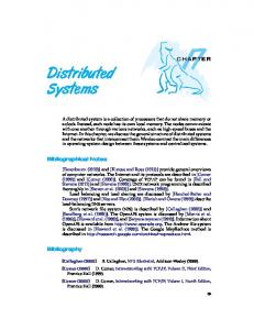
Once there were over 100 FCVs using the hydrogen fueling station, then the price trade-offs could go the other way: the price of on-peak electricity could be reduced in exchange for increased hydrogen prices. For example, with 200 FCVs utilizing the hydrogen from the 500-FCV station, hydrogen could be sold at $1.04/gallon equivalent to recover the fueling station equipment costs, which is near the current wholesale price of gasoline without taxes. The station owner could probably increase the price of hydrogen to something like $1.50/gallon, assuming that it would not be taxed initially to encourage clean fuels. In this case (hydrogen priced at $1.50/gallon with 200 FCVs), then the electricity could be sold at only 6¢/kWh for six hours onpeak, which might be a bargain for utilities faced with new T&D investments. Of course the owner may be in the enviable position of selling both electricity and hydrogen above their 10% return prices, making a greater return on investment. When the hydrogen fueling station was fully utilized (500 FCVs), the options become even more attractive. Hydrogen could be sold at $1.00/gallon, matching current wholesale gasoline with on-peak electricity sold to the grid at 6¢/kWh. In this case both state and federal highway taxes could be added to the hydrogen, as would be required in a mature FCV market. The previous figure assumed old natural gas commercial rates in California ($6.21/MBTU-HHV). The situation in Alaska would be much better, since natural gas has previously averaged only $2.37/MBTU3. As shown in Figure 2, peak electricity could be sold at 10.3¢/kWh, with hydrogen from a fully utilized fueling station (500 FCVs) sold at only $0.57/gallon equivalent. Even if only 100 FCVs were available, hydrogen could be sold at $1.50/gallon with on-peak electricity sold at 6.3¢/kWh.
3These natural gas prices are based on 1998 data. Well-head prices for natural gas have escalated sharply in 2001, from roughly $2/MBTU up to as much as $10/MBTU before dropping back to the $5 to $6/MBTU range in March of 2001. Many analysts expect that the recent resurgence of natural gas drilling will roll back some of these increases, but the commercial rates for natural gas will probably increase more than analysts projected just one year ago.
10
Electricity On-Peak Price (Cents/kWh)
20
Alaska Baseline: Natural Gas = $2.37/MBTU Electricity = 9.3 cents/kWh Designed for 500 FCVs 10,000 unit production volume 200-kWe Stationary Fuel Cell 6 hous of on-peak electricity sales
500 FCVs (Design Point) $0.57/gal
18
200 FCVs $0.72/gal
16
100 FCVs $1.09/gal
14
50 FCVs $1.82/gal
12 10 8 6
Electricity On-Peak Price for 10% ROI: 10.3 cent/kWh
4 2 0 0.50
0.75
1.00
1.25
1.50
1.75
2.00
2.25
2.50
Hydrogen Price ($/gallon of gasoline equivalent)
Figure 2. Estimated trade-offs in peak electricity and hydrogen prices in Alaska.
The previous two figures assumed that the utility bought back electricity during six hours of their peak load. Some utilities might be willing to pay more for peak electricity during a shorter period of time. Figure 3 illustrates the trade-off between electricity price and on-peak time for both California and Alaska. Thus a hydrogen fueling station owner in Alaska could make the goal of 10% return on investment by selling electricity at 10.3¢/kWh for six hours or for 20.6¢/kWh for three hours, etc.
Allowable Electricity Price (cents/kWh)
140
200-kW e Stationary Fuel Cell 10,000 Production Quantity Colocated at H2 Fueling Station
130 120 110 100 90 80 70 60
Alaska
50
(10.3 cents/kW h for 6 hours)
California (14.5 cents/kW h for 6 hours)
40 30 20 10 0 0
1
2
3
4
5
6
7
8
On-Peak Time (hours)
Figure 3. Allowable on-peak electricity price to make 10% real, after-tax return on investment as a function of the number of on-peak hours per day.
11
Electrolytic Hydrogen Assessment DTI also previously estimated the cost of hydrogen produced by electrolyzing water using off-peak electricity (Thomas-1998d, 1999c & 1999d). As shown in Figure 4, the cost of hydrogen generated by steam reforming of natural gas is competitive with taxed gasoline for large fueling stations supporting more than 1,000 FCVs (or 125 vehicles refueled per day.) However, the cost of trucking in liquid hydrogen gets prohibitive for stations supporting less than 1,000 FCVs. On-site reforming of natural gas is competitive for stations supporting more than 100 FCVs, assuming the development of factory-built, small-scale steam methane reformers (scaling down existing industrial SMRs would not be competitive.) In fact, hydrogen from these low cost, factory-built SMRs would be competitive with wholesale gasoline per mile driven.4 That is, a driver of a conventional vehicle would pay as much for wholesale gasoline (before road taxes) per mile as the driver of a hydrogen-powered FCV. 100
Electrolyzer (100 qty) Electrolyzer (1,000 qty) Electrolyzer (10,000 qty) Electrolyzer (100,000 qty) Electrolyzer (1 Million qty) BOC LH2 Praxair LH2 DTI/IFC SMR (1 qty) DTI/IFC SMR (100 qty) DTI/IFC SMR (1,000 qty) DTI/IFC SMR (10,000 qty) Gasoline ($3.86/gal - DM 1.84/liter) Gasoline ($1.5/gallon) Gasoline ($1/gallon) Air Products CH2 SMR Air Products LH2 Plant BOC On-Site SMR BOC LH2 Plant Praxair On-Site SMR Praxair LH2 Plant
On Site SMRs Trucked-In LH2
Hydrogen Cost ($/kg)
On Site Electrolyzers (4 cents/kWh)
Gasoline in Germany 10
US Taxed Gasoline @ $1.50/gallon
1 1
10
100
1,000
10,000
100,000
1,000,000
US Wholesale Gasoline @ $1.00/gallon
Number of Fuel Cell Vehicles Supported (Divide by 8 for number of vehicles fueled each day) Natural Gas Price for Regional SMRs
$4.74/GJ
Delivered Price of Trucked-In Liquid Hydrogen
Natural Gas Price for Trucked-In Hydrogen
$3.79/GJ
Capital Recovery Factor
$2.17/kg 0.1842
Natural Gas Price for On Site SMRs
$6.16/GJ
Electrolyzer Capacity Factor
0.7
Electrolysis Off-Peak Electricity Price
4.0 cents/kWh
On-Site SMR Capacity Factor
0.69
Electricity Price for SMRs
6.0 cents/kWh
LH2 Plant Capacity Factor
0.807
Electricity Price for LH2 Plants
5.0 cents/kWh
Fuel Cell Vehicle to Gasoline ICE fuel economy ratio (LHV)
2.2
(Gasoline price lines correspond to the cost of untaxed hydrogen to yield the same cost per mile driven in a fuel cell vehicle as in a gasoline-powered internal combustion engine vehicle) LH2 = Liquid Hydrogen; BOC = BOC Gases; DTI = Directed Technologies, Inc.; SMR = Steam Methane Reformer
DTI: H2-INFR.XLS; Tab 'LH2';AC176 - 5 / 15 / 2001
Figure 4. Estimated cost of 5,000 psi compressed hydrogen from various production sources, compared to the equivalent cost of gasoline on a per mile basis. 4The data in Figure 4 were updated from our previous reports to reflect increased cost of gasoline, natural gas and electricity.
12
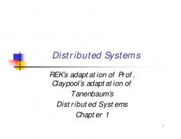
For fueling stations supporting fewer than 100 FCVs, however, even the on-site SMRs could not compete with wholesale gasoline. In the early days of FCV market penetration, many fleet owners would have fewer than 100 FCVs. For example, a company with 200 vehicles might only convert 5 or 10 vehicles to run on hydrogen initially to test out this new technology. In this case electrolyzers would provide the lowest cost hydrogen as shown on the left side of Figure 4, assuming that off-peak electricity could be purchased for 4 cents/kWh. Thus electrolyzers could provide lower cost hydrogen for small fleets or for public fueling stations during the early phases of FCV market penetration. However, electrolytic hydrogen has one major barrier in the United States: since over 55% of all U.S. electricity is generated from coal, using electrolytic hydrogen in a FCV in most parts of the U.S. would actually increase total greenhouse gas emissions compared to operating a conventional gasoline ICEV. Based on the average marginal U.S. grid generation mix, total greenhouse gas emissions would more than double for a FCV running on electrolytic hydrogen compared to the standard ICEV. As the electrical generation grid moves to increased use of renewable electricity and/or nuclear power, the FCV powered by electrolytic hydrogen will eventually be superior to even a FCV running on hydrogen from natural gas. In this task, we analyzed the necessary changes in the utility grid generation mix that would result in greenhouse gas parity for the FCV running on electrolytic hydrogen compared to an ICEV of the same size. The analysis of greenhouse gases from electrolysis should take into account the marginal utility generation mix. That is, adding a new electrical load such as a group of electrolyzers will require the electric utility to produce additional electricity. In general utilities run their lowest operating cost generators full time (if possible) as baseload. In general, this means turning on hydroelectric and any renewable energy first, followed by nuclear power, then coal, then natural gas, then oil and finally diesel fuel5. The marginal mix then depends on the time of day and the generation mix in a given region. Figure 5 illustrates the likely generation mix in Southern California before deregulation, based on the generators owned at that time by Southern California Edison and the Los Angeles Department of Water and Power. Between them, these LA utilities produced 36% of their electricity from natural gas, 32% from coal6, 22% from nuclear, and 10% from hydroelectricity. We have arbitrarily assumed that 40% of the natural gas is consumed in high efficiency (50% for air cooled and 54% for steam-cooled) combined cycle turbines, and 60% in single-cycle natural gas aeroderivative turbines at 35% efficiency for small units, to take into account the introduction of higher efficiency combined cycle turbines in the future. We added this distinction to illustrate that even as more combined cycle turbines are added, the older single-cycle turbines are moved to the top of the peak shaving list. As a result, adding new load such as an electrolyzer will necessarily mean more electricity from the older, less efficient plants during peak hours.
5This ranking from lowest cost to highest cost is based on operating costs only. On a life-cycle basis including capital recovery, natural gas turbines are less costly than coal-powered generators, while the coal costs less than natural gas per unit energy. Once the equipment is in place, however, the utilities tend to dispatch electricity on the basis of operating cost, not life cycle cost. 6Although there are no coal plants in California, these two utilities owned large coal plants in Utah and Nevada.
13
NG Turbine NG Combined Cycle Turbine
Coal
Nuclear Hydro & Renewables
0
12 Time (hours) 1
DTI: CFCP models.XLS; Tab 'GHG';J53 - 5 / 10 / 2001
Hydro
Increasing Marginal Cost
Generation Mix
Hypothetical Load Profiles 1 0.9 0.8 0.7 0.6 0.5 0.4 0.3 0.2 0.1 0
Nuclear
Coal
NG Combined Cycle
24 NG Turbine
Figure 5. Illustration of likely marginal electronic grid generation mix in the Los Angeles area.
Returning to Figure 5, the two daily load lines illustrate the likely marginal grid mix for electrolyzers (and other new loads) – adding new loads will draw power from the generators just above the load profile at any time of the day. As new loads come on line, the utilities will increase output from the marginal (highest operating cost) generators. With the top load profile in Figure 5, this would imply that all electrolyzer electricity should be attributed to a mix of low efficiency and higher efficiency gas combined cycle turbines. No credit is given for either nuclear, hydroelectric or particularly renewable electricity, which is all baseload, operated 24 hours per day whenever possible. The lower load profile in Figure 5 is even worse. With this profile, the utilities would have to turn on coal generators at night to supply electrolyzers added to the grid. Thus off-peak electricity might be less expensive, but in this case it would produce considerably more greenhouse gases due to the increase in coal generator output. Advocates of using electrolyzers to produce hydrogen have suggested that new renewable energy such as from wind turbines could be used to reduce greenhouse gases. In this concept, electricity from remote wind turbines would be wheeled to the local fueling station over the utility grid. These green electrons would then be converted to hydrogen for FCVs, which would then reduce GHGs by displacing gasoline-powered ICEVs. From a societal viewpoint, however, this may not be optimum utilization for these green wind electrons. Another option is simply to displace electricity produced from existing electrical generators, thereby also reducing greenhouse gas emissions. As shown in Figure 5 above, displacing grid electricity even in California which has a high fraction of nuclear and hydroelectric power would cut down GHGs by reducing fuel burned in natural gas or even coal turbines. In fact, displacing grid electricity does reduce GHGs more than making hydrogen for FCVs as shown in Figure 6. Depending on the marginal grid mix, displacing grid electricity with wind power in the LA basin would reduce GHGs by about 600 to 800 grams of CO2-equivalent for each kWh of wind electricity. This same kWh of wind electricity would produce enough electrolytic hydrogen to cut GHGs by only 300 to 500 grams of CO2, depending on the type of electrolyzer and the fuel economy of the FCV relative to a gasoline ICEV. We show two types of electrolyzers in Figure 6: a conventional electrolyzer with atmospheric pressure hydrogen output, and an electrolyzer with 300 psia hydrogen output. The higher pressure electrolyzer reduces the compressor load, thereby using less electricity to compress the hydrogen to 7,000 psi for storage. We also show two fuel economy ratios: 1.7 to one and 2.2 to one. The 2.2
14
fuel economy improvement corresponds to our estimate for a mature FCV. Early FCVs will probably be less efficient, which would reduce the GHG savings from electrolytic hydrogen. Electrolyzer (300 psia @ 1.7 f.e. ratio) Electrolyzer (1 atm @ 1.7 f.e. ratio)
Gasoline Displacement by H2 FCV
Electrolyzer (300 psia @ 2.2 f.e. ratio) Electrolyzer (1 atm @ 2.2 f.e. ratio)
NG CC (steam-cooled turbine) NG CC (air-cooled turbine)
Grid Electricity Displacement
50% NG/ 50% NGCC Small NG turbine (35.4% eff) 50% NG/ 25% NGCC/ 25% Coal Coal at 34% efficiency f.e. = fuel economy ratio (FCV/ICEV)
-
200
400
600
800
1,000
1,200
1,400
Greenhouse Gas Reductions (grams of CO2-equivalent/kWh) Large Reductions are Good
DTI: CFCP models.XLS; Tab 'GHG';K87 - 5 / 10 / 2001
Figure 6. Illustration of greenhouse gas reductions, comparing the use of electrolytic hydrogen in FCVs to displace gasoline in ICEVs (upper four bars), with displacing grid (lower six bars).
Some proponents of electrolyzers have suggested that the grid could not accept wind power at night. If this were the case, then making hydrogen for use in FCVs would be a net reduction in GHGs. However, once a wind turbine is installed, a utility operator will always operate it 24 hours per day (or at least whenever the wind is blowing) as baseload, since it has the lowest operating costs. The operator will therefore turn down virtually any other generator at night to accept the low cost wind energy to minimize overall costs. Therefore wind power will not be rejected until such time that the grid has more wind electricity at night than the night time load. The key question for wind/electrolysis/hydrogen systems is when will wind power grow to equal the minimum utility off-peak load? Projecting future utility grid mix is difficult, but we can make some general observations: 1. Current coal-based plants which produce over 50% of all U.S. electricity today are under-utilized, despite the fact that they can generate electricity at costs between 1 to 3¢/kWh, less than the cost of electricity produced by a new combined cycle gas turbine system. U.S. coal plant utilization has been averaging around 62%. Thus increased demand caused by electrolyzers could increase coal electricity production, the worst outcome from a GHG perspective. 2. Nuclear power generation was not expected to grow and may even have decreased over the next few decades as plants are retired and not replaced, again placing pressure to use more coal-based electricity. The new Bush administration will attempt to revive the nuclear power industry, but under the best political circumstances no new nuclear plants are likely for at least 15 years. Any reduction in nuclear power production would shift the marginal electricity mix toward more coal during off-peak hours where nuclear power may have dominated previously. 3. Most new generation capacity will be based on very efficient combined cycle gas turbines running on natural gas. Efficiencies up to 48% are feasible today, with projections as high as 54% forecast by some
15
observers. Gas turbines can also be cycled up and down in power quickly, making them the logical choice to handle peak power loads. 4. Even the most optimistic projections of renewable energy grid penetration do not show significant contributions over the next few decades. Figure 7 illustrates the electrical generation mix that would be required to reduce greenhouse gases for hydrogen produced by electrolysis. The upper horizontal line indicates that the ICEV would produce about 415 grams/mile of CO2-equivalent emissions. The lower horizontal line shows that hydrogen produced from natural gas would reduce GHGs by about 40%. The sloped lines project the GHGs for a direct hydrogen FCV running on electrolytic hydrogen from the power grid as function of the fraction of the marginal grid mix consisting of some combination of nuclear and renewables. If we start with the current average grid mix in the U.S. (not the marginal mix), then the fraction of renewables and nuclear would have to increase to about 60% before the FCV greenhouse gas emissions would be reduced to the level of the gasoline ICEV, and to about 74% renewables and nuclear to match the current greenhouse gas emissions of a FCV using natural gas-derived hydrogen. 900 Fuel Cell Vehicle on Electrolytic Hydrogen @ 66 mpgge Starting with Current Grid Mix
800
Greenhouse Gas Emissions (g/mile of CO2-equivalent)
700
Fuel Cell Vehicle on Electrolytic Hydrogen @ 66 mpgge Assuming Natural Gas Combined Cycle @ 45% Efficiency
600 Conventional Car (ICEV) on gasoline @ 30 mpg
500
400 Fuel Cell Vehicle on Hydrogen from Natural Gas @ 66 mpgge 300
200
100
NGCC with 54% Efficiency 0 0.3
0.4
0.5
0.6
0.7
Fraction of Renewables & Nuclear
0.8
0.9
1
DTI: GHG.X LS, A A231;5/10/2001
Figure 7. Greenhouse gas emmissions from FCVs powered by electrolytic hydrogen, compared to ICEVs (upper horizontal line) and FCVs with hydrogen from natural gas (lower horizontal line)
The two lower sloped lines in Figure 7 correspond to the GHG emissions assuming that all marginal grid electricity came from natural gas combined cycle plants, operating at 45% efficiency (current technology) to 54% efficiency (projected potential with steam-cooled combined cycle natural gas turbines). In this case, renewables and nuclear would need to account for 50% of marginal power to 40% in the case of the 54% efficient combined cycle plants. From this analysis, we need to achieve more than 70% renewables plus
16
nuclear grid penetration with the existing grid, or some combination of large-scale introduction of natural gas combined cycle plants in conjunction with 40% to 50% renewables plus nuclear. What is the likelihood of either combination? The standard energy forecasts by groups like the U.S. Department of Energy’s Energy Information Administration do not forecast any significant growth in renewables and nuclear by 2020, the end of their time horizon as illustrated in Table 3. We have also included some forecasts by other groups including the Gas Research Institute, Standard & Poor’s DRI and the WEFA. None of these forecasts show renewables and nuclear above 23% penetration by 2020. Table 3. Projections of the average U.S. grid mix for 2015 and 2020. Coal
Oil
NG
Nuclear
Renewables (Hydro)
Sum of Renewables & Nuclear
2015 - AEO Reference Case 2015 - AEO Low Economic Growth 2015 - AEO High Economic Growth 2015 - WEFA Group 2015 - Gas Research Institute 2015 - Standard & Poor's DRI
52.1% 52.5% 52.4% 39.6% 56.3% 47.6%
1.0% 0.8% 1.3% 0.6% 0.7% 2.8%
25.7% 24.5% 26.0% 41.1% 24.1% 26.9%
12.1% 12.6% 11.5% 8.2% 9.9% 12.9%
9.1% 9.6% 8.7% 10.5% 8.9% 9.8%
21.2% 22.2% 20.2% 18.7% 18.9% 22.7%
2020 - AEO Reference Case 2020 - AEO Low Economic Growth 2020 - AEO High Economic Growth 2020 - WEFA Group 2020 - Standard & Poor's DRI
52.1% 52.4% 54.6% 38.8% 46.1%
0.8% 0.7% 1.3% 0.5% 2.9%
28.5% 27.1% 26.5% 43.5% 30.3%
9.7% 10.4% 9.3% 6.1% 11.5%
8.9% 9.5% 8.4% 11.1% 9.2%
18.6% 19.8% 17.7% 17.2% 20.7%
Annual Energy Outlook 2000
One of the most optimistic projections for renewable energy was made by a group of environmental organizations7 in 1990. They published a report entitled “America’s Energy Choices,” outlining several scenarios. The most optimistic of these scenarios was their “climate stabilization” plan, which predicted the generation of 1,500 terawatthours of electricity from renewables by 2030, which would amount to 61% of all electricity generated in that year (this scenario also assumes a 50% reduction in electricity consumption, requiring far greater energy efficiency improvements than any other projection). However, actual renewables have fallen well below the American’s Energy Choices pathway in the ten years since it was published, as shown in Figure 8. In fact, actual introduction of renewables has been negligible on a national scale compared to total grid energy production. The actual renewable energy (98% hydroelectric) has in fact fallen below the AEC “reference case,” the least optimistic projection for renewables, and is less than half the projected level for the climate stabilization scenario. At the very least, we have lost a decade in pursuing the aggressive climate stabilization pathway, and there is very little to indicate that the U.S. will embark on this pathway anytime soon.
7The AEC group included the Alliance to Save Energy, the American Council for an Energy-Efficient Economy, the Natural Resources Defense Council and the Union of Concerned Scientists.
17
1,600 1,400
Renewable Electricity (terawatt hours/year)
AEC = America's Energy Choices Actual Renewables is 98% hydroelectric
1,200 1,000 800 600 AEC Climate Stabilization
400
AEC Environmental AEC Reference
200
Actual Renewables
1990
2000
2010
2020
2030
Year DTI GHG XLS AB163 9/21/2000
Figure 8. Comparison of the AEC 1990 projections for renewable energy growth with the actual renewable electricity over the last decade.
We also looked at several longer range projections to the year 2050 by two organizations: the World Energy Council (WEC) and the Electric Power Research Institute (EPRI). As shown in Figure 9, only the most optimistic of these scenarios would yield a significant reduction in GHGs from direct hydrogen FCVs using electrolytic hydrogen by the year 2050. And none of these pathways would provide lower GHGs than a FCV using hydrogen from natural gas today. However, this figure is based on the average utility grid mix projected for 2050, not the marginal grid mix. Depending on the circumstances at that time, the marginal grid mix could produce lower GHG emissions.
18
FCV @ 66 mpgge & H2 from natural gas ICEV @ 30 mpg:
All FCVs using Electrolytic Hydrogen from Projected 2050 Average US Grid Mix: EPRI High Renewable & Nuclear EPRI Technology Roadmap High Coal WEC Ecologically driven, nuclear renaissance WEC Ecologically driven WEC Moderate Growth WEC High growth, transition to post-fossil fuel WEC High growth, coal emphasis WEC High growth, plentiful oil FCV = Fuel Cell Vehicle; ICEV = Internal combustion engine vehicle; EPRI = Electric Power Research Institute WEC = World Energy Council (1998)
0
100
200
300
400
500
600
Greenhouse Gas Emissions (g/mile)
Figure 9. Estimated greenhouse gas emmissions from a FVC using electrolytic hydrogen produced from the projected average utility grid mix in 2050, compared to gasoline ICEVs and FCVs powered by hydrogen made from natural gas.
We conclude that electrolytic hydrogen in the U.S. is unlikely to reduce greenhouse gas emissions when consumed by a FCV for at least three decades, and possibly longer, unless the country begins to aggressively invest in renewable energy or nuclear energy. There may also be some regions of the nation such as the Pacific Northwest where the grid is sufficiently “green” to produce a net reduction of greenhouse gases. In addition, off-grid applications such as a wind or PV system connected directly to an electrolyzer would essentially eliminate any greenhouse gas emissions. The situation is not much better in most parts of the industrialized world. Most of central Europe uses considerable coal in their electrical generation mix. The five major nations with electrical generation capacity favorable to electrolysis are Brazil, Canada, France, Norway and Sweden, as shown in Table 4 below. All other major nations of the world would produce more greenhouse gases with electrolysis than by burning gasoline in current vehicles.
19
Table 4. Electricity grid mix (percentage) for major nations (consuming over 100 billion kWh) in 1997
Electricity Production (Billion kWh)
Hydro
Coal
Oil
Gas
Nuclear
Australia
182.6
9.2
80.1
1.3
7.6
-
Brazil
307.3
90.8
1.8
3.2
0.4
1.0
Canada
575
61.1
17.4
2.4
4.1
14.4
China
1,163.4
16.8
74.2
7.2
0.6
1.2
France
498.9
12.5
5.2
1.5
1.0
79.3
India
463
16.1
73.1
2.6
6
2.2
Italy
246
16.9
10
46
24.9
-
Japan
1,029
8.7
19.1
18.2
20.5
31
Korea
244
1.2
37.4
16.8
13
31.6
Mexico
175
15.1
10
54.3
11.5
6
Norway
110
99.4
0.2
-
0.2
-
Poland
141
1.4
96.7
1.4
0.2
-
Russia
833
18.8
16.8
5.3
45.3
13.1
Saudi Arabia
104
-
-
57.5
42.5
-
South Africa
208
1
92.9
-
-
6.1
Spain
186
18.6
34.3
7.2
8.8
29.8
Sweden
149
46.2
1.9
2.1
0.5
46.8
Turkey
103
38.5
32.8
6.9
21.4
-
Ukraine
178
5.5
27.6
4.3
17.9
44.7
UK
344
1.2
34.8
2.3
31.3
28.5
US
3,670
9
53.8
2.9
13.8
18.2
20
Hydrogen Produced from Methanol On-Site8 We explored the economics of using methanol as the hydrogen carrier from remote low-cost natural gas sources to the fueling station9. That is, methanol would be reformed at the local fueling station to provide hydrogen for a direct hydrogen FCV. The intent of this option would be to exploit the low cost stranded natural gas from remote sites including sea-based oil platforms. The natural gas that was previously flared for lack of a market would be converted to methanol, shipped by tanker ship to the major nations, and then to the local fueling station where it would be converted to hydrogen for storage on the FCV. We explored two aspects of the methanol route: the cost of the stationary methanol reformer, and the likelihood of oil and gas companies converting stranded natural gas to methanol instead of the other options for monetizing remote natural gas. This particular option might also have benefits should automobile manufacturers build both methanol and hydrogen-powered FCVs. Capital Cost Estimates for Small-Scale Stationary Methanol Fuel Processors The chemical conversion of methanol to hydrogen-rich gas mixtures has been studied intensively since the petroleum crisis of the 1970’s. Two principal pathways have traditionally been evaluated, steam reforming (SR) of methanol with water and autothermal reforming (ATR) of methanol with air and water. The former has been demonstrated widely, and has well-known operating parameters over the preferred catalysts, mixed oxides of copper and zinc stabilized by alumina. The latter pathway has been demonstrated at Argonne National Laboratory and by Johnson Matthey PLC in Great Britain. These efforts in autothermal reforming have been conducted more recently, and less is known about catalyst durability, a central problem with the copper-based catalysts used in methanol systems, especially at the high temperatures characteristic of autothermal reforming. Whether the conversion is accomplished through SR or ATR, methanol conversion requires a less sophisticated chemical process train operating at lower temperatures than competing hydrogen production techniques based upon other fuels such as natural gas. Lower temperature methanol reformers should have lower capital cost compared to natural gas, naphtha, or gasoline reformers. This study compares the likely manufacturing cost of SR and ATR reformers based on traditional catalyst compositions in combination with commercially available pressure swing adsorption (PSA) gas cleanup equipment. The reformers are sized such that a packaged system could support a 50-vehicle fleet. Assuming that each vehicle travels 12,000 miles per year, each vehicle would require on average 0.5 kg of hydrogen fuel per day10. If a capacity factor of 69% is assumed to cover daily and seasonal demand variation, the 50-car station would produce at least 36 kg/day at peak capacity. In previous research conducted by the authors (Thomas-1997a), a small-scale reformer system for natural gas included six reforming modules with a capacity of 8 kg/day each. 8Frank Lomax is the primary author of this section 9This task was suggested by Dave Nahmias, at the time Chairman of the DOE Hydrogen Technical Advisory Panel (HTAP). 10This hydrogen consumption assumes a 5-passenger vehicle such as a Ford AIV (aluminum intensive vehicle) operating on a 1.25 times accelerated EPA combined cycle (45% highway and 55% city driving). We estimate a fuel economy of 66 mpgge on this accelerated driving schedule.
21
This represented a capacity factor of just over 50%, but allowed one entire unit to be removed for service without interrupting operation of the refueling station. Further, the manufacture of identical subassemblies allows higher volume manufacturing techniques than would otherwise be appropriate. In this study, it is assumed that reformers are manufactured to serve 500,000 vehicles that are assumed to be sold over a six-year period. It is assumed that the vehicles are sold at the rate of 83,000 units per year, and that a total of 10,000 50-car refueling stations are required over that same period. For reformers employing six identical subassemblies, 10,000 subassemblies would be produced each year. The general configuration of the refueling station is shown in Figure 10. The reformer subassemblies produce hydrogen-rich reformate gas at elevated pressure (7 bar – 20 bar). This gas is cooled in an intercooler, condensate is removed in a liquid trap, and the dry, cool gas is delivered to the PSA unit. Here, the impurities are adsorbed onto a high surface area adsorbent, and the clean hydrogen passes through the bed with a nominal pressure loss (< 1 bar). Periodically the pressure on the bed is then reduced, and the impurities are desorbed and returned to the system for subsequent combustion to provide energy to the process. The clean, pressurized hydrogen is then delivered to the compression and storage subsystems for greater pressurization, storage and subsequent delivery to the vehicles during refueling. The hydrogen compressor and storage tank costs were considered in previous research by the authors, and will be used again in this study. The PSA unit assumed here is based on the HyQuestorTM 605 that is manufactured by QuestAir Technologies11. Also included in the refueling system is an electronic controller and a compressed nitrogen supply system for valve operation and safety purging12. It is assumed here that the reformers are operated continuously at some level in order to maintain the catalyst in the reduced state. If intermittent operation is desired, a hydrogen supply system and feed valves will be required to reduce the catalyst.
11 QuestAir Technologies was formerly named Questor Industries, Inc. 12 The nitrogen employed will require an oxygen content of about 100 ppm for shutdown purposes, as the reduced copper catalysts are pyrophoric, and must be gradually returned to their stable, oxidized state upon shutdown.
22
MeOH storage
Reformer Subsystem
PSA Subsystem
Compression Subsystem
H2 Storage Subsystem
Dispensing Subsystem
Control Subsystem N2 Subsystem H2 (optional) Subsystem
Utilities
Figure 10. Methanol-based Hydrogen Fueling Station Process Flow
Because the SR and ATR MeOH reformer subsystems are fundamentally different in their design, they will be addressed separately in the following paragraphs. The balance of the refueling system is essentially identical for the two technologies, and is based on previous research conducted by the authors that will be briefly summarized after the detailed discussion of the reformer subsystems. Methanol Steam Reformer Subsystem Methanol steam reforming is typically carried out over a “mixed oxide” catalyst containing oxides of copper, zinc and aluminum. The formulation and mechanical form of these catalysts are typically similar to those for water gas shift reactors in high temperature fuel reformer systems such as those employed for the reformation of natural gas or naphtha. Operation in the steam reforming mode on such catalysts is limited at low temperature by the formation of condensate on the catalysts at the dew point for the pressure of operation, and on the high side by sintering of the catalyst, which becomes appreciable above 260°C (Pepley-1997). Because the methanol reforming reaction is endothermic, heat transfer must be accomplished between a hightemperature gas stream and the cooler reactants. The hot gas is typically produced by combustion of unused hydrogen, carbon monoxide and methanol in the tailgas from the PSA purification system, with oxygen from air. The adiabatic flame temperature of this gas is typically well above the 260°C temperature limit for the mixed oxide catalysts. Further, heat transfer between the gas and the reforming catalyst is difficult to achieve. For these reasons, a number of groups have demonstrated methanol steam reformers that utilize an intermediate heat transfer fluid such as a high-
23
temperature oil that is heated in a separate heat exchanger by the combustion gas and then passed over tubes containing the reforming catalyst and the reacting steam-methanol mixture. Thus, a methanol steam reformer system usually comprises the following: • • • • • • • • •
a heat exchange reactor that allows for rapid heat exchange between a heat transfer fluid and the catalyst zone where reaction occurs a separate heat exchanger for heating the heat transfer fluid with hot gases a combustor for burning the fuel gas in air prior to heating the heat transfer fluid. a vaporizer where the fuel/water mixture is boiled and superheated to the reactor inlet temperature an intercooler where the hot reformate gas can be cooled by the incoming combustor air before being sent to the PSA unit a condensate trap for removing condensed water and methanol an air blower to provide combustion/cooling air a water deionization system feed and recirculation pumps for the various feedstocks
Additionally, the system requires control thermocouples, pressure relief devices, and appropriate valves to control the process flows. A system of this type is illustrated in Figure 11. Valves and sensors are omitted from this diagram. This proposed system is a hybrid of the high temperature, adiabatic methanol steam reformer patented by Engelhard (Beshty-1990) and the essentially isothermal reformers used by other workers13.
13 The isothermal approach seems to have been first patented by Hidetake Okada of Nippon sanso Kabshiki Kaisha in Tokyo, Japan. This patent # 4,865,624 is dated Sep. 12, 1989. This design has subsequently been used by Amphlett, et al of the Royal Military College of Canada and Daimler Benz Ballard (dbb) in their NECAR 3 system.
24
exhaust Oil circulation pump
Oil-Air HX MeOH HX reactor
MeOH Feed Boiler
DI
Air blower
water cartridge combustor
Water Reformate-Air HX
Condensate trap
Separated tailgas from PSA Condensate recycled to inlet as feed
Product reformateto PSA
Figure 11. Methanol Steam Reformer System Schematic
Excellent research by Amphlett and Pepley, et al (1997) has provided kinetic data for such oil-heated methanol steam reformers. Extrapolation from their data suggests that a methanol steam reformer based on mixed oxide catalysts and operated in a high pressure regime suitable for use with a PSA system (15 – 20 bar) would require roughly 0.2 kg of catalyst per kW thermal of hydrogen produced. This is based upon a reformer utilizing 12.7 mm o.d. reformer tubes. Their data suggest heat transfer limitations, which may make a reactor based upon smaller tubes even more compact. If each subassembly is designed to produce 8 kg of hydrogen per day, and the PSA system recovers 80% of the hydrogen produced (McLean-1997), then each subassembly will require approximately 2.75 kg of catalyst if 12.7 mm reformer tubes are used. Whereas the industrial catalysts typically used in research are nominally 3mm right cylindrical extrudate with a specific gravity of about 1.35, it is assumed here that a finer extrudate is used in the small-scale reformers to facilitate rapid heat transfer, good flow distribution, and easy reactor loading. The specific gravity of such a catalyst is assumed to be approximately 2. No improvements in kinetics are expected, as reactor testing has confirmed that the industrial catalysts have a high effectiveness factor (Amphlett-1988). Table 5 illustrates the amount of tubing of each size required for each subassembly. These calculations assume that a spiral tube-in-tube geometry is employed. This type of construction requires a minimal number of seals, all of which can be readily and inexpensively accomplished through either manual or automatic gas
25
tungsten arc welding (GTAW). Spiral tube heat exchangers are often employed in the chemical process industry, but are not usually considered for mobile applications because they are ill suited for operating environments involving mechanical shock as the tubing is not well-supported. In the proposed design, the inner reformer tubes are first inserted into a larger diameter outer tube then the assembly is bent using an automatic tube-bending machine. For the purposes of this study a 3-pass design using 12.7 mm o.d. tubes as the reformer tubes and 38 mm o.d. tubing for the outer tube is assumed. In this configuration, tubing would have to be shipped in 5 m (~15’) lengths, which is feasible. The coiled tubing can then be supported in a protective housing formed from 20 cm o.d. tubing. The tubes are supported on stamped frames that support each loop at four points. The supports can be attached to the tube bundle, then riveted to the protective housing. Insulation can also be provided between the tube bundle and the housing wall to minimize heat losses. It is assumed that ceramic felt insulation is employed for that purpose. Figure 12 shows a schematic view of the completed spiral heat exchange methanol steam reformer. Table 5: Tube geometry for methanol steam reformers Tube geometry 10 mm (0.375") 12.7 mm (0.5") volume per length (cc/m) 47 94 catalyst mass per length (g/m) 94 187 total length required for subassembly 21.2 14.7 # of 15 cm diameter loops required, 1 pass 45 31 # of 15 cm diameter loops required, 2 pass 23 16 # of 15 cm diameter loops required, 3 pass 15 10
Feedstock inlet Hot oil inlet
Protective housing
Reformer tubes Insulation
Hot oil outlet Reformate outlet
Figure 12. Spiral Methanol Steam Reformer Schematic
Construction of a large number of compact heat exchangers could present a manufacturing cost obstacle, especially if each unit required separate tooling, materials of construction, etc. For the purposes of this study, it is assumed that brazed plate-fin heat exchangers with identical plate dimensions are used for all of the system heat exchangers. The capacity of the individual units is then adjusted by increasing or decreasing the number of plates used. It is assumed that 25 cm by 10 cm plates are used with each “plate” including a 0.5 mm separator plate, a 2.4 mm thick manifolding frame, and a stamped finsheet 23 cm x 7.6 cm by 2.4 mm
26
high. The heat exchanger fins are assumed to be spaced 22 fins per inch and stamped from 0.1 mm (0.004”) thick stainless steel foil14. We assume that 409 stainless steel is used, and that the separator plates are clad with nickel brazing alloy. This type of construction has been demonstrated industrially for maximum temperatures up to 550°C. The stamped components are assembled and brazed in a continuous hydrogen belt furnace. The combustor uses a combustion catalyst to burn the tailgas from the PSA unit to provide process heat for the reformer system and to reduce emissions of pollutants such as carbon monoxide. The combustor is also used during startup to bring the reformer components up to temperature, and must thus have a preheater and a means of delivering unreacted liquid methanol. The combustor comprises the following: • • • • •
a catalyzed monolith loaded with a combustion catalyst such as Pd-Pt on -alumina a sheet metal housing that contains the catalyst and allows mounting to the structural frame a refractory liner to protect the housing and fuel injection system from temperature excursions a low pressure fuel injector to deliver atomized liquid methanol an electric heating element (automotive glowplug) to bring the combustion catalyst to light-off temperature during startup
The methanol steam reformer requires 18 feed and circulation pumps that deliver reactants, recycle condensate, circulate heating oil, and deliver neat methanol for startup. The oil is circulated with a gear pump, since this type of pump is well-suited to handling high-temperature fluids at moderate pressure head. A gear pump with a fixed-speed, 110 VAC drive is assumed. For recycling condensate and metering methanol and water at high pressure, OEM-style metering pumps like those supplied by FMI are assumed. These pumps will allow a nominal delivery pressure of 10 bar. It is assumed that both the methanol and water feed pumps are driven by a single variable speed 110 VAC drive, as their delivery ratios are fixed. The condensate pump is driven by a fixed-speed 110 VAC drive that is controlled by a float switch. The condensate trap is a simple stainless steel vessel with a float switch. The system also requires a variety of valves, relief devices and temperature probes. A back-pressure regulator is employed to control delivery of reformate product to the PSA system. A zero back-flow regulator will also act as a check valve to protect the reformer system from over-pressure should a failure occur in the downstream processes. A nitrogen purge solenoid valve is required for safety reasons should an overtemperature or over-pressure situation occur. A hydrogen delivery solenoid valve is also required for system startup. A minimum of two pressure relief valves are required, one for the reactant loop and one for the pressurized heat transfer fluid. For full code compliance, a relief device of some kind must be provided on each high pressure device or one device each for the evaporator, oil heater, reactor, and intercooler. All four of the relief valves can be reseating valves with high-temperature seals such as Kalrez. A minimum of five control thermocouples are necessary: in the combustor, after the combustor, in the air stream after the evaporator, in the hot oil loop after the oil heater, and in the reformate outlet. It is assumed that an automotive ECU-type controller is supplied for each subassembly, and that this controller interacts with the refueling 14 Fins of this type can be produced using machinery provided by Robinson Fin Machines, Inc. that is capable of stamping 300 fins per minute, or ~35 cm of 23 cm wide fin material per minute.
27
station control system. The manufacturing cost of the system is estimated based upon the Design For Manufacture and Assembly (DFMA)15 techniques pioneered by Boothroyd and Dewhurst and used previously by the authors to estimate manufacturing costs for various systems. The estimated cost and bill of materials for the steam reformer system is shown in Table 6. Surprisingly, this cost is higher than that previously estimated by the authors for a steam methane reformer subassembly that operates at much higher temperature. Analysis of the estimates shows that a significant cost is incurred as a result of pumps for each subassembly, over $500. This suggests that one pathway to reduce cost would be to implement a centralized pumping concept as applied to the steam methane reformer. Also, the fact that this system is configured to operate with a PSA system instead of a high-temperature metallic membrane leads to the requirement for intercooling, condensate recovery, and condensate recycle. All of this suggests that the totally modular approach that proved appropriate for steam methane reforming using a high-temperature metal membrane may not be appropriate for a steam methanol reforming system.
15DFMA is a registered trademark of Boothroyd Dewhurst, Inc.
28
Table 6. Budgetary estimate of the steam methanol reformer subassembly assembly name
component name
finished part dimensions (cm) L W (od) D (id or t)
part characteristics mass volum materi part (kg) e (L) al cost materi ($/kg al cost
mfg. Cost
7.9
1.317
0.167
$6.60
$0.50
$9.19
$13.22
$39.65
7.9
4.571
0.579
$6.60 ##### $0.50
$30.67
$44.08
$44.08
7.9
0.448
0.057
$3.30
$5.00
$6.48
$8.10
$16.19
7.9
2.814
0.356
$6.60 ##### $1.00
$19.57
$24.46
$24.46
0.1
7.9
0.496
0.063
$6.60
$3.27
$1.00
$4.27
$6.14
$12.29
6
0.1
7.9
0.27
0.034
$6.60
$1.78
$0.25
$2.03
$2.92
$11.69
20
16
0.5
3.222
6.443$10.76/sqm$3.85
$0.02
$3.87
$4.84
$4.84
2.75
1.375 ##### #####
$37.13
$46.41
$46.41
usage
make/buy
material
reformer tube
3
buy
316L
500
1.27
1.09
heat exchange jacket
1
buy
316L
498
3.8
3.6
end boss fitting
2
make
316L
5
3.8
0
outer housing
1
make
316L
57
20
19.8
end dome
2
buy
316L
5
20
tube support
4
buy
316L
57
insulation blanket
1
make
ceram fiber
57
catalyst
1
make
G66B
s.g.
Total unit cost before
markedup unit cost
total cost w/ markups
assem bly mfg.
steam reformer $8.69 $1.48
##### evaporator assembly separator plate
11
buy
409
25
10
0.05
7.8
0.099
0.013
$2.00
$0.20
$0.27
$0.47
$0.67
fin sheet
11
buy
409
23
23.4
0.01
7.8
0.043
0.005
$4.00
$0.17
$0.10
$0.27
$0.39
$7.39 $4.27
manifold frame
11
make
409
25
10
0.24
7.8
0.474
0.06
$1.50
$0.71
$0.10
$0.81
$1.01
$11.15
end plate
2
make
409
25
10
0.24
7.8
0.474
0.06
$1.50
$0.71
$0.10
$0.81
$1.01
$2.03 $6.25
oil heater assembly separator plate
11
buy
409
25
10
0.05
7.8
0.099
0.013
$2.00
$0.20
$0.27
$0.47
$0.67
fin sheet
11
buy
409
23
23.4
0.01
7.8
0.043
0.005
$4.00
$0.17
$0.10
$0.27
$0.39
$7.39 $4.27
manifold frame
11
make
409
25
10
0.24
7.8
0.474
0.06
$1.50
$0.71
$0.10
$0.81
$1.01
$11.15
end plate
2
make
409
25
10
0.24
7.8
0.474
0.06
$1.50
$0.71
$0.10
$0.81
$1.01
$2.03 $6.25
intercooler assembly separator plate
21
buy
409
25
10
0.05
7.8
0.099
0.013
$2.00
$0.20
$0.27
$0.47
$0.67
fin sheet
21
buy
409
23
23.4
0.01
7.8
0.043
0.005
$4.00
$0.17
$0.10
$0.27
$0.39
$14.11 $8.15
manifold frame
21
make
409
25
10
0.24
7.8
0.474
0.06
$1.50
$0.71
$0.10
$0.81
$1.01
$21.29
end plate
2
make
409
25
10
0.24
7.8
0.474
0.06
$1.50
$0.71
$0.10
$0.81
$1.01
$2.03 $8.75
combustor assembly bottom housing
1
make
316L
30
10.16
10
7.9
0.6
0.076
$6.60
$3.96
$1.00
$4.96
$6.20
$6.20
top housing
1
make
316L
20
10.16
10
7.9
0.4
0.051
$6.60
$2.64
$1.00
$3.64
$4.55
$4.55
refractory liner
1
make
fiberfrax
40
10
7.5
1
1.374
1.374
$3.00
$4.12
$1.00
Pt-Pd on ZTM
1
buy
20
7.5
0
0.974
0.86
0.883 $81/L #####
glowplug
1
low pressure fuel injector
1
$5.12
$6.40
$6.40
$71.53
$89.42
$89.42
buy
$10.00
$14.38
$14.38
buy
$5.00
$7.19
$7.19 #####
pumps, valves and misc. condensate pump and drive
1
buy
$50.00
$71.88
condensate trap and float
1
buy
$50.00
$71.88
$71.88 $71.88
MeOH & water pump
2
buy
$35.00
$50.31
$100.63
variable speed motor
1
buy
$100.00
$143.75
$143.75
gear pump and drive
1
buy
$75.00
$107.81
$107.81
ASME relief valve
4
buy
$5.00
$7.19
$28.75
backpressure regulator
1
buy
$20.00
$28.75
$28.75
gas feed solenoid
2
buy
$20.00
$28.75
$57.50
k-type thermocouple
5
buy
$5.00
$7.19
$35.94
ECU
1
buy
$240.00
$345.00
$345.00
subtotal
$1,415
plumbing allowance
$100.00
total
#####
$1,567.39
If the system were modified to a slightly more conventional layout where the combustor, intercooler, oil heater, and vaporizer functions were centralized, several advantages might acrue. First, the number of feed pumps required would be reduced to three per refueling station instead of eighteen. The number of combustor units would be reduced to one from six, and the number of oil feed pumps would be similarly reduced. The reactors, which are readily manufactured using high-volume techniques, would remain modular, and they could either be operated as independent loops through the use of on-off valves in the reactant and coolant loops, or they could be operated at varying space velocity. The provision of valves would be more desirable as it would better facilitate removal of individual units for repair. The economies of scale lost in the heat exchanger production would be essentially negligible, as the unit elements of the heat exchangers would
29
remain identical, and be produced in similar volumes. The units would likely be batch brazed at higher cost, but the difference is likely to be rather small as the batch furnace would be run semi-continuously as roughly 25 large heat exchangers would have to be produced per working day. This may require two furnaces or more as the cycle times for such components can be several hours. The impact on the cost of the pumps and valves is more difficult to assess, as these components then become essentially low-production, bought components, for which overhead charges become much more substantial. A detailed analysis of the cost of a more traditional system is beyond the scope of the present study, but the evidence suggests that this approach may offer some benefits for a low-temperature methanol steam reformer refueling system operated with PSA cleanup. Autothermal reformer subsystem Autothermal reforming of methanol with oxygen from air has been demonstrated by two principal groups. Kumar and Ahmed of Argonne National Laboratory have demonstrated autothermal reforming over mixed oxide catalysts like those used or steam reforming16, while Jenkins of Johnson Matthey used copper on silica supports with a small amount of palladium on silica for light-off purposes (Jenkins-1988). General Motors later demonstrated a scaled-up version of the Argonne unit as part of their methanol fuel cell vehicle development work. Much less data are available regarding the life-cycle durability and operating characteristics of autothermal methanol reformers than for steam reformers. However, research results suggest that the units demonstrated to date require roughly 0.1 to 0.17 kg catalyst per kW hydrogen production. If we consider the 80% recovery in the PSA system and the fact that sintering in the higher temperature (> 400°C) ATR process may reduce activity, the 2.75 kg per subassembly figure used for the steam reformers seems reasonable. Because there is still significant energy in the tailgas not recovered from the PSA unit, the ATR system is not vastly different from the steam reforming system presented earlier (Figure 13).
16 Kumar and Ahmed, “Development of a catalytic partial-oxidation reformer for methanol used in fuel cell transportation systems,” TOPTEC presentation, Sante Fe, NM, March 28-29, 1995.
30
Oiless air compressor
exhaust
MeOH MeOH ATR reactor
Feed Boiler DI water cartridge
Air blower combustor Water Reformate-Air HX
Condensate trap
Separated tailgas from PSA Condensate recycled to inlet as feed
Product reformate to PSA
Figure 13. Methanol Autothermal Reformer System Schematic
An oil heater is not required since the system generates heat internally. The heat in the tailgas is used to vaporize and superheat the methanol and water feed, although the degree of superheat is likely larger than in the case of the steam reformer. An oil-free air compressor is added to supply compressed air to the system at elevated pressure (7 to 10 bar). The product intercooler is also likely larger, as the reformate inlet temperature will be higher than in the steam reformer. The combustor is unchanged, as are the methanol and water feed pumps and condensate recycle pumps. A slightly smaller number of relief valves and control thermocouples are required in the simpler ATR system. The major difference between the two systems is the cost and complexity of the reactor itself, which is much less complicated and expensive in the autothermal reformer system. The autothermal reformer (ATR) is technically a plug flow, adiabatic, packed bed catalytic reactor. The packed catalyst bed is chosen as a cylinder with a 5:1 aspect ratio. A 2-liter bed is then 8 cm in diameter and 40 cm long. For the standard commercial G66 catalyst pellets, such a bed is roughly 25 particle diameters in diameter and 125 particle diameters in length. The figures of merit easily surpass the values of 10 and 20 respectively that are general criteria for minimization of entrance and wall effects in packed bed reactors. The catalyst bed is contained in a thin-gage metallic housing with a 40-mesh screen at the bottom to retain the catalyst charge. This inner housing is subsequently GTAW-welded into a slightly larger outer housing that serves as a pressure vessel made of 3 ½” schedule 40 alloy 316L stainless steel. The annulus formed between the two housings is used as flow passage for the inlet air that is used to cool the outer structural wall. This is similar to the 5-kW test reactor used at Argonne National Laboratory17. The superheated methanol and 17 Personal communication with Shabbir Ahmed, Fall, 1997.
31
steam are supplied at the top of the bed and the reactor operates in a downflow fashion. The entire reactor can be fabricated from standard, stock material with the addition of three drilled holes and a few rolled flanges. This large reduction in complexity relative to the steam reformer is evidenced in the much-reduced manufacturing cost of the ATR reactor itself. Table 7 shows, however, that the estimated cost for the entire subassembly is similar to that for the methanol steam reformer since the total cost is dominated by ancillaries such as pumps, and in the case of ATR, by air compressors. As with the SMR, a hybrid of a high rate of manufacture reactor concept with a series of larger heat exchangers would probably be less expensive. Indeed, because of the simplicity of the autothermal reactor, a single reactor may also be less expensive, as it would only require a 12L volume, less than a typical wastebasket. Such a reactor could be constructed from less than a meter length of standard 6” pipe. Appropriate air compressors to supply air to such a system also exist, as do properly-sized pumps. Once again, the use of plate-frame heat exchangers with a fixed geometry greatly reduces the cost of the heat exchange subsystems, as a large number of standardized parts could be produced. Table 7: Estimated cost for methanol ATR subassembly assembly name
component name
usage make/buy material
finished part dimensions (cm) part characteristics L W (od) D (id or s.g. mass (kg) t)
volume (L) material cost part mfg. Cost Total unit marked-up total cost w/ assembly markups mfg. Cost cost before unit cost ($/kg unless material cost markups noted)
Autothermal reformer catalyst housing catalyst support screen outer housing end dome catalyst
1 1 1 2 1
make make make buy make
316L 316L 316L 316L G66B
40 0.1 40 5
8.2 8 10.2 10.2
8 0 9.0 9.0
7.9 3.5 7.9 7.9
0.8037144 0.0396896 5.460023336 0.682502917 2.75
0.101736 0.005024 0.69114219 0.08639277 1.375
$6.60 $15.00 $6.60 $6.60 $13.50
$5.30 $0.60 $36.04 $4.50 $37.13
$1.00 $0.10 $1.00 $1.00
$6.30 $0.70 $37.04 $5.50 $37.13
$7.88 $0.87 $46.30 $7.91 $46.41
$7.88 $0.87 $46.30 $15.83 $46.41
evaporator assembly separator plate fin sheet manifold frame end plate
15 15 15 2
buy buy make make
409 409 409 409
25 23 25 25
10 23.4 10 10
0.05 0.01 0.24 0.24
7.8 7.8 7.8 7.8
0.09875 0.0425178 0.474 0.474
0.0125 0.005382 0.06 0.06
$2.00 $4.00 $1.50 $1.50
$0.20 $0.17 $0.71 $0.71
$0.27 $0.10 $0.10 $0.10
$0.47 $0.27 $0.81 $0.81
$0.67 $0.39 $1.01 $1.01
$10.08 $5.82 $15.21 $2.03
intercooler assembly separator plate fin sheet manifold frame end plate
31 31 31 2
buy buy make make
409 409 409 409
25 23 25 25
10 23.4 10 10
0.05 0.01 0.24 0.24
7.8 7.8 7.8 7.8
0.09875 0.0425178 0.474 0.474
0.0125 0.005382 0.06 0.06
$2.00 $4.00 $1.50 $1.50
$0.20 $0.17 $0.71 $0.71
$0.27 $0.10 $0.10 $0.10
$0.47 $0.27 $0.81 $0.81
$0.67 $0.39 $1.01 $1.01
$20.83 $12.04 $31.43 $2.03
combustor assembly bottom housing top housing refractory liner Pt-Pd on ZTM glowplug low pressure fuel injector
1 1 1 1 1 1
make make make buy buy buy
316L 316L fiberfrax
30 20 40 20
10.16 10.16 10 7.5
10 10 7.5 0
7.9 7.9 1 0.974
0.600106752 0.400071168 1.37375 0.86016375
0.07596288 0.05064192 1.37375 0.883125
$6.60 $6.60 $3.00 $81/L
$3.96 $2.64 $4.12 $71.53
$1.00 $1.00 $1.00
$4.96 $3.64 $5.12 $71.53 $10.00 $5.00
$6.20 $4.55 $6.40 $89.42 $14.38 $7.19
$6.20 $4.55 $6.40 $89.42 $14.38 $7.19
pumps, valves and misc. condensate pump and drive MeOH & water pump variable speed motor Air compressor ASME relief valve backpressure regulator gas feed solenoid k-type thermocouple ECU
1 2 1 1 3 1 2 3 1
buy buy buy buy buy buy buy buy buy
$50.00 $35.00 $100.00 $250.00 $5.00 $20.00 $20.00 $5.00 $240.00
$71.88 $50.31 $143.75 $359.38 $7.19 $28.75 $28.75 $7.19 $345.00
$71.88 $100.63 $143.75 $359.38 $21.56 $28.75 $57.50 $21.56 $345.00
$12.50
$6.25
$8.75
$12.50
subtotal
$1,486
plumbing allowance
$100.00
total
$40.00
$1,626.12
Assessment of Methanol Reformer Impact on Hydrogen Cost We next compare the capital cost of on-site methanol reformers with on-site natural gas reformers, and the impact of those costs on the price of hydrogen produced by both systems. The cost of hydrogen will depend, of course, on the cost of the two feedstocks: methanol and natural gas, in addition to capital cost. From
32
previous sections, we projected that methanol could be delivered to fueling stations at a cost in the range of 79 cents per gallon, which is equivalent to $13.24/GJ on a lower heating value basis. For comparison, natural gas had been priced in the range of $2/MBTU (HHV) at the well-head, $3/MBTU industrial, and $5/MBTU commercially. However, natural gas well-head prices spiked to as high as $10/MBTU in early 2001, before falling back to the $5/MBTU range. Assuming this $3/MBTU increase in well-head price is passed on to commercial customers, then prices in the range of $8/MBTU (HHV) would be expected. This corresponds to $8.4/GJ on a lower heating value basis. Thus natural gas, even with recent price increases, would still be 37% less expensive than methanol per unit energy at the fueling station. The capital cost estimates for both natural gas and methanol reformers are summarized in Table 8 for sixmodule systems with a peak capacity of 48 kg of hydrogen per day, enough to support over 66 FCVs assuming a 69% fueling station capacity factor. All capital cost estimates are based on the production of 10,000 fueling appliances. While the ATR system has lower reformer costs, this advantage is countered by a more expensive PSA gas purification system to handle the extra nitrogen in the gas stream, a result of adding air to the reactor combustion process. After adding in the common additional components (PSA, hydrogen compressor, hydrogen storage and dispensing systems) to make a complete fueling appliance, the methanol processors are only 3% less expensive than a natural gas-powered fueling system. Table 8. Capital Cost Estimates for Natural Gas and Methanol Fuel Processors Steam Steam Autothermal Reforming of Reforming of Reforming of Natural Gas Methanol Methanol Single Reformer Module $763 $726 $605 6-module Reformer system $5,036 $4,792 $3,993 Pumps & compressors $1,584 $1,012 $1,380 ECU $345 $345 $345 Housing $1,390 $1,390 $1,390 Piping & misc. (10%) $504 $479 $399 PSA $2,670 $2,670 $3,500 H2 compressor $4,684 $4,684 $4,684 Storage $9,331 $9,331 $9,331 Dispenser $4,846 $4,846 $4,846 Total capital cost $30,389 $29,548 $29,868
The impact of these capital costs on the price of hydrogen necessary to bring a 10% real, after-tax return on investment is shown in Figure 14. Since capital costs are virtually equal, the cost of fuel dominates the required hydrogen price. Since methanol is projected to cost more per unit energy than natural gas under current circumstances, hydrogen from natural gas is the least expensive option. For reference, the right bar in Figure 14 shows the cost of hydrogen to be equivalent to the price of wholesale gasoline – $1.00/gallon assuming crude oil at $32/barrel. Thus hydrogen from natural gas is projected to cost the driver about 18% more per mile traveled than wholesale gasoline. This implies that even if hydrogen were taxed at the same rate per mile as gasoline, it would still be competitive. Hydrogen from methanol would be less competitive under our baseline assumptions.
33
3.5
O&M Electricity Cost Fuel Cost Capital Recovery
Delivered Cost of Compressed Hydrogen ($/kg)
3.0
2.5
Assumptions: Natural gas = $8/MBTU; Electricity = 6 c/kWh; Methanol = 79 c/gal (59 c/gal at Gulf Coast); Captial Recovery = 18.4%/year; O&M = 5% of Capital/yr; SMR efficiency = 61.9% MeOH SR efficiency = 82% MeOH ATR efficiency = 73.8% Fueling System supports 66 FCVs; Production Quantity = 10,000; SR = Steam Reforming; ATR = AutoThermal Reforming; FCV = 2.2X better fuel economy than ICEV.
2.0
1.5
1.0
0.5
0.0
SR of NG
SR of MeOH
ATR of MeOH
Gasoline Equiv. @ $1/gal
DTI: Methanol reformer.XLS; Tab 'MeOH';O123 -5 / 24 / 2001
DTI: Methanol reformer.XLS; Tab 'MeOH';O123 -5 / 24 / 2001
Figure 14. Estimated price of hydrogen to yield a 10% reakm after-tax return on investment.
We can also invert the calculation, and ask what the price of fuel should be such that the cost of hydrogen per mile in a FCV will be equal to the cost per mile of gasoline in an ICEV. The results are shown in Figure 15 for natural gas and in Figure 16 for both methanol systems (SR and ATR.) For natural gas, the estimated commercial price in the range of $8/MBTU would required crude oil at $40/barrel for wholesale gasoline to be competitive with hydrogen from natural gas. For methanol the estimated pump price of 79¢/gallon would only yield cost competitive hydrogen if crude oil prices increased to $50/barrel. Conversely, methanol cost would have to be reduced to about 35¢/gallon at the pump to make hydrogen competitive with gasoline with crude oil selling at $30/barrel. Subtracting off the estimated 19¢/gallon cost of regional and local methanol distribution and storage, then the required cost of methanol at the U.S. Gulf would have to be in the vicinity of 16¢/gallon. We conclude that hydrogen made from methanol at the local fueling station will be unlikely to be competitive with natural gas, as long as natural gas is available at costs below $10/MBTU.
34
14
Natural Gas Price for Hydrogen Equivalence with Gasoline ($/MBTU-HHV)
12 10 8
Estimated Natural Gas Commercial Price
6 4 2 0 10
20
30
40
50
Crude Oil Price ($/Barrel) DTI: Methanol reformer XLS; Tab 'MeOH';O169 -5 / 17 / 2001
Figure 15. Price of natural gas to produce hydrogen costs per mile in a FCV equal to untaxed gasoline in a ICEV from crude oil at the indicated price.
Methanol Price to Produce Hydrogen Price Equivalence to Gasoline (Cents/gallon of methanol)
100 90 Estimated Methanol Price at the Pump
80 70 60 50 40 30
MeOH SR
20
MeOH ATR
10 0 0
10
20
30
40
50
60
Crude Oil Price ($/barrel)
Figure 16. Price of delivered methanol at the pump to produce hydrogen costs per mile equal to untaxed gasoline costs per mile.
Hydrogen Tank Filling Options During our hydrogen infrastructure contract with Ford and DOE, Tom Halvorson of Praxair suggested a new approach to filling FCV tanks with 5,000 psi compressed hydrogen (Halvorson-1996). With conventional cascade filling, the fueling station storage tanks would need to be pressurized to very high levels, on the order of 7,000 to 8,000 psi to provide rapid filling of 5,000-psi vehicle tanks. Halvorson suggested an alternative
35
using a booster compressor. The main storage would be at an intermediate pressure, say 3,600 psi. The FCV tank would be partially filled from this 3,600 psi source. The booster compressor would then be used to boost the pressure to 5,000 in each car tank. It was speculated that this booster compressor system might have several potential advantages over the pure cascade filling. The storage tanks would be certified for lower pressure and would cost less. Not all the hydrogen is compressed to the 8,000 psi range, thereby reducing average compression costs. Time did not permit a thorough optimization of this approach on the previous Ford/DOE contract, however, so we analyzed the Halvorson booster compressor filling system under this grant. This study is concerned with minimizing the costs of a small hydrogen fueling station (50 to 450 kg/day enough to support a fleet of 100 to 900 FCVs or 12 to 110 FCVs fueled each day) by exploring different methods of filling compressed hydrogen tanks on FCVs. The fueling station has a small steam-methane reformer on-site with a serial pressure swing adsorption (PSA) gas purifier, a storage compressor (or booster compressor), a pre-compressor surge-tank reservoir, compressed gas storage cylinders, one or more dispensing posts, and an electronic control system. The reformer, PSA system, dispenser and control system will be the same for either booster compressor dispensing or cascade dispensing for the same average hydrogen production rate with no load following. Cascade dispensing and booster compressor dispensing are compared with various cost parameters to explore their economic merits. For booster compression we consider a tradestudy with 3 minute, 5 minute and 7 minute fast-fills of 4 kg hydrogen per fill. Cascade dispensing uses a compressor sized for the average production flow rate. The FCV receiver cylinder is assumed to hold 5 kg total at 5,000 psig and 27°C, and a certain amount of over-pressurization (6200 to 6500 psig) is required to overcome fast-fill tank heating (see following section). The maximum storage pressure is 3,600 psig for the booster compressor case with a minimum of 750 psig in peak season. In contrast, cascade dispensing will consider 6,000, 7,000, and 8,000 psig storage cylinders arrayed in 3 or 4 cascade stages. The parameter study examined both steel and composite storage cylinders. In the following sections we define cascade filling and booster compression filling, review the costs of hydrogen storage, steam methane reformers and hydrogen compression, and then present the comparison costs for several modes of filling compressed hydrogen tanks on FCVs. But first we analyze the pressure necessary to completely fill hydrogen tanks on the vehicles. Hydrogen Tank Filling Overpressure18 When high pressure hydrogen is passed into FCV onboard tanks, the gas and the tank will heat up. After the filling operation is complete, the tanks will cool and the pressure will fall lower than the fill pressure. To achieve a 5,000 psig final pressure in the tank, then, the filling pressure must be higher than 5,000 psia. The tanks must be designed to withstand the higher pressure, although the pressure differential is much less than the burst pressure capability of these tanks. Carbon fiber composite tanks must be qualified to survive pressures that are 2.25 times greater than operating pressure or 11,250 psig in the case of 5,000 psig tanks. As shown below, tank heating requires overpressures of at most 6,300 psig. A simple thermodynamic analysis was performed on the FCV receiver cylinder to understand how much additional pressure might be needed to achieve a complete fill with the associated temperature rise. The 18John Reardon is the primary author of these sections on tank filling options
36
energy balance on the control volume assumes that the supply enthalpy crossing the receiver boundary is constant, and the internal energy change of the system is composed of contributions from both the compressed gas and also the container mass. hsupply ∆ m = ∆ U gas + ∆ U tank
(1)
In this equation, hsupply is the supply line enthalpy at TS, and m is amount of hydrogen transferred and is equal to the difference between the final mass, m and the initial mass, m1 of hydrogen in the receiver tank; ∆U gas 2
is the change in internal energy of the gas inside the tank boundary; ∆U tan k is the change in internal energy of the tank itself as the temperature rises from the initial state temperature T1 to the final state temperature T2. The heat loss from the tank by natural convection is assumed negligible during the fast-fill process. Assuming constant specific heats and creating a parameter for the ratio of heat capacity of the tank (mCv)tank to the total gas heat capacity (m2Cv)gas, the following expression was derived for the temperature ratio as a function of α and of the ratio of initial to final mass states (m1/m2). The tank mass is estimated to be 50 kg for T-700 carbon fibers, and 75 kg for Panex-33 fiber tank, and 800 kg for a steel tank, giving parameters of 0.92, 1.38, and 7.5, respectively. In the Equation 2 below, Ts is the supply line temperature, and T1 is the initial state temperature of the system. The limiting case of a tank having zero mass is described by α = 0 . In this limiting case, the right hand side of Eq. 2 simplifies to the specific heat ratio γ when the tank is initially evacuated (m1=0).
ö T2 Ts æ γ öæ m ö 1 æ m1 çç +α = ç ÷çç1 − 1 ÷÷ + T1 T1 è 1 + α è m2 1 + α è m2
(2)
Some analysts have ignored the effects of the tank, predicting a 40% rise in temperature for an empty tank as depicted in Figure 17 for the upper line (α = 0) . The actual rise is much less for steel tanks (lower line in Figure 17) and intermediate for the carbon fiber composite tanks. The calculated absolute temperature rise factor (T2/T1) is 1.167 for an initially 20% full T-700 composite tank (1 kg/5 kg H2) where the initial temperature and supply temperature are equal to 27°C. This would give a final pressure of 6,074 psig for a 203-liter vessel. If the feed temperature were 40°C, for example after the booster compressor final cooler, then the pressure would rise to 6,243 psig with a complete fill. This suggests that a 6,000 psig peak storage pressure cascade array is insufficient to sustain 100% complete fills throughout the dispensing day.
37
Temperature Rise Factor (T2/T1)
1.4
alpha=0 (no tank effect) T1000 carbon composite tank P33 carbon composite tank Steel tank
1.3
1.2
1.1
1.0 0.0
0.2 0.4 0.6 0.8 Ratio of Initial to Final Gas Mass in Tank (m1/m2)
1.0
Figure 17. Temperature rise ration due to fast filling for compressed gas tanks as a function of initial to final gas mass.
Description of Cascade Dispensing
Cascade dispensing in the most common method of achieving a fast-fill of compressed natural gas into natural gas vehicles, whereby dispensing is sequenced from an array of storage cylinders from lowest to highest pressures to fill the vehicle receiver vessel. Figure 18 is a schematic of the compressor, storage and sequencing dispenser configuration considered for the cascade dispensing option. The hydrogen production stream is compressed and fed to a storage array and priority sequenced to recharge the storage vessels from highest to lowest pressure. Sequencing Dispenser
FE
FE
Surge Buffer From PSA 250 psig 4-stage compressor
High Pressure Storage Array
High Med Low
Figure 18. Schematic layout of the cascade dispensing option.
38
A small surge tank receives the hydrogen production stream from the gas separation PSA unit during the time of a single fuel dispensing if there is one dispensing post. If there are two or more dispensing pumps, then the probability, Φ , of overlapping fuel dispensing from multiple dispensing posts is calculated and used to weight determine the size of the surge tank. The probability of overlap was estimated to be 50% of the relative time for fuel dispensing compared to the total amount of time to fuel (3 minutes, 5 minutes, & 7 minutes) and to pay (3 minutes). The required surge tank volume is then given by: � production t dispensing (1 + φ ( N dispPost − 1)) / ρ 250 psig V surge ( cascade ) = m
(3)
The relationship to fuel dispensing is somewhat arbitrary for the cascade scenario, but it does give a reasonable and consistent basis for sizing the surge tanks for various station sizing parameters. The cost of 250-psig surge tank storage is estimated to be $7.50/L in production. The cascade scenario requires a 3- or 4-stage compressor depending on the maximum storage pressure (6,000, 7,000, and 8,000 psig). The suction pressure is always 250 psig from the PSA system in steady state operation. Compressed hydrogen is priority-sequenced to a series of storage tanks according to their current pressure state. The total number of tanks in the cascade array must be a multiple of the number of stages in the cascade, which are either 3 or 4. The tank size is limited to 25 feet with fixed diameters according to the particular design pressure. Cascade dispensing results in a minimum hydrogen content that is not available for transfer to the vehicle. The amount of useful hydrogen available for dispensing is described by the utilization efficiency, which is a function of storage pressure (above the vehicle receiver pressure) and number pressure stages in the cascade array. A larger number of stages would increase the utilization efficiency, but storage costs also increases with both the amount of storage and the number of tanks required for a given array. The amount of hydrogen storage for the cascade application is equal to the net hydrogen dispensed (H2 delivery-H2 production) in a given dispensing period (night time recovery hours excluded) divided by the hydrogen utilization efficiency, UH, and the capacity factor for the station (CF=0.69 accounts for daily, weekly, seasonal and statistical fluctuations). ( M dispensed − M produced ) M cascade =
(4)
disphours
U H CF
The hydrogen utilization efficiency for cascade dispensing to a 5,000 psig receiver cylinder was calculated for the present study using rational-function curve fits to data provided by T. Halvorson of Praxair based on his MathCAD model (Halvorson-1996). The data and curve-fits are shown in Figure 19. We also explored the option of load-following -- building a larger reformer to permit increased hydrogen production during peak hours while reducing the size of the storage system. But we found that there is no significant cost reduction with load following -- the added reformer and compressor costs more than offset any savings in storage tank costs.
39
Hydrogen Recovery for Cascade Filling 70
60 NTanks=1 NTanks=2 NTanks=3 NTanks=4
Recovery (%)
50
Rational-III, n=1 Rational-III, n=2 Rational-III, n=3 Rational-III, n=4
40
30
20
y=
a + bX 1 + cX
Regression Parameters, Rational-Type III n=1 n=2 n=3 a 868.46975 133.19418 129.80337 b -0.172299 -0.027517 -0.027884 c -0.002264 -0.000344 -0.000322
10
0 5000
5500
6000
6500
7000
Storage Pressure (psig)
7500
n=4 127.62266 -0.028196 -0.000316
8000
8500
Data: Halvorson mathcad model
Figure 19. The calculated hydrogen utilization efficiency for a given cascade array as a function of pressure for a 5,000 psig vehicle tank [Ref: Halvorson- 1996]
Description of Booster Compression
The booster-compressor method of fast-filling FCV tanks is shown in Figure 20 as proposed by Tom Halvorson of Praxair. Hydrogen from the SMR system is stored at an intermediate pressure of 3,600 psig. When a FCV tank is connected to the dispenser, it is first filled to the 3,600 psig (or current pressure of the storage tanks). To top off the hydrogen tanks, the booster compressor then raises the pressure in the tank such that the pressure reaches 5,000 psig after the gas and tank cool. A buffer surge tank is provided to store the hydrogen produced by the SMR while any FCVs are refueling. Sequencing Dispenser (5000 psig) High Pressure Storage Array
FE
FE
(750-3600 psig)
Low Surge Buffer From PSA
High
250 psig 3-stage compressor
Figure 20. Schematic of the booster-compressor option (A) by Tom Halvorson
The average reformer flow rate for a 100-FCV station is 2.08 kg H2/hr, while the delivery flow for a 3-minute fast-fill (4 kg H2) is 80 kg/hr. The booster compressor must meet the design requirements of both hydrogen production and dispensing flow rates at the required outlet pressures. The flexible flow rate is achieved with a density boost and a compressor speed boost, as required to a maximum of 1,500 rpm. The
40
compression ratio of the compressor is sized for the 3,600 psig storage application, but the flow rate is sized to meet the dispensing demand at peak compressor speed (1,500 rpm). The actual outlet pressure of the compressor at any given time is a function of the backpressure produced by the receiver cylinder. The minimum density boost is 2.83, taking the ratio of densities at 750 and 250 psig respectively. A nominal design flow rate is calculated for compressor sizing according to a reference case of 250 psig suction and 725 rpm. Calculation of the nominal design mass flow rate (Eq. 3) includes the requirement of multiple dispensers with the probability of overlap with multiple dispensing posts. MFCV is on the average 4 kg/ fill. • æM m nom = (1 + φ ( N disp − 1))ç FCV ç t è disp
öæ ρ 250 öæ 725rpm ö ÷ç ÷ç ÷ç ρ ÷çè 1500rpm è 750
(5)
If the nominal adjusted booster mass flow rate is less than the flow rate required to meet the reformer hydrogen production demand, then the compressor is sized according to the reformer demand, rather than increasing the average compressor speed above the reference 725 rpm to meet the reformer demand. When the compressor is sized according to the booster fast-fill demand, turndown from the nominal compressor speed of 725 rpm is used to adapt to the hydrogen production flow rate. In this way, the majority of compressor operation (meeting hydrogen production demand) is performed at a speed less than or equal to 725 rpm, which lengthens piston ring life. Since a portion of the FCV fill is accomplished with dispensing directly from hydrogen storage, the relative booster usage time for a given FCV fill ranges from 60 to 82% for an average day, and 60-90% for a peakdispensing day. The booster mode is used infrequently, approximately 2% of the day for small fueling stations (100 FCV fleet supported, with 1 dispensing post) and only up to 17% for a larger station (900 FCV fleet supported with 4 dispensing lines). A compressor maintenance charge could be assessed as a function of time spent at max speed, but instead a typical annual maintenance fee of 2% of the compressor capital cost was assessed. The surge tank that is located upstream of the booster compressor is sized with a minimum volume equal to that of the cascade surge tank volume (Eq. 5) plus additional volume for option (A) to accommodate accumulation for a given fill allowing the surge tank to swing in pressure from 100 psig to completely filled at 250 psig. This pressure swing gives a density difference of 0.959 kg/m3. The surge tank volume is calculated with Eq. 6.
Vsurge (booster ) = Vsurge (cascade) +
m� production tdispensing (1 + φ (N dispPost − 1)) ρ 250 psig − ρ100 psig
(6)
The hydrogen production rates for the larger fueling stations require surge tank volumes that are extremely large. For example, a small station supporting a 100-FCV fleet (50 kg H2/day) would require a 1.7 m3 (water volume) surge tank in the booster compression scenario, but in a larger station supporting 900 FCVs (450 kg H2/day), the required surge volume approaches 15.4 m3, which may not be practical. Therefore, a second option (B) is proposed whereby a single-stage compressor is used to boost the production stream to the elevated booster suction head, regulated to a fixed 750 psig for this option. A schematic of the modified
41
booster compressor system option (B) of this study is presented in Figure 21, and the surge tank volume is then calculated in the same way as the cascade surge volume using Eq. 5. Sequencing Dispenser (5000 psig) High Pressure Storage Array (750-3600 psig)
FE
FE
Low Surge Buffer From PSA 250 psig
High bi-pass secondary
3-stage primary compressor
secondary compressor
Figure 21. Schematic diagram of the booster compressor system, option (B).
To optimize the cost of the various tank filling options, we must develop a model for the cost of hydrogen storage, hydrogen compression and the steam methane reformer, all as a function of size. Cost of Hydrogen Storage
Quotations for high pressure tanks were received from a steel tank manufacturer (CP Industries) for currently available storage pressures of 3600, 5000, and 6000 psig. CPI also quoted a special 8000 psig cylinder. A 7000 psi cylinder price was estimated by linear interpolation in volume and price. The cylinder outer diameters were 24, 20, 16, 14, and 12.75” for 3600, 5000, 6000, 7000, and 8000 psig storage, respectively. Mass-produced K-size laboratory cylinders meeting the Department of Transportation specifications DOT3AA3600 and DOT3AA6000 and an ASME 7000 psig accumulator (K-size) were also quoted in 100+ quantities (Norris Cylinder Co.). The DOT3AA6000 holds H2 and the ASME(K)7000 accumulator holds 1.33 kg H2/cylinder at room temperature with no over-pressurization. We have also estimated the cost of mass produced T700 carbon fiber composite storage cylinders using a factor of safety of 2.25 (DOT and NGV2 requirement: 2.25 -James-1996) with a loaded fiber cost estimate of $15/lb. The detailed mass production
42
cost estimation assumed that the cylinder diameters were the same as the steel tank counterparts for the given pressure. The labor rates were $1/min, machine rates were $2/min, and all mark-up factors were 1.5 (James1999b) As shown in Figure 22, the tank cost of many small K-cylinders is less than cost of larger steel tanks. However, the costs associated with multiple valves and piping to connect these small tanks could offset this cost advantage. The cost of composite storage cylinders could also be reduced by an additional ~30% if the tank fiber cost could be reduced to $10/lb for the T700 carbon fiber with high production volume. 20,000 steel_8000 steel_7000 (Interp) steel_6000
Tank Price ($)
15,000
DOT3AA6000
steel_5000 steel_3600
ASME(K)7000 psig
comp_8000
10,000
comp_7000 comp_6000 comp_5000 comp_3600
5,000 DOT3AA3600
0 0
5
10
15
20
25
30
Mass H2 (kg)
Figure 22. Cost of steel tanks (CPI Industries), DOT3AA K-cylinders, ASME (K-cylinder) 7000, and mass produced T700 carbon fiber composite tanks (2.5 safety factor and $15/pound fiber cost)
The data in Figure 22 were used to create linear correlations for predicting tank price as a function of stored hydrogen mass (Table 9). In the fueling station cost model the total tank length was limited to 25 ft (wall thicknesses were 1.4 to 1.5 inches), so if the stored mass requirement required a tank longer than 25-ft. then the number of tanks were incremented accordingly and the stored mass per tank was divided evenly. In the cascade filling case, 3 or 4 stage cascades were studied, therefore the number of storage tanks had to be a multiple of either 3 or 4 depending on the number of cascade stages.
43
Table 9. Storage Tank Cost Correlations used in Parameter Study for Tank Cost =m*(kg H2) + b Tank Description m b steel 3600 psig 327.8 7709 steel 5000 psig 335.3 7779 steel 6000 psig 373.8 7903 steel 7000 psig 481.7 8038 steel 8000 psig 650.4 8162 T700 Comp. 3600 psig 301.8 228 T700 Comp. 5000 psig 321.2 228 T700 Comp. 6000 psig 338.6 231 T700 Comp. 7000 psig 354.8 232 T700 Comp. 8000 psig 370.4 232 DOT3AA3600 355.3 DOT3AA6000 632.8 ASME(K)7000 545.8 Cost of Hydrogen Compression
Semi-empirical cost correlations for compressors were developed for a given compression ratio as a function of mass flow rate. Quotations for several piston compressors with flow rates in the range of 34 to 550 standard cubic feet per minute (scfm) were obtained from two vendors, RIX Industries and Henderson International Technologies. These compressors were quoted with elevated suction pressures 150 psig to 300 psig with an outlet pressure of 6000 psig. The compressor speeds varied between the two vendors. The three compressor designs are quite different, and may or may not be appropriate for the booster concept. Nevertheless, these manufacturing costs are representative of a given size machine and provide a reference for subsequent correlations. Since the compressors were quoted with flow rates at disparate compressor speeds and suction pressures, the adjusted (nominal) mass flow rate at 725 rpm and 250 psig suction was calculated and used as the independent variable in our cost equations. The reference compressor speed of 725 rpm is used for the sizing flow rate to meet the hydrogen production demands (from the reformer) on the heaviest day of the year; with a 0.69 capacity factor, this gives a compressor speed of 500 rpm to meet the average reformer production demands, and a maximum speed of 1500 rpm to meet the booster delivery flow rate. This essentially limits the maximum boost by compressor speed change to a factor of 2.07 for the heaviest production day of the year. The three-stage compressor can be used to approximate the cost of a 4stage compressor by assuming that price consists of a 20% base cost with the remaining 80% divided as a cost per stage. Table 10 presents the quotations and the calculated nominal mass flow rate reference compressor speed of 725 rpm at 250 psig suction pressure.
44
Table 10. Compressor cost quotations as specified with calculated “nominal” hydrogen mass flow rates at the reference condition: 250 psig suction and 725 rpm. Compressor Vendor Model Specifications Mass Flow at Price (outlet/suction/speed) 250 psig/725 rpm RIX Industries 4VX4 6000psig /150 psig 9.33 kg/hr 75,000 600 rpm/ 4 stages Henderson International D63-3H 6000psig /300 psig 48.85 kg/hr $146,650 970 rpm/ 3 stages Henderson International C3T-H 6000psig /150 psig 58.08 kg/hr $183,810 970 rpm/ 3 stages
It is assumed that the compressor manufacturer will limit the pressure ratio per stage (PR/Stage) to less than 3 to limit heat dissipation and preserve piston ring life. Therefore, a 3-stage compressor would be used for the 3600, 6000, and 7000 psig outlet pressures, while a 4-stage compressor will be required for the 8000 psig outlet pressure. The PR/stage will vary for the different hydrogen storage applications as shown in Table 11. Table 11. Compressor selection guide and mass-produced compressor cost correlations. Maximum PR/stage is 2.99. Cost = m*(kg H2/hr)+b Outlet Pressure (264.7 psia PR/stage PR/stage PR/stage Correlation Correlation (1 stage) (3 stage) (4 stage) Parameter Parameter suction) (m) (b) 750 psig outlet (booster option 2.89 570.4 9940 B) 3600 psig storage 2.39 1172.3 18268 6000 psig storage 2.84 1341.0 20896 7000 psig storage 2.99 1397.8 21781 8000 psig storage 2.35 1473.8 20910
A multiplier based on the difference in PR/Stage was used to produce a cost differential relative to 2.65 (the average PR/stage) for varied PR/stage for each of the various applications. This incremental cost would account for, more or less, heat dissipation and varied mechanical design requirements. In our study an optional single-stage compressor for boosting the hydrogen generation stream to a regulated booster suction head of 750 psig is considered in a trade-off for the booster compression study. The compressor cost correlations used in this study are also presented in Table 11. RIX industries postulated that their compressor cost could be reduced by a factor of 2 for a very large order (1,000 compressors) which is comparable to a calculated cost ratio of 0.522. This factor is used in this study based on the cost of the ten-thousandth unit produced compared to the cost of the first unit for a 0.85 production progress ratio. The resulting estimates of compressor costs in large quantities is shown in Figure 23.
45
Compressor Cost (US$)
100,000
75,000
50,000
8000 psig 7000 psig 6000 psig 5000 psig 3600 psig
25,000
0
10
20
30
40
50
60
Flow Rate (kg/hr) +
Figure 23. Compressor cost estimates for 1000 unit-production level.
The system cost model must also include the cost of electricity, which depends on the power required to drive the compressor. The power to compress hydrogen in an n-stage compressor is calculated using Eq. 5, where P0 is the outlet pressure, Pi is the inlet pressure, ϒ is the specific heat ratio, m is the mass flow rate, R is the universal ideal gas constant, and M is the hydrogen molecular weight.
Pcomp
γ −1 • æ ö m RT æ nγ öç æ P0 ö nγ çç ÷÷ç çç ÷÷ − 1 = è γ − 1 ç è P1 è
(7)
When the pressure ratio is constant the compression energy is simply equal to power multiplied by time. However, for our case the energy cost to compress hydrogen over a given day’s usage for either the booster compressor or the cascade dispensing application will be the time integral of the compression power with a variable pressure ratio, θ =P0/Pi. The compression power varies during the day for the booster compressor application most since the mass flow rate is boosted during delivery to the FCV. The outlet-to-inlet pressure ratio also changes during a given fill whether the fill is an FCV receiver or the fueling station's storage tanks. The suction pressure of the booster compressor changes as the hydrogen supply (storage) tank is emptied, and the compressor back-pressure changes as the receiver tank is filled. If the supply pressure and receiver tank pressure vary linearly with time, then the outlet-to-inlet pressure ratio can be reasonably represented by a linear expression when the supply pressure is constant (cascade application) or when the supply pressure is much larger than the integral of its rate of change. Equation 8 is used to calculate compression energy Ec over a given time interval t*. Eq. 8 was derived for a constant mass flow rate with a linearly varying pressure ratio, θ . (The parameter g represents the specific heat ratio expression γ /(γ − 1) .
46
m� RT Ec = Mη c
ng +1 ng +1 ù æ t * öæ ng 2 ö é çç ÷÷çç ÷÷ êθ * ng −θ ng è θ * −θ 0 øè 1 + ng ø ëê
(8)
The compression energy is calculated over discrete time intervals where the mass flow rate is constant and the discrete compression energy contributions are summed over a representative day. The energy cost is converted to dollars with an electricity cost of $0.08/kWh. Filling Station Load Profile
The model load profile for the hydrogen fueling station is shown in Figure 24, which is intended to represent the relative dispensing rates for a typical station on an average day. We assume a 0.69 capacity factor to size equipment for accommodating daily, week-end/week-day, statistical and seasonal demand fluctuations. The station is open for 15 hours during the day. The hydrogen production system is operating continuously, and hydrogen reserves are replenished at night. This study considers a trade-off between hydrogen storage costs and compressor and reformer capital and operating costs by comparing the booster compressor options A and B with cascade dispensing options (various storage pressures) for both small stations (50 kg H2/day) and larger stations (450 kg H2/day). The small station would support a fleet of 100 FCVs while the larger station would support a fleet of 900 FCV, assuming an 8-day refueling cycle with 4 kg H2/refill. Steam Methane Reformer System Cost
The steam methane reformer capital costs, CSMR , were estimated based on an published correlation for a stationary reformer system (Thomas-1997a) C smr = $5639 + 3096(m� peak )
(9)
where mpeak is the reformer peak mass flow rate in kg H2/hr. Dispensers and controls costs are estimated to be $4,800 and $5,000 each, electricity costs are billed at $0.08/kWh, and natural gas feed stocks are assumed to be $5/1000 scf. This study uses a 0.15 capital recovery factor. Summary Cost Comparisons of Tank Filling Options
Results for a small fueling station (supporting 100 FCVs with 50 kg H2/day) using steel storage tanks are presented in Figure 25. The cascade options are sorted and grouped on the left side of the chart while the booster compressor options are sorted and grouped on the right. Booster options (A) and (B) are compared, but the costs of the secondary compressor and surge tank for option (B) are grouped together in the surge tank category. Figure 25 shows that the booster option (A) is less expensive than option (B) for the small station.
47
Controls
160,000
Dispenser Surge Tanks
140,000
Storage Tanks
Capital Cost ($)
120,000
Compressor Reformer
100,000 80,000 60,000 40,000 20,000
4
4
x6
00 x7 0 p 0 3 00 si g x7 p 3 000 si g x6 p 4 000 si g x8 p 3 000 si g x 7 800 psi g m in 0 5 B psi g m oo in s 3 Bo t(A m o ) in st 7 B ( m oo A) in st 5 B (A m oo ) in s 3 Bo t(B m o ) in st Bo (B os ) t(B )
0
Figure 25. Capital cost estimates for 100-FCV fleet fueling station with steel hydrogen storage tanks
The small station costs less for the booster compressor scenario when steel tanks are used since the storage costs account for 64 to 67% of the capital cost for cascade dispensing but only 30 to 35% of the total capital costs for the booster compressor options. The booster compressor (A) for the 3-minute fast fill is 32% more expensive than the cascade compressor. The 3-minute fast-fill booster would be less expensive than all the cascade options, with booster option (A) (surge tank only) preferred over option (B) (secondary compressor), due to the low hydrogen production rate. The 4-stage cascades are favored over 3-stage cascades, and lower pressure tanks are more cost effective when steel tanks are chosen, probably due to the remarkably high cost differential for steel tanks over 6000 psig. Therefore the additional cost of high pressure tanks supercedes the benefit of hydrogen utilization with higher pressure. Table 12 below compares the annual operational and amortized capital costs among all the cascade and booster compressor options. The fueling station economics are strongly influenced by capital costs for the small station.
48
Table 12. Small station (50 kg H2/day) with steel tanks: annual amortized capital costs in $U.S. compared to annual electrical energy costs (0.08 $/kWh) and natural gas feed stock costs $5/kscf. Reformer Compressor Compressor Natural Amortized Total % Electricity Energy Maintenance Gas Capital Capital Cascade Options
4 x 6000 psig
228
739
493
16,023
20,692
38,174
54%
4 x 7000 psig
228
925
514
16,023
21,182
38,871
54%
3 x 6000 psig
228
740
493
16,023
21,451
38,935
55%
3 x 7000 psig
228
926
514
16,023
21,328
39,018
55%
4 x 8000 psig
228
933
502
16,023
22,321
40,006
56%
3 x 8000 psig
228
933
502
16,023
22,842
40,528
56%
Booster Compressor Options 7 min Boost(A)
228
1,201
500
16,023
12,439
30,391
41%
5 min Boost(A)
228
1,215
554
16,023
12,673
30,693
41%
3 min Boost(A)
228
1,228
680
16,023
13,447
31,606
43%
7 min Boost(B)
228
1,201
731
16,023
13,758
31,940
43%
5 min Boost(B)
228
1,215
785
16,023
14,110
32,360
44%
3 min Boost(B)
228
1,228
911
16,023
15,001
33,391
45%
Figure 26 shows the capital cost comparison for a larger station (supporting 900 FCVs with 450 kg H2/day) using steel tanks. Surprisingly the 3-minute delivery booster compression option is slightly less expensive than the 5- or 7-minute cases. The compressor costs are all the same since the compressor cost has reached its minimum value for the station configuration, so there is no advantage in increasing the fuel delivery time (reducing booster flow rate). This is a special case that occurs with larger fueling stations where the hydrogen production demand is greater than the nominal booster flow rate adjusted for 725 rpm compressor speed and 250 psig suction pressure. (Refer to booster compressor background, compressor sizing). Selecting the larger compressor permits reformer demand to be met with a lower compressor speed. A smaller compressor would require an increase in compressor speed above the reference state (725 rpm) and this could lead to premature piston ring wear or an unknown trade off in capital cost for additional compressor maintenance costs.
49
700,000
Controls
600,000
Surge Tanks
Dispenser
Capital Cost ($)
Storage Tanks
500,000
Compressor Reformer
400,000 300,000 200,000 100,000
4
4
x6
00 x7 0 p s 4 000 ig x8 p s 3 000 ig x7 p 3 000 sig x6 p 3 000 sig x 3 800 psig m i 0 3 n B psi m oo g in s 5 Bo t(A m o ) in s 7 Bo t(B m o ) in st 5 Bo (B m o ) in s 7 Bo t(B m o ) in st Bo (A os ) t(A )
0
Figure 26. Capital cost estimates for a large 900-FCV fueling station with steel hydrogen storage tanks.
Although booster scenario (A) is the least expensive, its surge tank size is 15,400L. The booster scenario (B) would be more practical with a 3,000L surge tank. Booster scenario (B) could actually be reconfigured to store at a nominal 750 psig pressure with a 2.83 reduction in volume. The total annual costs for the station (fuel, maintenance and capital recovery) are summarized in Table 13. The amortized costs of the 4-stage 7000 psig cascade system (practical and sufficient pressure) is approaching cost competitiveness with the booster compressor, but the capital cost is still about 20% higher than the 3minute booster (B). The 3-minute booster compression energy is about 24% higher than the 4-stage 7000 psig cascade option.
50
Table 13. Large station (450 kg H2/day) with steel tanks: amortized capital costs, annual electrical energy costs (0.08 $/kWh) and natural gas feed stock costs $5/kscf. Reformer Compressor Compressor Natural Amortized Total % Electricity Energy Maintenance Gas Capital Capital Cascade Options
4 x 6000 psig
2,052
6,642
1,095
144,203
71,289
225,281
32%
4 x 7000 psig
2,052
8,315
1,141
144,203
72,875
228,585
32%
4 x 8000 psig
2,052
8,383
1,175
144,203
79,108
234,919
34%
3 x 6000 psig
2,052
6,651
1,095
144,203
88,947
242,947
37%
3 x 7000 psig
2,052
8,322
1,141
144,203
87,560
243,278
36%
3 x 8000 psig
2,052
8,390
1,175
144,203
94,947
250,766
38%
Booster Compressor Options 3 min Boost(A) 2,052
10,296
957
144,203
60,708
218,215
28%
3 min Boost(B)
2,052
10,296
1,448
144,203
61,619
219,618
28%
5 min Boost(B)
2,052
9,821
1,448
144,203
62,680
220,203
28%
7 min Boost(B)
2,052
9,363
1,448
144,203
63,796
220,861
29%
5 min Boost(A)
2,052
9,821
957
144,203
64,111
221,143
29%
7 min Boost(A)
2,052
9,363
957
144,203
67,687
224,261
30%
The capital costs for a small 100-FCV station with carbon fiber composite tanks in place of the steel tanks used in the previous two figures are shown in Figure 27. Higher-pressure storage (8000 psig) in 4-stage cascades is preferred among the cascade dispensing options when composite tanks are used. Once again, for the small station, booster option (A) is preferred over option (B). The surge volume for booster option (A) is only 835L for the small station.
51
700,000
Controls
600,000
Surge Tanks
Dispenser
Capital Cost ($)
Storage Tanks
500,000
Compressor Reformer
400,000 300,000 200,000 100,000
4
4
x6
00 x7 0 p s 4 000 ig x8 p s 3 000 ig x7 p 3 000 sig x6 p 3 000 sig x 3 800 psig m i 0 3 n B psig m oo in s 5 Bo t(A m o ) in s 7 Bo t(B m o ) in s 5 Bo t(B m o ) in s 7 Bo t(B m o ) in st Bo (A os ) t(A )
0
Figure 27. Capital costs for a 100-FCV fleet fueling station with carbon fiber composite hydrogen storage tanks.
The 4-stage 8000 psig cascade configuration has capital costs that are approximately 3% higher than the 3-minute booster (A) counterpart. However, the annual costs (Table 14) show that the cascade option is actually lower in cost, even for the small station when composite tanks are used. Both the 3-stage and the 4-stage 8000 psig cascade option are less expensive than the lowest cost 3-minute booster option. However, the annual cost differences are small and are probably less than the uncertainty in our capital cost estimates. Thus there is no clear-cut advantage to using booster compressor dispensing over cascade dispensing for the small station with composite storage tanks.
52
Table 14. Small station (50 kg H2/day) with T700 composite tanks: amortized capital costs, annual electrical energy costs (0.08 $/kWh) and natural gas feed stock costs $5/kscf. Reformer Compressor Compressor Natural Electricity Energy Maintenance Gas
Amortized Capital
Total
% Capital
Cascade Options 4 x 8000 psig
228
933
502
16,023
11,297
28,983
39%
3 x 8000 psig
228
933
502
16,023
11,594
29,280
40%
4 x 7000 psig
228
925
514
16,023
11,624
29,314
40%
4 x 6000 psig
228
739
493
16,023
12,168
29,651
41%
3 x 7000 psig
228
926
514
16,023
12,585
30,275
42%
3 x 6000 psig
228
740
493
16,023
12,856
30,339
42%
Booster Compressor Options 7 min Boost(A)
228
1,201
500
16,023
10,031
27,983
36%
5 min Boost(A)
228
1,215
554
16,023
10,266
28,285
36%
3 min Boost(A)
228
1,228
680
16,023
11,040
29,199
38%
7 min Boost(B)
228
1,201
731
16,023
11,350
29,533
38%
5 min Boost(B)
228
1,215
785
16,023
11,702
29,952
39%
3 min Boost(B)
228
1,228
911
16,023
12,594
30,983
41%
The final comparison is the 450 kg H2/day station supporting a 900-FCV fleet with composite storage tanks (Figure 28 and Table 15). The capital costs of 4-stage cascades are favored for all these pressures: 6000, 7000, and 8000 psig. The capital costs of the higher-pressure cascade options are lower than the costs of the practical 3-minute booster option (B). The 4-stage 8000-psig cascade option costs $25K less than the most practical booster option. The amortized cost comparison reveals that every cascade option, with the exception of the impractical 6000 psig, 3-stage cascade system, is less expensive than the most practical 3-minute booster option (B). Once again, when we consider the annual costs, the differences are very small, and selection of the most ideal configuration may depend more on operational preferences than on economic considerations.
53
400,000
Controls
350,000
Surge Tanks
Dispenser Storage Tanks
Capital Cost ($)
300,000
Compressor Reformer
250,000 200,000 150,000 100,000 50,000
x
4
4
x
80 00 70 ps 00 ig 4 x 6 ps 3 000 ig x 8 ps 3 000 ig x 7 ps 3 000 ig x p 3 600 sig m in 0 p B s 3 m oo ig i n st Bo (A 5 ) m i n ost B (B 7 m oo ) i n st B (B 5 m oo ) i n st Bo (B 7 ) m i n ost Bo (A os ) t(A )
0
Figure 28. Capital cost for a 900-FCV fleet fueling station with carbon fiber composite hydrogen storage tanks.
Table 15. Large station (450 kg H2/day) with T700 composite tanks: amortized capital costs, annual electrical energy costs (0.08 $/kWh) and natural gas feed stock costs $5/kscf. Reformer Compressor Compressor Electricity Energy Maintenance
Natural Gas
Amortized Capital
Total
% Capital
Cascade Options 4 x 8000 psig
2,052
8,383
1,175
144,203
41,633
197,445
21%
4 x 7000 psig
2,052
8,315
1,141
144,203
42,518
198,228
21%
4 x 6000 psig
2,052
6,642
1,095
144,203
45,139
199,130
23%
3 x 8000 psig
2,052
8,390
1,175
144,203
46,680
202,499
23%
3 x 7000 psig
2,052
8,322
1,141
144,203
48,215
203,933
24%
3 x 6000 psig
2,052
6,651
1,095
144,203
52,821
206,821
26%
Booster Compressor Options 3 min Boost(A)
2,052
10,296
957
144,203
45,773
203,281
23%
3 min Boost(B)
2,052
10,296
1,448
144,203
46,685
204,683
23%
5 min Boost(B)
2,052
9,821
1,448
144,203
47,746
205,269
23%
7 min Boost(B)
2,052
9,363
1,448
144,203
48,861
205,926
24%
5 min Boost(A)
2,052
9,821
957
144,203
49,176
206,208
24%
7 min Boost(A)
2,052
9,363
957
144,203
52,752
209,326
25%
Impact of Booster Compression on Delivered Hydrogen Costs
The use of booster compression did not have a significant impact on hydrogen infrastructure investment costs for carbon fiber tanks, but did reduce the cost when the more expensive steel tanks were used in the smaller
54
Hydrogen Price ($/gallon of gasoline equivalent)
station, as shown in Figure 29. However, for a mature FCV market, each fueling station would typically support over 1,000 FCVs (125 FCVs filling up at the station each day). So the larger 900-FCV station is more representative of the eventual FCV market. For these larger stations, the difference between booster compression and cascade filling is negligible, and in fact the hydrogen cascade filling option is slightly less expensive. We conclude that there is no significant cost advantage in using the booster compression option for larger stations, particularly with the lower cost composite hydrogen tanks. 1.60
Best Cascade Option Best Booster Compression Option
1.40 1.20
Natural gas = $6/MBTU; Electricity = 6 cents/kWh; SMR eff = 61.9% (H2 LHV/ NG HHV) Capacity Factor = 69%; 10% real, after-tax return on investment; FCV eff. = 2.2 X ICEV eff.
1.00 0.80 0.60 0.40 0.20 0.00 100 FCV Steel Tanks 100-FCV Composite 900-FCV Steel Tanks 900-FCV Composite Tanks Tanks
Figure 29. Comparison of hydrogen delivered price for cascade vs. booster compression tank filling for both steel and composite tanks, each for both 100-FCV and 900-FCV fueling stations.
Gasoline Infrastructure Tasks Annual Gasoline Infrastructure Investments
The global oil industry must make investments each year to maintain the existing gasoline infrastructure. Investments are required for new crude oil exploration and production, crude oil transport to the refinery, refinery maintenance, as well as investments in the actual gasoline delivery system including pipelines, storage facilities, tanker trucks and retail fueling maintenance including the replacement of underground storage tanks. While crude oil is converted into many products other than gasoline, part of these upstream investments are essential to maintain the flow of gasoline to consumers. Assessment of these oil industry annual investments is desired to compare with the costs of installing a new hydrogen or methanol infrastructure. While gasoline and internal combustion engine vehicles (ICEVs) will be around for many decades, one can postulate a gradual transition to direct hydrogen FCVs. For example, some small fraction of the investment in gasoline infrastructure could be shifted each year to building up a new hydrogen production and delivery system. If the new hydrogen infrastructure costs are approximately equal to or even less than the annual gasoline investments per vehicle supported, then society should be able to accommodate the transition to hydrogen from an economic perspective. Of course oil companies (particularly foreign crude oil suppliers) or other fuel providers may not be willing to make these investments in hydrogen infrastructure, even though our economic analyses show that societal costs would be equal or
55
lower than current investments. The economic risks of converting from gasoline to hydrogen fueling infrastructure would be larger than continuing the status quo of converting crude oil to gasoline. In the early stages of direct hydrogen FCV introduction, there may be too few FCVs to provide reasonable return on hydrogen infrastructure investment. Nonetheless, an economic evaluation of the relative infrastructure investments for hydrogen and gasoline will help to guide DOE as they plan their research and development portfolio for developing new hydrogen fuel delivery technology. This assessment should also be valuable for other key decision-makers in the auto and fuel industries and in government. Capital and exploration expenditures of the top 200 refineries in the United States and the top 100 oil companies outside the U.S. are reported in a special issue each September of the Oil and Gas Journal. In 1998 the total capital and exploration expenditures by U.S. oil companies were in excess of US$69 billion with a total annual production of 3,259 million barrels (Mbbl) of crude oil19. But we must also consider the investments made by OPEC nations and other foreign companies that provide over half of all U.S. crude oil today. Investments to keep the imported oil flowing to U.S. refineries are necessary to continue supplying gasoline to U.S. drivers. Unfortunately, none of the key Middle East oil producers except Oman report their annual capital expenditures. Furthermore, the reported investments include exploration and production for both crude oil and natural gas extraction. Thus we must estimate both the capital expenditures of key oilproducing states and also the fraction of the annual capital expenditures that affect crude oil compared to natural gas. The estimated split between crude oil and natural gas expenditures is complicated since many fields produce both crude oil and natural gas. We filled in the gaps of missing capital expenditures by scaling from other similar oil and gas operations in each region, based on the known production levels of crude oil and natural gas for each company. For example, the Saudi Arabian Oil Company does not report their annual capital expenditures, but we do have data from nearby Oman. So we estimated capital expenditures for Saudi Arabia by scaling the Oman expenditures by the ratio of the Saudi production (oil plus natural gas) to Oman’s production. In effect we are assuming that the Saudis invested the same percentage of their revenue in capital expenditures as their neighbor. The major companies that required this estimate of capital expenditures are listed in Table 16, along with the surrogate company used for scaling purposes. We had to estimate 29.8% of the global capital expenditures or $71.2 billion out of $238 billion total estimated expenditures for 1998.
19Oil and Gas Journal, September 13, 1999.
56
Table 16. Oil companies requiring estimation of capital expenditures and total world expenditures. 1998 World % World Wide Oil Wide Oil Non-US companies which did not report Production Production Exploration & Capital Expenditure Data (M bbl) Yacimientos Petroliferos Fiscales Bolivianos 10 0.0% Empresa Nacional del Petroleo (Chile) 3 0.0% Petroleous del Peru SA 42 0.2% Sonogal (Angola) 268 1.2% National Oil Corp. (Lybia) 508 2.2% Nigerian National Petroleum Corp. 772 3.3% Enteprise Tunisienne Activities Petrolieres 30 0.1% Abu Dhabi National Oil Co. 692 3.0% Bahrain National Oil Co. 38 0.2% Dubai Petroleum Co. 115 0.5% National Iranian Oil Co. 1,317 5.7% Iraq National Oil Co. 770 3.3% Ministry of Energy & Infrastructure (Israel) 0 0.0% Kuwait Petroleum Corp. 757 3.3% Qatar General Petroleum Corp. 241 1.0% Saudi Arabian Oil Co. 3,024 13.0% Syrian Petroleum Co. 202 0.9% Petroleum Unit (Brunei) 51 0.2% China National Petroleum Off-Shore Corp. 120 0.5% China National Petroleum Co. 1,168 5.0% Oil & Natural Gas Corp (India) 240 1.0% Pertamina (Indonesia) 474 2.0% Petronas (Malasia) 263 1.1% Oil & Gas Development Co. Ltd (Pakistan) 8 0.0% Petroleum Authority of Thailand 27 0.1% Sub-Total 11,141 48% US Companies Total World Data - 1998 3,282 14.1% Non-US Compaies Total World Data - 1998 19,914 85.9% World-Wide Totals - 1998 23,196 100.0%
1998 World 1998 Total % of World Capital & Wide Gas Capital Production Expl. Exp. Expenditures (M$) (Bscf) 79 72 0.0% 36 54 0.0% 232 35 0.1% 1,751 20 0.7% 3,401 225 1.4% 5,080 135 2.1% 198 12 0.1% 1,939 890 0.8% 134 215 0.1% 308 67 0.1% 3,604 1,196 1.5% 2,028 231 0.8% 0 1 0.0% 1,990 207 0.8% 740 684 0.3% 8,019 1,254 3.4% 545 141 0.2% 1,130 345 0.5% 1,969 137 0.8% 18,593 767 7.8% 4,497 820 1.9% 9,670 2,399 4.1% 4,869 847 2.0% 61 183 0.1% 216 577 0.1% 11,392 71,213 29.8% 16,999 61,541 25.8% 35,683 177,124 74.2% 52,682 238,665 100.0%
Captial Expenditure Basis Brazil, Mexico & Venezuela " " " " Egypt and Algeria " " " " " " Oman " " " " " " " " " " " " " " " " " " Thailand 1997, Austailia "" "" "" "" "" "" Thailand 1997
DTI W ld C
d E l 2 1 XLS Q185 10/4/2000
A similar procedure for 1997 produced an estimate of $251 billion total world oil and gas capital expenditures. The next step is to split these expenditures between crude oil product and natural gas product. We do have reasonably good data on natural gas production and capital expenditures within the U.S. for 1996 and 1997 from the American Gas Association (Wilkinson-1999). Combining all capital expenditures for natural gas exploration, production, storage, transmission and distribution, we estimate that the U.S. natural gas industry annually invests between $760,000 and $860,000 per billion cubic feet (bcf) of natural gas delivered to their customers. Since natural gas capital investments have been lagging in recent years, we take the higher estimate as more likely for the 1997-1998 time period considered for the global oil industry capital expenditures. The basis of these estimates is summarized in Table 17 for 1996 and 1997. The AGA lists combined oil and gas dry well costs, so we had to estimate the fraction of dry well costs attributed to natural gas compared to oil wells. We split the dry well costs according to the fraction of expenditures for successful gas wells compared to total successful wells (oil and gas).
57
Table 17. Estimate of U.S. natural gas industry capital expenditures per unit natural gas consumption 1996
1997
Natural gas drilling expenditures
5.35
7.84
Natural gas share of dry well expenditures
1.83
2.29
Natural gas transmission & distribution
7.74
6.83
Total Natural gas expenditures (US$ billions)
14.9
17.0
22,560
22,270
Exports from U.S.
+153
+157
Imports to U.S.
-2,937
-2,994
Net US production (bcf)
19,506
19,707
0.76
0.86
Capital Expenditures (US$ billions)
Disposition of U.S. Natural Gas (billion cubic feet) Total U.S. Natural gas consumption
Estimated capital cost per unit production (US$ millions/bcf)
The cost of maintaining the world’s gasoline infrastructure relative to the new car population is then determined by scaling the fraction of crude oil going to gasoline and dividing by the total number of new vehicles sold in the world each year. Approximately 40.3% of U.S. refinery product goes to making gasoline in the U.S. (Davis-1999). However, much lower volumes of gasoline are produced in Europe from a barrel of crude oil, since they produce more diesel fuel and other products. The European average for gasoline fraction is only 21.2%, while the average of all OECD20 countries is 29.5% gasoline. We use this value (29.5%) as representative of the world oil refineries, since OECD nations account for about 60% of all oil refining in the world. The total new light duty vehicle sales in the world reached 54 million vehicles in 199921. However, approximately 25% of new vehicles sold in Europe run on diesel fuel instead of gasoline. We have subtracted off 25% of European light duty vehicle (LDV) sales to estimate total gasoline vehicle sales. As shown in Table 18, we estimate that the oil industry invests about $1,230 for every new light duty vehicle sold in the world. At first this estimate might seem high, in the sense that a typical vehicle consumes only 500 gallons of gasoline per year to travel 12,000 miles. Assuming a wholesale price of 80¢/gallon, then the oil company would only receive $400/year for each car on the road. However, a car typically lasts 13 years, so the total 20Organization for Economic Cooperation and Development includes Australia, Austria, Belgium, Canada, Czech Republic, Denmark, Finland, France, Germany, Greece, Hungary, Iceland, Ireland, Italy, Japan, Luxembourg, Mexico, Netherlands, New Zealand, Norway, Poland, Portugal, South Korea, Spain, Sweden, Switzerland, Turkey, the United Kingdom and the United States. 21Ward’s Communications, Ward’s Motor Vehicle Facts & Figures 2000™, Southfield, Michigan, 2000
58
oil company revenue over the life of the car is almost $5,200. Discounted 10% over 13 years, this stream is worth $2,840. In this context, investing $1,230 out of $2,840 discounted revenue is not excessive. Table 18. Estimate of global oil company capital expenditures per light duty vehicle sold annually 1997 1998 Global capital expenditures for oil & gas production (US$ Billions) 252 238 Global Natural gas production (bcf) 52,385 52,682 Estimated capital expenditures for natural gas (US$ Billions) 45.1 45.3 Net capital expenditures for crude oil (US$ Billions) 207 193 Capital expenditures attributed to gasoline - 29.5% 61.0 56.9 (US$ Billions/year) No. of light duty gasoline vehicles sold (millions) 46.9 49.1 Capital expenditures per light duty vehicle (US$/LDV) $1,300 $1,160
We have also compared this gasoline infrastructure cost per vehicle with the expected cost of providing a hydrogen infrastructure to new direct hydrogen FCVs. We have previously estimated the cost of providing a hydrogen fueling appliance at the local fueling station, based on steam reforming of natural gas (Thomas1997b & 1998a). But we should also include the annual expenditures to maintain the natural gas infrastructure, just as we did for gasoline. In the case of natural gas, we can restrict our evaluation to North America, since we do not import any sizeable amounts of natural gas from outside the continent. From Table 2, we estimated the capital expenditures to produce 19,500 bcf of natural gas per year in the U.S. If all this gas had been converted to hydrogen at 62% efficiency (LHV of hydrogen/HHV of natural gas), this gas would have produced 108 million metric tonnes of hydrogen, enough to support a total FCV fleet of 590 million FCVs, or almost three times the total U.S. light duty vehicle fleet of some 201 million vehicles. If we assume that FCVs would have the same turnover rate as ICEVs or about 7.7% per year (13-year average life), then consumers would have to purchase about 45 million FCVs annually in this hypothetical scenario. The annual natural gas investment cost per new FCV sold would then vary between $328/FCV and $430/FCV, compared to $1,230 per gasoline vehicle as summarized in Table 19. !@# Table 19. U.S. natural gas capital expenditures & hydrogen infrastructure cost per vehicle 1996 14.9 19,506 108 590 45.4 $328
Natural Gas U.S. Expenditures (US$ billion) Natural Gas U.S. production (bcf) Potential hydrogen production (metric tonnes) Total number of FCVs supported by H2 (millions) New hydrogen FCVs sold per year (millions) NG infrastructure cost per FCV (US$/FCV)
1997 17 19,707 109 595 45.8 $370
1998 ( 20) 20,000 110 600 46.2 $433
Natural gas investments have been growing in the last few years after a long decline, and will undoubtedly increase since the wellhead price of natural gas more than doubled in 2000. We therefore use the higher
59
estimate of 1998 at $430/FCV to represent the capital investment to support new natural gas consumption by FCVs. The combined cost of the hydrogen fueling appliances and the natural gas infrastructure costs are summarized in Figure 30 as a function of the number of FCVs supported by the fueling station. This cost will depend on the size of the fueling station and also on the number of hydrogen fueling appliances produced.
Hydrogen Appliance Capital Cost ($/FCV)
10,000 Annual Gasoline Infrastructure Capital Investments
FB SMR - Qty 1 FB SMR - Qty 100 FB SMR - Qty 1,000 FB SMR - Qty 10,000 Gasoline Infrastructure FB = Factory-Built SMR = Steam Methane Reformer
1,000
Plant Production (kg/day) = 0.5 x No. of FCVs Supported (eg. 10,000 FCVs = 5,000 kg/day)
Factory-Built Steam Methane Reformers + Natural Gas Capital Investments
Natural Gas Infrastructure Capital Investments = $430/ FCV
100 10
100
1,000
10,000
Number of Fuel Cell Vehicles Supported by Appliance
Figure 30. Estimated hydrogen infrastructure capital expenditures (including natural gas infrastructure capital expenditures) per fuel cell vehicle sold, compared to global gasoline infrastructure expenditures per new vehicle sold.
We conclude that the total cost of a distributed hydrogen infrastructure based on small-scale steam methane reformers would cost between $600 and $800 per FCV, including the prorated share of the natural gas infrastructure investments, as long as the fueling station supported more than 1,000 FCVs and more than 100 such fueling appliances were built. Therefore total hydrogen infrastructure costs could be up to 50% less than the costs of maintaining the existing gasoline infrastructure system at $1,230 per new vehicle purchased. Sulfur Removal22
Sulfur in gasoline is a major obstacle for fuel cell vehicles with onboard fuel processors. The typical on-board partial oxidation reformer system for a fuel-cell vehicle consists of an auto-thermal steam reformer followed by a high-temperature shift reactor section, a low-temperature shift section and several stages of preferential oxidation. The catalysts of the low-temperature shift (LTS) and preferential oxidation (PROX) reactor sections are poisoned by sulfur at their respective operating temperatures. Their performance is inhibited by even very small concentrations (> 1 ppm S) of hydrogen sulfide in the reformate stream. The on-board POX reformer system will require sulfur removal upstream of the LTS and PROX reactor sections to maintain a 22Primary author of this section is John Reardon.
60
reasonable performance over the life of the vehicle. The EPA has released new Tier II gasoline regulations that require “most refiners and importers to meet a corporate average sulfur standard of 120 ppm and a cap of 300 ppm beginning in 2004. By 2006, the cap will be reduced to 80 ppm and most individual refineries must produce gasoline averaging no more than 30 ppm sulfur” (US EIA-2000). The current national average pool averages 293 ppm for conventional gasoline (CG) and 207 for reformulated gasoline (RFG), but approximately 14 out of 110 U.S. refineries outside of California (o.c.) have gasoline sulfur levels above 500 ppm. Therefore even the “low sulfur” gasolines proposed by EPA for internal combustion engines would contain too much sulfur for an onboard fuel processor and fuel cell system. This excess sulfur must either be removed at the refinery down to the 1 ppm level, or it must be removed with an onboard sulfur absorber system. We analyzed the cost of these two options, along with a composite approach of partial sulfur reduction at the refinery with a smaller onboard sulfur absorption system. The incremental cost of producing low sulfur gasoline at the refinery is reviewed for 30 ppm and 5 ppm S fuels. We then estimated the cost of installing a mass-manufactured sulfur absorber bed installed onboard a conceptual fuel cell vehicle with an onboard POX reformer. The sulfur absorber is based on ZnO technology achieving less than 0.5 ppm at