A comprehensive, multi-process box-model approach to glacial-interglacial carbon cycling
A. M. de Boer1, A. J. Watson1,4, and N. R. Edwards2, K. I. C. Oliver3 [1]{School of Environmental Science, University of East Anglia, Norwich, NR4 7TJ, UK} [2]{Earth Sciences, Open University, Walton Hall, Milton Keynes, MK7 6AA, UK, email:
[email protected]} [3]{School of Ocean and Earth Science, National Oceanography Centre, Southampton, University of Southampton, SO14 3ZH, UK, email:
[email protected]} [4]{Email:
[email protected]} Correspondence to A. M. de Boer (
[email protected])
1
Abstract The canonical question of which physical, chemical or biological mechanisms were responsible for oceanic uptake of atmospheric CO2 during the last glacial is yet unanswered. Insight from paleo proxies has led to a multitude of hypotheses but none so far have been convincingly supported in three dimensional numerical modelling experiments. The processes that influence the CO2 uptake and export production are inter-related and too complex to solve conceptually while complex numerical models are time consuming and expensive to run which severely limits the combinations of mechanisms that can be explored. Instead, an intermediate inverse box model approach is used here in which the whole parameter space is explored. The glacial circulation and biological production states are derived from these using proxies of glacial export production and the need to draw down CO2 into the ocean. We find that circulation patterns which explain glacial observations include reduced Antarctic Bottom Water formation and high latitude mixing and to a lesser extent reduced equatorial upwelling. The proposed mechanism of CO2 uptake by an increase of eddies in the Southern Ocean, leading to a reduced residual circulation, is not supported. Regarding biological mechanisms, an increase in the nutrient utilization in either the equatorial regions or the northern polar latitudes can reduce atmospheric CO2 and satisfy proxies of glacial export production. Consistent with previous studies, CO2 is drawn down more easily through increased productivity in the Antarctic region than the sub-Antarctic, but that violates observations of lower export production there.
2
1
Introduction
During the last 800,000 years atmospheric pCO2 has varied in concert with global surface air temperature (Petit et al., 1999;Augustin et al., 2004;Siegenthaler et al., 2005;Luthi et al., 2008). Determining the mechanism behind the correlation remains a tantalizing question in paleoclimatology today. The pCO2-temperature correlation is much stronger in the Antarctic (AA) than in the Northern hemisphere records which suggest that the Southern Ocean (SO) played a dominant role in the glacial carbon cycle. The ocean can take up atmospheric CO2 through the soft tissue pump, solubility pump and carbonate pump (Toggweiler et al., 2003a;Toggweiler et al., 2003b) and of these the soft tissue pump is the most efficient in the SO. The efficiency of the biological pump is defined as the percentage of nutrients that is exported from the surface layer through biological production (as opposed to physical transport) and is therefore affected by both the biology and the circulation.
The net tracer transport in the SO can be divided into a deep poleward cell of which the downwelling branch represents Antarctic Bottom Water (AABW) formation and an upper, more equatorward cell referred to as the SO residual circulation (Karsten and Marshall, 2002;Marshall and Radko, 2003). Increased uptake of atmospheric CO2 has been proposed to be a result of a reduction in the poleward cell though enhanced surface stratification or reduced winds (Sigman and Boyle, 2001;Sigman et al., 2004;Toggweiler et al., 2006;Francois et al., 1997) or a reduction in the residual circulation through reduced buoyancy or winds (Watson and Garabato, 2006;Fischer et al., 2009;Parekh et al., 2006). A reduction in either of these cells would imply less deep upwelling during the glacial for which evidence remains ambiguous (Anderson et al., 2009;De Pol-Holz et al., 2010). As noted, given a steady state circulation, the atmospheric CO2 can also be reduced through increased biological production in the SO (Sarmiento and Toggweiler, 1984). The main hypothesis for lowering glacial pCO2 as a consequence of increased SO biological export is that there was an enhanced supply of the limiting micro nutrient iron (Joos et al., 1991;Watson et al., 2000;Parekh et al., 2008;Brovkin et al., 2007).
The role of the equatorial Pacific in the carbon cycle is still under debate. Matsumoto and Sarmiento (2002) suggested that, during the last glacial, smaller Si:N ratios in Antarctic
3
plankton led to more Si leakage to equatorial regions where higher Si enhanced diatom production (at the expense of cocolithophores) weakened the carbonate pump. Sediment core data does not reveal the high opal fluxes needed to support the Si leakage hypothesis (Bradtmiller et al., 2006) but Pichevin et al. (2009) recently argued that the lower equatorial opal burial rate is due to a decrease in the silicon to carbon uptake ratio found in iron rich environments. The hypothesis is supported by clear evidence for an enhanced glacial iron supply to the Eastern Equatorial Pacific (McGee et al., 2007;Winckler et al., 2008). It should be noted that more organic matter export from the Equatorial Pacific does not necessarily imply a stronger soft tissue pump. Enhanced equatorial nutrient utilization could also imply a geographical shift in global export production (i.e., from the sub-tropics to the tropics) rather than an overall increase.
The traditional process through which solutions to the glacial carbon problem are sought can, conceptually at least, be seen as comprising four steps. The first step is to measure or assimilate existing knowledge of the glacial state (i.e., proxies of the atmospheric and oceanic biochemistry and circulation). The second step is to form a hypothesis of a specific mechanism that may have led to a glacial atmospheric drawdown of CO2. As a next step, the hypothesis is often tested in a simple box model in which the general circulation is set as close as possible to observations and the sensitivity of the atmospheric pCO2 to the specific mechanism is tested. If the result is promising, the final step is to verify the hypothesis in a more complex ocean or coupled model. Ideally not only the CO2 uptake, but also the circulation and biology of the glacial simulation should be consistent with the observations in step one. All four of these steps are needed and each step has obvious advantages and drawbacks. The main problem with the box model approach is that it requires the simplification of the circulation and biology in ways that are rather ad hoc and the implications of these simplifications for the conclusions are not clear. The physical and biological processes in general circulation models are closer to that of the real world. However, they are expensive to run and, perhaps more importantly, it is often impossible to distinguish in a complex model between various mechanisms for CO2 uptake. For example, increasing the SO winds stress has an effect on the AABW formation, sea ice, the residual circulation and the North Atlantic deep water formation and it is therefore not clear how the resulting atmospheric CO2 concentration has come about.
4
We propose here a new type of box model that eliminates some of the common problems with box models associated with hidden sensitivities to input parameters. It is inexpensive to run so that all combinations of circulation and biological CO2 uptake mechanisms can be explored in conjunction with each other or in isolation. It is akin to an inverse model in that we deduce the circulation and biological parameters for the interglacial and glacial from observations rather than assume any values a priori. The primary observations used to determine the interglacial states are observed phosphate distributions. For the glacial we isolate states that draw down the most CO2 and whose export production in relation to the interglacial is consistent with the observational synthesis of Kohfeld et al., (2005). The bulk of the evidence suggests decreased export in the Antarctic region of the SO, and increased export in the Sub-Antarctic and the Equatorial upwelling region. Because all our input parameters assume the whole range of realistic values, there are no hidden sensitivities other than those built into the geometry of the model. We explore two other model setups to ensure that our conclusions are not highly dependent on the geometry.
The purpose of this study is to identify which types of glacial circulation and productivity regimes are consistent with the observations and to relate these to current hypotheses for glacial oceanic uptake of atmospheric CO2. A detailed description of the model is provided in the next section. In section 3 we explain how the solutions can be related to atmospheric pCO2, we present the most likely solutions of the glacial and interglacial, and explore the sensitivity of the pCO2 and export production to the circulation and biology. The implication of the results for glacial carbon cycle hypotheses are discussed in section 4 and overall conclusions are drawn in section 5.
2
Model Discription
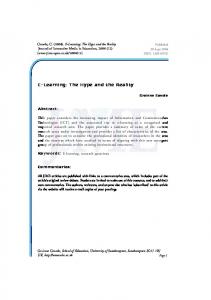
Our standard model has seven boxes of which six are in the upper 500m (Fig.1a). As is typical in box models (Watson and Garabato, 2006;Johnson et al., 2007), we assume a closed system that represents a zonally integrated ocean. Combining the Atlantic and Pacific into one basin is not ideal but the assumptions we shall make about latitudinal distributions of nutrients and export and where water upwells and sinks, hold in both basins. The SO is divided into an
5
Antarctic box and a sub-Antarctic box and the division is roughly at the polar front, assumed to be at 55oS. The low latitudes extend from 40oS to 40oN and are intersected by a narrow box, from 10oS to 10oN, which explicitly represents the high nutrient equatorial upwelling region. A northern box starts at 40oN and extends to the north pole. The volumes of the surface boxes are the same as in the real world between these specified zonal boundaries and for the deep box between 500m and the bottom. We shall use the term SO to describe both the Antarctic and the Sub-Antarctic boxes. In order to relate the model to the real world, we shall refer to the sinking in the Antarctic box as Antarctic Bottom Water (AABW).
The fluxes between the boxes are fully described by five independent model parameters: 1) Antarctic deep water formation, 2) northward surface Ekman transport between the SO surface boxes, 3) a southward transport representing the contribution of SO mesoscale eddies, 4) an equatorial upwelling flux, and 5) a northern upwelling flux. These variables are circled in Fig. 1a and the range of values they take is listed in Table 1. The rest of the transport terms are quantities derived from continuity. Note that the southward eddy flux is never more than the northward Ekman transport so that the residual flow into the equatorial box is always positive. Upwelling in the SO occurs in the Antarctic box (south of the polar front) and is equal to the net flow out of the box from Antarctic sinking and the residual circulation. In the northern box the upwelling is balanced by local downwelling so that it can be seen as a mixing term that brings up high nutrient water to the surface similar to winter mixing in the real ocean. The upwelling in the equatorial box represents both wind driven upwelling and that due to turbulent mixing. There is no simple way to represent the complex dynamics of the equatorial region – we have chosen to return the upwelled water in the northern box but in reality some downward mixing of the surface properties occurs locally and some of the upwelled water is subducted in the low latitudes. To ensure that our results are not highly dependent on equatorial upwelling or the northern sinking that goes along with it, the study is repeated in a model that does not have an equatorial box (Fig 1b). In this case the equatorial region is treated the same way as the low latitude regions. In another test of the effect of the geometry the upper layer depth was reduced from 500m to 300m. The soft tissue biological pump in our model is simplified to a one-nutrient formulation, P, assumed here to be phosphate (PO4). The nutrients are advected by the circulation in the usual way. Export production from a surface box is linearly proportional to the nutrient 6
concentration in the box. The proportionality constant, α, differs from box to box and encapsulates factors which limit the uptake of nutrients such as light or iron. It is referred to in the rest of the text as the nutrient utilization rate and is the fraction of the available nutrients that is
exported from the surface (rather than the fraction that is taken up in primary
production) each second. This constant is allowed to vary over a wide range of values (Table 1). The export production from the box is then simply, αP, multiplied by the volume of the box. The overall nutrient content is constrained to be the same as that derived from the World Ocean Atlas of 2005 (Garcia et al., 2006). The above model is mathematically formulated in the following seven equations,
Box A:
TAU PD – (TA + TT + αAVA) PA + TME PS = 0
Box S:
TT PA – (TT + αSVS) PS = 0
Box LS: Box E: Box LN: Box N: All:
(TT – TME) PS – (TT – TME + αLSVLS) PLS = 0 TEU PD + (TT – TME) PLS – (TT – TME + TEU + αEVE) PE = 0 (TT – TME + TEU) PE – (TT – TME + TEU + αLNVLN) PS = 0 TNU PD + (TT – TME+ TEU) PLN – (TT – TME + TEU + TNU + αNVN) PN = 0 VD PD + VA PA + VLS PLS+ VS PS + VE PE + VLN PLN+ VN PN = PSUM,
where T is a transport variable and V the box volume. The subscripts A, S, LS, E, LN, N, and D denote the Antarctic box, Sub-Antarctic box, Low latitude Southern box, Equatorial box, Low Latitude Northern box, Northern box, and Deep box respectively. Upwelling fluxes into the boxes have a U at the end, i.e., TAU is upwelling into the Antarctic box. The SO Ekman transport and mesoscale eddy transport are denoted by TT and TME respectively and PSUM is the total amount of PO4 molecules in the ocean. These equations are solved for 107 random combinations of the five circulation and five nutrient utilization input parameters. Note that the six surface boxes give only five nutrient utilization parameters because we assume that the conditions for biological production in the northern and southern low latitude boxes are similar and therefore set α to be the same in these regions (i.e., αLS = αLN )
7
3 3.1
Results The relation of preformed nutrients to the biological pump and atmospheric CO2
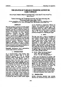
During glacial periods CO2 is drawn into the ocean through an increase in the surface to deep gradient of dissolved inorganic carbon (DIC). This gradient relies on the soft tissue biological pump which is the process in which carbon is being sequestrated into organic matter in the surface and later remineralized in the deep ocean. Nutrients that are advected to the deep ocean as a result of the physical circulation of the ocean are not available for biological uptake and are referred to as preformed nutrients. If the proportion of preformed nutrients in the deep ocean is large, the biological pump is inefficient, the vertical gradient of DIC weak, and the atmospheric CO2 high. The strong positive relation between preformed nutrients and atmospheric CO2 has been derived theoretically (Ito and Follows, 2005;Goodwin et al., 2008) and confirmed in ocean general circulation models (Ito and Follows, 2005;Marinov et al., 2006). We describe the biology in our model in terms of the macro nutrient PO4 and then use this connection to relate the preformed nutrient concentration to atmospheric CO2. The preformed nutrient concentration is defined as the fraction of nutrients that reach the deep ocean through the circulation multiplied by the deep ocean nutrient concentration. The biological pump efficiency is the fraction of nutrients that is exported to the deep ocean through biological productivity and ranges from near 0 to 100% for our 107 solutions (Fig 2). The preformed nutrient concentration ranges from 0 - 2.5 µmol Kg-1 and can be associated with a change in atmospheric CO2 of approximately 300 ppmv according to the theory of Ito and Follows (2005).
3.2
The interglacial states
It is common in carbon cycle box models to set the circulation as close as possible to observations or model output or to tune it to give realistic solutions (Keir, 1988;Toggweiler, 1999;Watson and Garabato, 2006). While these approaches have merit, it is not clear to which extent the conclusions of the studies depend on the chosen circulation states. In this study the whole parameter range is explored to ensure that our conclusions are not dependant on a chosen parameter. Initially 107 random solutions are calculated to cover all parameter
8
combinations within the limitations of our model setup. From these we select the modern states according to the circulation and nutrient and organic matter export distributions. In the first step, solutions are required to have higher export in the Sub-Antarctic than in the Antarctic box, and higher export in the equatorial box, northern and sub-Antarctic boxes than in the low latitude boxes. The circulation of the modern state is required to have at least 20 Sv (1 Sv = 106m3s-1) of northward Ekman transport and at least 5 Sv of AABW formation. Of the solutions that fulfil these criteria we consider the 300 solutions that best fit the modern phosphate distribution as derived from the World Ocean Atlas 2005 (Garcia et al., 2006). The maximum deviation from PO4 observations for any box of any of the 300 solutions is 0.3 µmol kg-1 (1 µmol =10-6 mol).
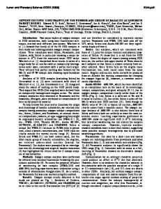
Figure 3 (top right) shows that these constraints can be explained using any among a wide range of input parameter sets. In this sense we effectively allow for model structural error using the plausibility approach of Holden et al. (2009;Edwards et al., 2010). The Ekman transport and AABW cover the whole range of permitted values in the 300 solutions. To satisfy the observations of high surface nutrients, the northern and equatorial upwelling fluxes are towards the higher range of their permitted values. The eddy mass flux is somewhat on the low side so that the average residual circulation of the interglacial parameter sets is about 16 Sv, with a minimum of 4 Sv. The wide range of circulation states already indicate that is may be wise not to pick one state on which to perform a sensitivity analysis and the conclusions drawn in this study are based on all these states rather than a single best guess. The interglacial nutrient utilization rates have more confined patterns than the circulation parameters. Low utilization rates in the AA region, the low latitudes, and the equatorial region are necessary to simulate modern phosphate distributions (Fig. 3, bottom right).
The purpose of isolating the best modern states is not to determine the real modern circulation or nutrient utilization. Rather, the modern states are obtained to 1) confirm that the model can reproduce a realistic interglacial state, 2) indicate the sensitivity of pCO2 and nutrient concentrations to the input parameters, given a modern state, and 3) provide reference states with which to compare the glacial states. The average efficiency of the biological pump of the 300 interglacial solutions is 35±4% which corresponds well with the estimate of 36% from Ito and Follows (2005). 9
3.3
The glacial states
Observations of the glacial ocean circulation are ambiguous but it is clear that the deep oceans were filled with a southern source water to a more shallow depth than today, and pore fluid measurements suggest this southern source water was much saltier than that from the North Atlantic (Ninnemann and Charles, 2002;Adkins et al., 2002b). Proxies for export production give a clearer picture than those for the circulation and indicate increased export in the SubAntarctic and Equatorial regions and reduced export in the Antarctic region (Kohfeld et al., 2005). It is uncertain by how much the export has changed in each region - we constrain the glacial solutions to those that have at least a 20% increase in export in the Sub-Antarctic and Equatorial region and a 20% decrease in the Antarctic box. The resulting states are only weakly dependent on this number (i.e., the percentage rate). From these we select the 300 that have the lowest preformed nutrients, i.e., the states that are associated with the greatest draw down of CO2 (Fig. 3, left ). The average preformed nutrient concentration, biopump efficiency, and pCO2 change for these states are 1.6 µmol kg-1 , 84%, and 165 ppmv respectively. To explain the glacial-interglacial change in pCO2 it is only necessary to account for a 100 ppmv change, though if the terrestrial biosphere was smaller in glacial time this might require a stronger marine drawdown to compensate. The more severe drawdown of CO2 illuminates clearly the parameters that are important for CO2 uptake, but our conclusions are qualitative and hold also for a weaker uptakes (confirmed, but not shown).
The circulation parameter which undergoes the greatest change in the glacial is the Antarctic bottom water (13 Sv average decrease), followed closely by mixing in the Northern high latitude regions (12 Sv average decrease). The northward Ekman transport is at least 13 Sv and on average 24 Sv. Interestingly, the southward eddy flux is never more than 20 Sv and always at least 9 Sv less than the Ekman transport (on average 18 Sv less, see section 4.3 for discussion). Equatorial upwelling can take on any value in the glacial. The nutrient utilization rate in the low latitudes or northern high latitude region are not very important in the glacial. However, the Antarctic nutrient utilization rate is low and the Equatorial and Sub-Antarctic utilization rates are high. The implications of the results are discussed in section 4. Note that
10
the average change can be viewed as the most likely change and the range gives the possible solutions that are consistent with the observations.
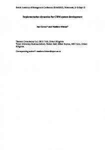
The glacial and interglacial states have so far been presented in terms of the input parameters and the preformed nutrients. The actual variables that are solved for are the phosphate concentrations. The average nutrient distribution for the 300 glacial states has a similar pattern to the interglacial although surface nutrients are reduced everywhere north of 40˚S (Fig. 4, top). The export production is higher by design in the Equatorial and Sub-Antarctic regions and lower in the Antarctic region of our modelled glacial states (Fig. 4, bottom). In the low latitudes we also find increased export which is consistent with the observations but this may well be fortuitous because the observations are in upwelling regions which we do not resolve in the model. The glacial states have a lower export production in the Northern region which is again consistent with the few data points north of 50˚N in the Kohfeld et al. (2005) reconstruction.
3.4
Sensitivity of preformed nutrients to circulation and nutrient utilization
In the previous section we determined which solutions are consistent with the proxies of export production and also give significantly decreased preformed nutrient concentrations in the deep ocean. This approach identifies what the possible combinations of circulation and nutrient utilization rates are that we need to look for in mechanisms to explain the glacial carbon cycle. It does not illustrate which of these parameters are responsible for the CO2 drawdown and which are only necessary to explain the proxy data of export production. For instance, it is likely that the reduced nutrient utilization rate in the glacial in the Antarctic regions (Fig. 3) is necessary to reduce export there and not to reduce preformed nutrients. Here we look at the sensitivity of the pCO2 and the export production (in regions that have constraints on the export) to the input parameters of the best fit interglacial state (Figs. 5, 6). The export flux and pCO2 are expressed as the difference from the export and pCO2 of the interglacial state. The sensitivities are dependent on the chosen reference state so we have also determined the sensitivity of pCO2 to input parameters for the other 299 interglacial states, for the 300 glacial states, and for 300 randomly chosen states from the complete set of solutions (Table 2). 11
From section 3.2 it is clear that the AABW formation, the northern mixing, and the equatorial upwelling are all less in the glacial states than in the interglacial states. Figure 5 shows that pCO2 is highly sensitive to the former two but indicates no great sensitivity of pCO2 to equatorial upwelling. However, if one considers all of the 300 interglacial and glacial states, the picture that emerges is different. The mean change in pCO2 due to a 15 Sv change in the upwelling is 16 ppmv in the interglacial and 30 ppmv in the glacial, almost half that of the AABW and northern upwelling (Table 2). The example indicates how misleading it can be to consider the importance of a carbon uptake mechanism only in a best guess fixed state (and this may very well be true for a control state in a numerical model too). The pCO2 has a weak negative relation to the eddy flux and is largely independent of the Ekman transport (Fig 5, Table 2). The atmospheric pCO2 is reduced when uptake of nutrients is more efficient in any of the surface regions in our model, but the sensitivity is highest north of 40°S (Fig. 6, Table 2). The best glacial states (i.e., those glacial states with lowest pCO2) have high nutrient utilization rates in all regions except the AA (Fig. 3). Here an increased utilization rate implies a higher export production (Fig. 6, top left) and that is not consistent with the observations. The surface transport is always from the south to the north so that biological productivity in the northern box does not influence the nutrient distributions or export in the other surface boxes. While it is clear that increased nutrient utilization in the low latitudes and northern regions helps to draw down CO2 (Table 2), the utilization parameters for these regions are not tightly grouped in the glacial states (Fig. 3). The lack of observations of export production here means that not enough information is available to indicate whether an increase in the nutrient utilization rate occurred.
3.5
The importance of the equatorial region
We have chosen in our control model to describe the equatorial region separately because a) this region behaves differently from the sub-tropics, b) there is a high number of export production observations here, and c) various hypotheses for glacial CO2 uptake revolve around this region. Including an equatorial upwelling flux is necessary to produce the high nutrient concentrations that are observed here. We have chosen, perhaps more for simplicity 12
that any other reason, to assume that the upwelled water all sinks to the deep ocean in the northern box. In the reality the dynamics in the equatorial region are complex and some of this upwelled water sinks out of the surface ocean in the sub-tropical gyres. Upwelling in the Equatorial regions is also sometimes modelled as a mixing (two-way) flux but in reality is it unlikely that there is a downwards transport of mass. The location of the sinking does not affect the nutrients in the equatorial region, but it does affect the dynamics in the boxes to its north. To ensure that the conclusions drawn from our results are not dependant on sensitive equatorial dynamics, we have repeated the analysis in a model in which the equatorial region has been removed (Fig. 1b). The concentration to which the low latitude phosphate is restored is the average phosphate concentration between 40˚S and 40˚N, excluding the equatorial regions between 10˚S and 10˚N. Naturally the glacial constraint of higher equatorial export production is also not applied.
The circulation and biological parameters that produce the best glacial and interglacial states (Fig. 7) are remarkably similar to those of the standard model that includes an equatorial region (Fig. 3). The only clearly noticeable difference is that the interglacial solutions are more tightly grouped and that the nutrient utilization in the sub-Antarctic and northern boxes are lower when no equatorial region exists. These are the regions where the highest export production occur. To compensate for the lack of upwelling of deep nutrients to the surface at the equator, the export from these two regions are reduced.
4
Implication for CO2 uptake
The main input parameters that are directly responsible for reduced atmospheric pCO2 in the glacial states of the model are AABW formation, northern mixing, and the nutrient utilization rates in the equatorial and low latitude regions (Figs. 3,5,6, Table 2). Perhaps surprisingly, the SO eddy fluxes and SO nutrient utilization rates are of secondary or no importance. We discuss the implication of each of our main glacial input parameter changes as well as those that are not as important as expected.
13
4.1
Reduction in AABW and northern mixing
Simulations of the ocean circulation during the Last Glacial Maximum give ambiguous results (Otto-Bliesner et al., 2007) but support observations that the boundary between North Atlantic and Southern Source deep water was shallower than today. Observations of δ13C, anoxic conditions in the deep SO, and reduced δ13N ratios in the glacial SO suggest that the ventilation was weaker there and the surface ocean more stratified (Francois et al., 1997;Hodell et al., 2003;Toggweiler et al., 2006). Sigman et al. (2004) proposed that the increased glacial stratification in the SO and North Pacific is a result of a drop in the mean ocean temperature. At very low temperatures the seawater density becomes almost insensitive to temperature changes and is mostly affected by salinity. In cold climates, heat loss becomes unable to destabilize polar haloclines, leading to a reduction in deep water formation. De Boer et al. (2007) tested the effect of cold water induced stratification in an ocean general circulation model and found that it was especially efficient in reducing convection in strong halocline regions such as the North Pacific and the SO. Such an effect could thus have been responsible for reducing AABW and northern mixing in the glacial ocean, as suggested by our model.
Another proposed mechanism for reducing AABW is reduced and northward shifted winds (Toggweiler et al., 2006). Note that the winds would not affect preformed nutrients through a reduced northward Ekman transport and associated upwelling but rather through the AA stratification that results from less wind-enhanced winter mixing and a consequent reduction in AABW formation. However, Sime et al. (submitted) have done an intensive atmospheric circulation study which strongly suggests that the SO winds were neither stronger nor shifted northward during the glacial and that the observations that have been interpreted as a northward wind shift can all be explained by sea surface temperature induced changes to the hydrological cycle.
An alternative explanation for reduced AABW formation during the last glacial that may have been active in conjunction with mean ocean temperature stratification is that destabilization of the water column was rare because of the extremely salty deep water (Adkins et al., 2002a). It is possible that the salty deep water formed through brine rejection in the Southern Ocean and was maintained by only a small amount of deep water formation. a small amount of deep 14
water formed in the SO as a result of brine rejection maintained the high density of the water in the deep ocean. The high vertical stratification could also have reduced the vertical mixing that might otherwise have caused the deep ocean water to decrease in density and rise to the surface (Watson and Garabato, 2006). The combination of very cold temperatures, salty deep water formed by brine rejection, and reduced deep mixing can explain a deep ocean filled with southern sourced water that nevertheless has very low rates of ventilation.
4.2
Increase in low latitude and equatorial export production
One proposed explanation for glacial oceanic uptake of CO2 is an increased dust supply to the Eastern Equatorial Pacific that invigorated the soft tissue pump (McGee et al., 2007;Winckler et al., 2008). This mechanism has been criticized due to observations of reduced opal accumulation rates in the region (Bradtmiller et al., 2006) but Pichevin et al. (2009) recently argued that the lower opal export can be explained by a decrease in the silicon to carbon uptake ratio in an iron rich environment. At first glance our model seems to support the concept of a global soft tissue pump being enhanced by a higher utilization of equatorial nutrients. However, it is not obvious that enhanced equatorial export would significantly decrease atmospheric CO2. The key to a global reduction in atmospheric CO2 through the soft tissue pump lies in the concentration of preformed nutrients in the deep ocean. Uptake of nutrients at the equator will only reduce deep ocean preformed nutrients if those nutrients would otherwise escape to a deep water formation region and be advected to the deep ocean in the physical circulation. This is unlikely to happen as ‘escaped’ nutrients have to pass through the low latitudes where the utilization is so high that surface nutrients are almost completely depleted. In our model the low latitude nutrients are not depleted because the nutrient concentration is averaged over a 500m deep upper layer. Hence nutrients leaving the equatorial region in our model interglacial states can reach the northern region unscathed and sink through advection there. This is indeed what happens as we find the nutrient concentration north of the equator much reduced for the glacial states (Fig. 4).
It is likely that the importance of the low latitude nutrient utilization in our glacial states is similarly exaggerated due to the fact that our surface ocean is 500m deep. In the real ocean, the nutrients in the interglacial surface ocean are almost completely depleted. A much larger 15
drawdown of nutrients, as suggested by our model for the glacial, is therefore unlikely. In spite of the fact that biological production is limited to the near surface of the ocean, say the top 100m, we have chosen a deeper level of 500m because the transport of Ekman and eddy flow and the resulting northward residual flow does not occur in euphotic zone only. Indeed, it is not possible to drive a realistic northward transport through surface boxes of 100m and maintain high gradients in surface nutrient concentrations.
To confirm that the high sensitivity of pCO2 to equatorial and low latitude nutrient utilization rates is exaggerated because of the assumption that the top 500m is biologically active, we reproduced our study in a model with an upper layer of 300m (Fig. 8). The meridional gradients in nutrient concentrations are very high at the ocean surface so that the solutions for the interglacial state in the shallow model are, as expected, not as close to the observations as in the standard model. The preformed nutrients are lower in the interglacial and it is more difficult for the ocean to take up CO2. As expected, the difference between the nutrient utilization in the glacial and interglacial states is much less pronounced than in the standard model (Fig. 8, bottom). We have argued that the importance of the nutrient utilization in the Equatorial region is likely to be exaggerated because any decrease in nutrients that are taken up in biological production there leads to an increase in the export production of the low latitude regions to which the nutrients escaped. However, the effect of equatorial production could be nonnegligible because, although nutrients in the surface low latitudes are almost completely depleted, nutrients can travel from the equator to the north in the sub-surface below the euphotic zone.
4.3
The Southern Ocean residual circulation
One of the leading hypotheses for glacial oceanic uptake of carbon is that of a reduced residual circulation in the Southern Ocean (Keeling and Visbeck, 2001;Watson and Garabato, 2006;Fischer et al., 2009). The residual circulation is the sum of the northward Ekman transport and the southward eddy fluxes and is controlled by the surface buoyancy forcing (Marshall and Radko, 2006). Reduced surface buoyancy input would lead to a reduced residual circulation and therefore reduced upwelling of nutrients and DIC to the surface. The 16
residence time of the nutrients in the surface is also expected to increase, enhancing the chances that they will be consumed in production rather than sink as preformed nutrients. The theory is reasonable but the processes involved in linking the residual circulation with the carbon cycle are complex and so far only one general circulation study that we know of has attempted to model it (Parekh et al., 2006). While a reduced upwelling of DIC rich water would reduce the outgassing of CO2 in the SO, it is possible that the reduced supply of nutrients to the surface will reduce the biological uptake of DIC by the same amount, leading to a reduction in the efficiency of the soft tissue pump so that the net effect on atmospheric CO2 is zero. Another complication is the effect of the reduced nutrients on the productivity in the SO. If the water masses in the upper and lower branch of the overturning in the ACC are mostly separated and the upper branch is associated with the residual circulation, then one would expect that the reduced surface nutrients would affect the Sub-Antarctic region north of the polar front more than the Antarctic region to the south. The distinction is important because a reduction in nutrients to the south would reduce the deep ocean preformed nutrient transported by AABW while at the north it would only affect the export in the Sub-Antarctic region and probably not the CO2. The residence time of the nutrients in the SO may affect their chance of being biologically consumed rather than becoming preformed nutrients but again, one would expect this to be important in the Antarctic region where observations show no indication of increased export. To complicate things further, the strength of deep mixing in the Antarctic regions and AABW formation is not necessarily related to the residual circulation but would modulate its influence.
Parekh et al. (2006) tested the affect of the residual circulation on atmospheric CO2 in a general circulation model coupled to a carbon cycle model. They found a drop in atmospheric pCO2 of about 3ppmv per Sverdrup reduction in the residual circulation. However, they changed the residual circulation by adjusting the winds in the SO from 50% to 150% of modern winds. An increase in the SO winds would indeed increase the residual circulation if the buoyancy flux is not fixed, but it would probably also decrease the stratification further south and increase AABW formation (De Boer et al., 2008). Our results suggest that the observed reduction in atmospheric CO2 for weaker winds was a consequence of the reduced preformed nutrients due to reduced AABW formation in their model rather than a weaker residual circulation. Also, a reduction in the residual circulation due to weakened winds will
17
have a different effect than the more likely case in which the winds are the same but the SO eddies increased. In the former case there will be little mixing of nutrients across the ACC while in the latter case the strong winds and eddies will result in more cross frontal mixing of nutrients.
In our model we explore the effect of the residual circulation beyond that of conceptual deductions and furthermore, unlike what is possible in GCMs, we isolate the various processes that play a role in the region. Thus, we change the residual circulation by changing the eddy fluxes or the Ekman transport without changing the AABW formation and we increase or decrease the nutrient utilization rate in both the Antarctic and Sub-Antarctic regions in conjunction with the residual circulation changes or separately. What we find is that a strongly reduced residual circulation (strong southward eddy fluxes countering the Ekman flow) is neither necessary nor sufficient to explain the glacial state (Fig. 4). In fact, the residual circulation is 18 ± 4 Sv in the glacial states as compared to 16 ± 6 Sv in the interglacial states. The range for the glacial is 9 to 29 Sv and for the interglacial 4 to 29 Sv indicating that in none of the glacial states is the residual circulation less than 9 Sv. The result is interesting because the pCO2 shows a weak but clear negative correlation with the eddy flux (Table 2) so that one would expect higher eddy transport in the glacial. The curiosity is explained when one drops the requirement for higher sub-Antarctic export production. In this case the eddy flux still does not increase much (remains 9 Sv on average), but the Ekman transport drops from 25 Sv to 9 Sv (and the soft tissue pump efficiency shoots to 95%). It is the requirement of enhanced sub-AA production that forces the residual circulation to supply nutrients for export production.
4.4
The Southern Ocean nutrient utilization and the biochemical divide
It has been proposed that the polar front divides the Southern Ocean into a Sub-Antarctic region where increased biological productivity results in increased export but not oceanic uptake of CO2 and an Antarctic region where it does take up CO2 (Marinov et al. 2006). We also find in our model that increased nutrient utilization is slightly more effective at reducing atmospheric CO2 in the Antarctic than in the Sub-Antarctic in our interglacial states (Fig. 6, Table 2). However, increased Antarctic nutrient uptake leads to a large increase in export 18
production there and a decrease in export from the Sub-Antarctic while the observations point clearly to the opposite effect. On the other hand, the observations are not violated by an increased export from the Sub-Antarctic region. While its effect on atmospheric CO2 is not huge compared to other mechanisms, it may have been responsible for some of the smaller variations in the glacial CO2 record. In the glacial states the nutrient utilization is much decreased in both regions and of a similar magnitude. Overall our model suggests that one must look for changes in the circulation rather than the biology to explain the strong link between the SO temperature and atmospheric CO2 in the ice core record..
5
Conclusions
We have formulated a simple box model that encapsulates the major circulation variables of the real ocean and explores the effect of nutrient utilization in each of the major biological production regimes. Due to the simplicity of the model we could explore the full parameters space which includes five circulation and five nutrient utilization rate parameters to produce 107 solutions. Of these solutions, we determined the subsets which best fit the current observations and those that fulfil the glacial observations. In addition, we explored the sensitivity of deep ocean preformed nutrients (and by deduction the atmospheric pCO2) and export production to each input parameter separately.
The strong link between temperature and CO2 in the Vostok and Epica ice core records suggest that the SO must be a player in the glacial carbon cycle. Our model suggests the SOCO2 link is through a change in AABW formation or SO deep mixing and not through changes in residual circulation or the biology directly. Such a reduction in AABW can be brought on by increased surface stratification that inhibits convection and deep mixing or increased deep stratification that reduces vertical mixing and upwelling of AABW. The surface stratification would have been enhanced due to the near freezing water temperature at which the density is not very sensitive to temperature and thus haloclines are not easily overturned in winter. This type of stratification was probably also active in the North Pacific and to a lesser extent the North Atlantic and may have contributed to further uptake of CO2 through reduced mixing as suggested by our model. A decrease in SO winds would also lead to increased stratification although recent work by Sime et al. (submitted) suggest that it is unlikely that the winds weakened or shifted much during the glacial. 19
A reduced residual circulation through increased southward eddy fluxes is one of the leading hypotheses for glacial CO2 uptake. The atmospheric CO2 is only weakly sensitive to the SO residual circulation in the model. All the glacial solutions have a residual circulation of at least 9 Sv and it can be as high as 30 Sv. Further analysis indicated that this is because of the observational constraint of higher export production in the sub-AA region. The implication is that the sub-AA production is not only controlled by the nutrient utilization rate, but is also limited by the supply of nutrients. The extent to which this is true in the glacial ocean is unclear. The reason why the residual circulation in itself affects the atmospheric CO2 only weakly can be understood in terms of the productive and unproductive circulation conceptualization of Toggweiler et al. (2003b;2006). The productive circulation represents the North Atlantic overturning cell and the unproductive circulation the AABW cell. Nutrients that upwell in the SO are transported northward in the Atlantic or Pacific will be consumed before they reach the North Atlantic deep water formation region and thus all the associated DIC that was outgassed at their surfacing is subsequently taken up again. The circulation therefore has no net effect on atmospheric CO2. In the unproductive southern circulation, upwelled nutrients are not depleted by the time they reach the AABW formation region and this branch is thus less productive in terms of the biological pump. A reduction in the residual circulation will indeed reduce upwelling, but it will reduce only the productive circulation to which atmospheric CO2 is less sensitive. It may affect the nutrient supply and utilization in the SO though.
The biology of the SO does not emerge as a directly important player in the biological pump. The deep ocean preformed nutrient concentration is more sensitive to changes in the nutrient utilization north of 40oS. We do find a weak biochemical divide (similar to Marinov et al. (2006)) in the sense that nutrient uptake in the sub-AA draws down a bit less CO2 than in the AA. It appears irrelevant though because an increase in the AA nutrient utilization leads to higher export production in the region and that is counter to the observations. The strong link between atmospheric CO2 and temperature in Antarctic ice core records has been put forward as indicating that the SO must have played an important role in the glacial carbon cycle. Our study suggest that this link is through changes in deep mixing and AABW formation in the Antarctic region and not through changes in biology of the SO or the residual circulation. 20
Sub-Antarctic productivity enhanced by a supply of iron may have accounted for smaller variations in the glacial CO2 record.
The equatorial region emerges from our model results as an important region for glacial CO2 uptake. While there may be some real sensitivity here, one should keep in mind that the dynamics are not well resolved and the sensitivity of the equatorial and low latitude regions are exaggerated due to the fact that the biologically active upper layer in the model is 500m deep. The low latitude nutrients are therefore not depleted and nutrients can easily escape from the equatorial region to the northern region where it can sink as preformed nutrients. We confirmed that deep ocean preformed nutrients are less sensitive to increased production in the equatorial and low latitude regions in a shallower upper layer version of the model.
The model is simple by construction. The conclusions drawn from it are qualitative in nature and, as with all models, should be interpreted within its limitations. However, unlike General Circulation Models and many box models, our approach to cover the whole of parameter space means that there are no tuned parameters in the model. Rather, all input parameters are deduced from observations or are variables that are explored as part of the solution. It may be a useful approach to adopt in future box model studies of the carbon cycle. Suggestions for further refinements to the model are to divide the deep ocean into an upper and lower box which are fed from the north and south respectively, to separate the Atlantic and Pacific basins, and to improve the Equatorial dynamics. The addition of a carbonate pump would also provide further insight.
Acknowledgements This work was funded by NERC Quaternary Quest Fellowship NE/D001803/1. . NRE acknowledges support from NERC RAPID and NERC DESIRE projects.
21
Tables Table 1: Model parameters for the standard 7 box model. The volumes and observed PO4 concentrations are derived from the World Ocean Atlas 2006. Volume
Observed PO4
α
Transport
(1015m3)
(10-6 µmol kg-
(10-10 s-1)
(106 m3s-1)
1
)
Antarctic
16
2.45
0 - 10
AABW
0 – 20
Sub-Antarctic
21
1.70
0 - 10
Ekman
0 – 30
Low lat - south
47
1.04
0 - 10
SO eddies
0 – 30
Equator
32
1.89
0 - 10
EQ
0 – 20
upwelling Low lat - north
36
1.23
0 - 10
Northern
0 - 20
upwelling North Deep Ocean
16
1.60
1300
2.64
0 - 10
22
Table 2: The mean and standard deviation of the change in pCO2 due to a change in the input parameters for the 300 glacial and interglacial states, and for 300 randomly chosen states. For the circulation parameter the difference in pCO2 due to a change in the circulation from 5 to 20 Sv is shown and for the nutrient utilization the difference in pCO2 due to a change in α from 2 to 8e-10 s-1 Circulation
Glacial
Interglacial
Random
(ppm/15Sv)
(ppm/15Sv)
(ppm/15Sv)
AABW
73 ± 6
26 ± 5
44 ± 20
Ekman
5 ± 12
0± 5
-7 ± 16
Eddies
-10 ± 8
11 ± 4
0 ± 12
Eq-upwell
30 ± 8
16 ± 6
4 ± 20
North-mix
67 ± 7
25 ± 4
52 ± 18
Uptake efficiency
Glacial
Interglacial
Random
(ppm/6x1010s-1)
(ppm/6x1010s-1)
(ppm/6x1010s-1)
AA
-5 ± 2
-20 ± 3
-20 ± 10
Sub-AA
-6 ± 3
-16 ± 3
-7 ± 5
Low lats
-27 ± 7
-34 ± 6
-19 ± 12
Equatorial
-17 ± 4
-28 ± 4
-14 ± 10
Northern
-14 ± 4
-33 ± 4
-31 ± 13
23
Figures
Fig. 1: The control model consists of 7 upper boxes above 500m and one deep box (a). Export production is denoted by the dotted arrows and is the product of the nutrients concentration and a nutrient utilization rate that varies for each surface box (see text for details). The flow of water between the boxes (solid thick arrows) has five dimensions of freedom and we have varied the transports that are circled. The other transports are derived from these and conservations of mass. A second model is presented in which the equatorial region has been integrated into the low latitude boxes (b).
24
Fig 2: The atmospheric CO2 in the model as a function of the preformed nutrients for all 107 solutions (left axis) as calculated according to the theory of Ito and Follows (2005). A zero pCO2 is assumed at the average preformed nutrient concentration of our 300 best interglacial solutions (see section 3.2 for an explanation of how these are derived). The pCO2 and preformed nutrients are also linearly related to the efficiency of the biological pump (right axis).
25
Fig. 3: The circulation (top) and nutrient utilization rate (bottom) parameters of the interglacial states (right) and the glacial states (left) are shown here against the preformed nutrient concentration in the deep ocean. The top axis relates the difference in preformed nutrient between the glacial and interglacial states to changes in atmospheric pCO2 (as discussed in section 3.1). Best fit lines are drawn through the solutions for visual aid. They do not imply an independent linear correlation between the preformed nutrient concentrations and the input parameters.
26
Fig. 4: The average surface nutrient concentrations (top) for the 300 interglacial states (solid red) and the 300 glacial states (solid blue). Also shown for reference is the observed modern nutrient distribution (dashed red). Export production (bottom) from each surface box for the interglacial and glacial states. The modern nutrient distribution were obtained from the World Ocean Atlas (Garcia et al., 2006).
27
Fig 5: The response of atmospheric pCO2 (solid black), Antarctic export production (solid dark blue), Sub-Antarctic export production (dashed magneta), and Equatorial export production (dashed light blue) to the five circulation input parameters. The export fluxes (left axis) and pCO2 (right axis) are expressed as the difference from that of the best fit interglacial change.
28
Fig 6: Same as Fig. 5 but here the sensitivity of the export production and pCO2 to the nutrient utilization rate parameters are explored.
29
Fig 7: Same as Fig. 3 but for the model without an equatorial region.
30
Fig 8: Same as Fig. 3 but for the division between the upper and deep ocean is at 300m in stead of the standard 500m.
31
References Adkins, J. F., McIntyre, K., and Schrag, D. P.: The salinity, temperature, and delta O-18 of the glacial deep ocean, Science, 298, 1769-1773, 2002a. Adkins, J. F., McIntyre, K., and Schrag, D. P.: The temperature, salinity and delta O-18 of the LGM deep ocean, Geochim Cosmochim Ac, 66, A7-a7, 2002b. Anderson, R. F., Ali, S., Bradtmiller, L. I., Nielsen, S. H. H., Fleisher, M. Q., Anderson, B. E., and Burckle, L. H.: Wind-Driven Upwelling in the Southern Ocean and the Deglacial Rise in Atmospheric CO2, Science, 323, 1443-1448, 2009. Augustin, L., Barbante, C., Barnes, P. R. F., Barnola, J. M., Bigler, M., Castellano, E., Cattani, O., Chappellaz, J., DahlJensen, D., Delmonte, B., Dreyfus, G., Durand, G., Falourd, S., Fischer, H., Fluckiger, J., Hansson, M. E., Huybrechts, P., Jugie, R., Johnsen, S. J., Jouzel, J., Kaufmann, P., Kipfstuhl, J., Lambert, F., Lipenkov, V. Y., Littot, G. V. C., Longinelli, A., Lorrain, R., Maggi, V., Masson-Delmotte, V., Miller, H., Mulvaney, R., Oerlemans, J., Oerter, H., Orombelli, G., Parrenin, F., Peel, D. A., Petit, J. R., Raynaud, D., Ritz, C., Ruth, U., Schwander, J., Siegenthaler, U., Souchez, R., Stauffer, B., Steffensen, J. P., Stenni, B., Stocker, T. F., Tabacco, I. E., Udisti, R., van de Wal, R. S. W., van den Broeke, M., Weiss, J., Wilhelms, F., Winther, J. G., Wolff, E. W., Zucchelli, M., and Members, E. C.: Eight glacial cycles from an Antarctic ice core, Nature, 429, 623-628, 2004. Bradtmiller, L. I., Anderson, R. F., Fleisher, M. Q., and Burckle, L. H.: Diatom productivity in the equatorial Pacific Ocean from the last glacial period to the present: A test of the silicic acid leakage hypothesis, Paleoceanography, 21, -, 2006. Brovkin, V., Ganopolski, A., Archer, D., and Rahmstorf, S.: Lowering of glacial atmospheric CO2 in response to changes in oceanic circulation and marine biogeochemistry, Paleoceanography, 22, -, 2007. De Boer, A. M., Sigman, D. M., Toggweiler, J. R., and Russell, J. L.: Effect of global ocean temperature change on deep ocean ventilation, Paleoceanography, 22, 2007. De Boer, A. M., Toggweiler, J. R., and Sigman, D. M.: Atlantic dominance of the meridional overturning circulation, Journal of Physical Oceanography, 38, 435-450, 2008. De Pol-Holz, R., Keigwin, L., Southon, J., Hebbeln, D., and Mohtadi, M.: No signature of abyssal carbon in intermediate waters off Chile during deglaciation, Nat Geosci, 3, 192-195, 2010. Edwards, N. R., Cameron, D., and Rougier, J.: Precalibrating an intermediate complexity climate model, Clim Dynam, submitted, 2010. Fischer, M., Schmitt, J., Luthi, D., Stocker, T. F., Tschumi, T., Parekh, P., Joos, F., Kohler, P., and Volker, C.: The role of Southern Ocean processes on orbital and millennial CO2 variations - A synthesis, Quaternary Sci Rev, 2009. Francois, R., Altabet, M. A., Yu, E. F., Sigman, D. M., Bacon, M. P., Frank, M., Bohrmann, G., Bareille, G., and Labeyrie, L. D.: Contribution of Southern Ocean surfacewater stratification to low atmospheric CO2 concentrations during the last glacial period, Nature, 389, 929-935, 1997. Garcia, H. E., Locarnini, R. A., Boyer, T. P., and Antonov, J. I.: World Ocean Atlas 2005, Volume 4: Nutrients (phosphate, nitrate, silicate), NOAA Atlas NESDIS 64, edited by: Levitus, S., U.S. Government Printing Office, Washington, D.C., 396 pp., 2006. 32
Goodwin, P., Follows, M. J., and Williams, R. G.: Analytical relationships between atmospheric carbon dioxide, carbon emissions, and ocean processes, Global Biogeochem Cy, 22, -, 2008. Hodell, D. A., Venz, K. A., Charles, C. D., and Ninnemann, U. S.: Pleistocene vertical carbon isotope and carbonate gradients in the South Atlantic sector of the Southern Ocean, Geochem Geophy Geosy, 4, -, 2003. Holden, P. B., Edwards, N. R., Oliver, K. I. C., Lenton, T. M., and Wilkinson, R. D.: A probabilistic calibration of climate sensitivity and terrestrial carbon change in GENIE-1, Clim Dynam, doi: 10.1007/s00382-009-0630-8 2009. Ito, T., and Follows, M. J.: Preformed phosphate, soft tissue pump and atmospheric CO2, Journal of Marine Research, 63, 813-839, 2005. Johnson, H. L., Marshall, D. P., and Sprowson, D. A. J.: Reconciling theories of a mechanically driven meridional overturning circulation with thermohaline forcing and multiple equilibria, Clim Dynam, 29, 821-836, 2007. Joos, F., Sarmiento, J. L., and Siegenthaler, U.: Estimates of the Effect of Southern-Ocean Iron Fertilization on Atmospheric Co2 Concentrations, Nature, 349, 772-775, 1991. Karsten, R. H., and Marshall, J.: Constructing the residual circulation of the ACC from observations, Journal of Physical Oceanography, 32, 3315-3327, 2002. Keeling, R. F., and Visbeck, M.: Palaeoceanography - Antarctic stratification and glacial CO2, Nature, 412, 605-606, 2001. Keir, R. S.: On the Pleistocene ocean ocean geochemistry and circulation, Paleoceanography, 3, 413-445, 1988. Kohfeld, K. E., Le Quere, C., Harrison, S. P., and Anderson, R. F.: Role of marine biology in glacial-interglacial CO2 cycles, Science, 308, 74-78, 2005. Luthi, D., Le Floch, M., Bereiter, B., Blunier, T., Barnola, J. M., Siegenthaler, U., Raynaud, D., Jouzel, J., Fischer, H., Kawamura, K., and Stocker, T. F.: High-resolution carbon dioxide concentration record 650,000-800,000 years before present, Nature, 453, 379382, 2008. Marinov, I., Gnanadesikan, A., Toggweiler, J. R., and Sarmiento, J. L.: The Southern Ocean biogeochemical divide, Nature, 441, 964-967, 2006. Marshall, J., and Radko, T.: Residual-mean solutions for the Antarctic Circumpolar Current and its associated overturning circulation, Journal of Physical Oceanography, 33, 2341-2354, 2003. Marshall, J., and Radko, T.: A model of the upper branch of the meridional overturning of the southern ocean, Prog Oceanogr, 70, 331-345, 2006. Matsumoto, K., Oba, T., Lynch-Stieglitz, J., and Yamamoto, H.: Interior hydrography and circulation of the glacial Pacific Ocean, Quaternary Sci Rev, 21, 1693-1704, 2002. McGee, D., Marcantonio, F., and Lynch-Stieglitz, J.: Deglacial changes in dust flux in the eastern equatorial Pacific, Earth Planet Sc Lett, 257, 215-230, 2007. Ninnemann, U. S., and Charles, C. D.: Changes in the mode of Southern Ocean circulation over the last glacial cycle revealed by foraminiferal stable isotopic variability, Earth Planet Sc Lett, 201, 383-396, 2002. 33
Otto-Bliesner, B. L., Hewitt, C. D., Marchitto, T. M., Brady, E., Abe-Ouchi, A., Crucifix, M., Murakami, S., and Weber, S. L.: Last Glacial Maximum ocean thermohaline circulation: PMIP2 model intercomparisons and data constraints, Geophys Res Lett, 34, -, 2007. Parekh, P., Follows, M. J., Dutkiewicz, S., and Ito, T.: Physical and biological regulation of the soft tissue carbon pump, Paleoceanography, 21, -, 2006. Parekh, P., Joos, F., and Muller, S. A.: A modeling assessment of the interplay between aeolian iron fluxes and iron-binding ligands in controlling carbon dioxide fluctuations during Antarctic warm events, Paleoceanography, 23, -, 2008. Petit, J. R., Jouzel, J., Raynaud, D., Barkov, N. I., Barnola, J. M., Basile, I., Bender, M., Chappellaz, J., Davis, M., Delaygue, G., Delmotte, M., Kotlyakov, V. M., Legrand, M., Lipenkov, V. Y., Lorius, C., Pepin, L., Ritz, C., Saltzman, E., and Stievenard, M.: Climate and atmospheric history of the past 420,000 years from the Vostok ice core, Antarctica, Nature, 399, 429-436, 1999. Pichevin, L. E., Reynolds, B. C., Ganeshram, R. S., Cacho, I., Pena, L., Keefe, K., and Ellam, R. M.: Enhanced carbon pump inferred from relaxation of nutrient limitation in the glacial ocean, Nature, 459, 1114-U1198, 2009. Sarmiento, J. L., and Toggweiler, J. R.: A New Model for the Role of the Oceans in Determining Atmospheric Pco2, Nature, 308, 621-624, 1984. Siegenthaler, U., Monnin, E., Kawamura, K., Spahni, R., Schwander, J., Stauffer, B., Stocker, T. F., Barnola, J. M., and Fischer, H.: Supporting evidence from the EPICA Dronning Maud Land ice core for atmospheric CO2 changes during the past millennium, Tellus B, 57, 51-57, 2005. Sigman, D. M., and Boyle, E. A.: Palaeoceanography - Antarctic stratification and glacial CO2 - Sigman and Boyle reply, Nature, 412, 606-606, 2001. Sigman, D. M., Jaccard, S. L., and Haug, G. H.: Polar ocean stratification in a cold climate, Nature, 428, 59-63, 2004. Toggweiler, J. R.: Variation of atmospheric CO2 by ventilation of the ocean's deepest water, Paleoceanography, 14, 571-588, 1999. Toggweiler, J. R., Gnanadesikan, A., Carson, S., Murnane, R., and Sarmiento, J. L.: Representation of the carbon cycle in box models and GCMs: 1. Solubility pump, Global Biogeochem Cy, 17, -, 2003a. Toggweiler, J. R., Murnane, R., Carson, S., Gnanadesikan, A., and Sarmiento, J. L.: Representation of the carbon cycle in box models and GCMs - 2. Organic pump, Global Biogeochem Cy, 17, -, 2003b. Toggweiler, J. R., Russel, J. L., and Carson, S. R.: The Mid-Latitude Westerlies, Atmospheric CO2, and Climate Change during the Ice Ages., Paleoceanography, 21, 2006. Watson, A. J., Bakker, D. C. E., Ridgwell, A. J., Boyd, P. W., and Law, C. S.: Effect of iron supply on Southern Ocean CO2 uptake and implications for glacial atmospheric CO2, Nature, 407, 730-733, 2000. Watson, A. J., and Garabato, A. C. N.: The role of Southern Ocean mixing and upwelling in glacial-interglacial atmospheric CO2 change, Tellus B, 58, 73-87, 2006.
34
Winckler, G., Anderson, R. F., Fleisher, M. Q., Mcgee, D., and Mahowald, N.: Covariant glacial-interglacial dust fluxes in the equatorial Pacific and Antarctica, Science, 320, 93-96, 2008.
35