well below high performance graphics stations such as a Silicon Graphics In- ..... erty, shire or state, likewise a theoretician will be able to compare several ...
ADVISE Agricultural Developmental Visualisation Interactive Software Environment L. Lau1 , M. Rezny1, J. Belward1, K. Burrage1 and B. Pohl2
Research Report No. 94-03 July 1994 Seminar f ur Angewandte Mathematik Eidgen ossische Technische Hochschule CH-8092 Z urich Switzerland 1 2
Department of Mathematics, University of Queensland, Brisbane 4072, Australia. Seminar f�ur Angewandte Mathematik, ETH Z�urich, 8092 Z�urich, Switzerland.
ADVISE Agricultural Developmental Visualisation Interactive Software Environment L. Lau1 , M. Rezny1, J. Belward1, K. Burrage1 and B. Pohl2 Seminar f ur Angewandte Mathematik Eidgen ossische Technische Hochschule CH-8092 Z urich Switzerland Research Report No. 94-03
July 1994
Abstract
The quantum increase in computing power provided by contemporary parallel architectures o�ers the opportunity to confront problems of ever increasing complexity and size. With these developments new problems arise in techniques for the manipulation, transmission and display of large data sets as they occur for example in environmental modelling. The hardware and software of modern graphical display devices has the potential to enable large data sets to be presented in compact and informative con�gurations. The problem addressed here is to how to match these resources in an optimal way. The analysis of environmental models, for instance, is signi�cantly aided by visualisation, however when large data structures need to be analysed the static nature of the data causes large communication overheads. Similarly if a dynamic approach is taken, while CPU power and large memory capacity may be available, communication between the computing resource and the display device can impair the development and analysis of the model. Treated as a single integrated unit such a system is likely to lead to unwieldy code which is di�cult to maintain and re�ne. We present here a package, ADVISE, which acts as a communication interface between the client, typically a graphics device, and the server, a computing resource such as a vector supercomputer, a parallel computer or some network of machines. The approach taken is that the information system comprises three component parts, those of client, server and interface. The interface is an object of su�cient sophistication to permit the use and development of each of the client and server modules separately. Further, multiple distinct jobs may be run simultaneously for multiple clients.
Keywords: Client-server, environmental modelling, visualization Subject Classi�cation: 68B99, 68K05, 68J10 1 2
Department of Mathematics, University of Queensland, Brisbane 4072, Australia. Seminar f�ur Angewandte Mathematik, ETH Z�urich, 8092 Z�urich, Switzerland.
1 Background: Australia and El Ni~no Australia, the sixth largest country on Earth, covers an area of nearly 8,000,000 km2. This continent is bounded by latitudes 10o and 44o south and stretches nearly 4000 km from south to north and 4300 km from west to east. Most of the Australian population of 17 million people live in a narrow coastal belt 200 km wide along the southern and eastern seaboard. Queensland, the second largest state, is situated in the north{eastern part of Australia. Two of the country's (and Queensland's) major physiographic regions are the Great Artesian Basin and the Great Dividing Range1. Most of the Great Artesian Basin receives an annual rainfall of less than 400 mm and an annual rainfall of less than 250 mm is common in many regions. In fact, over two thirds of Australia's landmass receives less than 500 mm of rainfall a year and over one third receives less than 250 mm of rainfall a year. In Queensland, annual rainfall ranges from 4500 mm on the north{east coast to 100 mm in the arid south{west and as a consequence, conditions in summer2 are hot and humid on the coast, and hot and dry inland. This dramatic decrease in rainfall as one moves inland results in frequent droughts, which are exacerbated by violent storms and occasional serious �ooding over the vast inland plain. The inland plains form one of the great natural grasslands of the world and the water stored in the Great Arterial Basin underlying the plains is pumped to the surface to provide water for livestock. Most of Australia's arable land lies along the eastern coast, while in inland Queensland the major industries are beef and grain. Arable land totals about 6% (480,000 km2) of the total land area of Australia and, of that, one third requires irrigation3. In certain years there is a weakening of atmospheric circulation and the strong south{east trade winds o� the west coast of South America fade. These conditions allow a stream of the Paci�c Equatorial Counter{current to shift south by as much as 10o of latitude. This phenomenon has been called El Ni~no (the child, in Spanish) as it often occurs at Christmas. Notable occurrences were in 1891, 1925, 1953, 1983 and most recently in 1991. The arrival of El Ni~no signals a tremendous increase in rainfall on the usually arid western coast of South America and drought conditions over Australia. As an example, there are some regions of western Queensland which have had no measurable rainfall for over 28 months. The recent El Ni~no e�ect is estimated to have already caused an economic loss to Queensland in excess of one billion dollars. Thus it can be seen that the accurate and e�cient monitoring and subsequent modelling of drought conditions, provides the basis for a decision support system, which could have enormous �nancial and social bene�ts for Australia. A complex series of high ridges, high plains and plateaus in eastern Australia extending from the very north to the very south of the continent 2 December to February 3 This area of 160,000 km2 is approximately twice the size of Austria. 1
1
2 Environmental models The Queensland Department of Primary Industries (QDPI) has developed a model for modelling the e�ects of climate on pasture growth and subsequent stock growth. This was initially implemented as a point model, i.e. it models a homogeneous area of soil and pasture as one single point. The point model can be extended to become a spatial model over two spatial dimensions and run over a non{homogeneous area such as Queensland, in the following way: Firstly, the area is discretised into a set of small rectangular regions. Point estimates are then determined for each of the static parameters in each of these regions. This is done by �eld testing and the use of satellite images. Climate data is collected daily or weekly from up to 3000 meteorological stations scattered across Queensland. Secondly, surfaces are estimated for each of these climate variables for each day over which the model will be run. Point estimates for each region are then calculated from these surfaces. Lastly, given an initial state vector for each region, an independent simulation is then run for each of these regions. This spatial model consists of two separate FORTRAN77 programs: a surface �tting code and a pasture model. The surface �tting code computes an accurate interpolation of collected data (such as rainfall) using a cross{validation algorithm due to �?]. The �nal stage of this code interpolates this surface over an equidistant grid, which is superimposed on the map of Queensland. Six such surfaces4 are then used as the climate input data for the pasture model. This model currently simulates 12 physical parameters relating to daily environmental and pastoral conditions over a period of one year. The daily values of these parameters are then output to a storage medium for subsequent processing and analysis. A rectangular grid with an equidistant resolution of 10 km over Queensland has 29016 elements. To model the pasture growth on this grid for one year requires over 107 simulations, which takes about 12 minutes to run on a Sun SPARC2. We have also reported elsewhere �?] the use of these two codes as benchmarks for the assessment of various parallel, vector and distributed systems. We now routinely run this model on a 4096 processor Maspar MP1, a Cray YMP/2D and a network of up to 20 workstations of varying type and performance all situated at the University of Queensland. Moreover, in order to obtain a more realistic and accurate model QDPI would like to extend the model to cover Australia at 2.5 km grid resolution which would result in a one hundred fold increase in computational requirements. It is also required to run the model over much longer time frames than a single year. It is envisaged to extend this model to allow economic impact to be taken into account when making resource management decisions. It has been estimated that if the pasture model is run over Australia with this increased resolution using the 100 years of existing weather data, it would take approximately 2000 hours of CPU time on a Sun SPARC2. Even on the Cray YMP/2D it would take about 10 hours running at its peak performance of 666 MFlops. 4
Rainfall, maximum and minimum temperature, vapour pressure, evaporation and radiation
2
The computing demands which arise from the use of the pasture maps are the consequence of the need to simulate future possible situations and to compare several di�erent outcomes. The model may be required to run with an initial set of parameter values, halted and started and perhaps restarted several times from that point with di�erent sets of parameters. Thus the modelling environment needs to be interactive. This contrasts with a GIS system in which variations on the information to be displayed are limited to the content of the database. These remarks suggest that the traditional approach to modelling and interaction with large data sets needs to be revised. In the traditional approach a spatial model is run on a high performance computer and the required data stored in �les, which can then be visualised on the user's workstation using existing visualisation or GIS packages. The disadvantages with this approach are that: 1. The complete sets of parameters to be viewed must be speci�ed in advance, with a concomitant creation of many large data �les to make sure that all parameters that may be of interest are available for analysis. 2. These large data sets should be output as binary �les for e�ciency reasons. But, due to data representation di�erences between various architectures, data must either be further processed through data conversion programs or stored in a less e�cient but portable ASCII format. 3. There is no interaction possible with the simulation. The typical modelling process is to run the simulation, possibly transfer or process the data �les, analyse these �les, modify the parameters of interest and then, as necessary, re{iterate this process. Thus, at each iteration, a large amount of (possibly unnecessary) information is created and has to be transfered or processed. Furthermore, the entire simulation has to be performed, although subsequent analysis after only a few steps of the model may have already determined a poor choice of parameters. Finally, this approach does not allow the user to interactively modify parameters during the course of the simulation. Environmental models are important because they can provide the basis for ef�cient management of agricultural resources, especially during di�cult climatic periods such as drought. Good visualisation techniques allow the resource manager to easily inspect the e�ects of tentative management decisions. Moreover, fast response times increase the number of options that can be modelled in a given time frame. These improvements enhance the chances of making more informed decisions.
3 Motivation for ADVISE In order to be able to accomplish these goals, a collaborative arrangement has been formed between the Centre for Industrial Mathematics and Parallel Computing (CIAMP) and QDPI. The purpose of this collaboration is to provide software tools to run the pasture model on a high performance computer and visualise the results in a user{friendly environment. 3
The software environment that allows these functionalities is called ADVISE (Agricultural Developmental Visualisation Interactive Software Environment). This application package is envisaged as a software tool which scientists, politicians and farmers can use to make meaningful policy decisions over short time scales and which will enable those a�ected, or about to be a�ected, by drought to take appropriate action in evaluating degradation and stocking and destocking. The surface �tting part is highly computationally intensive. Accelerating this part by new approaches is the topic of various ongoing research projects at CIAMP. It soon became clear that computing the surfaces in real{time would be a major bottleneck in achieving adequate performance. The solution adopted, is to compute the surfaces, generate the values at each point of the required grid resolution and store these values in data �les. In the following, we will only refer to the pasture model and assume that the climate data are already available in the form of data �les. Our original intention was to adopt the traditional approach by enhancing the pasture model with some independent visualisation routines and then executing the program on the fastest available machine. However, the following limitations with this approach became apparent: 1. The original model, usually written in FORTRAN77 would be littered with the visualisation routines, written in C, needed to display the data. This could create di�culties in porting the code to various high performance platforms, since the FORTRAN77 to C interface as well as data representation may vary largely on di�erent machines. 2. It is di�cult, if not impossible, to add interactive visualisation to the model, because it makes signi�cant changes to the model structure necessary. This would create di�culties for those scientists who would have to maintain the pasture model. 3. The visualisation module and the model would have to be executed on the same high performance computation platform. This approach is very ine�cient because a high performance computer, such as a Cray, achieves its high performance by the use of vector registers and pipelining complex operations on numerical arrays. Graphical operations associated with displaying output on workstations are basically scalar and cannot exploit this type of hardware e�ciently. Similar remarks apply to parallel machines, such as a Maspar MP1. This machine will execute scalar code only as fast as the attached front{end, which in our installation is a DEC 5100. This results in a scalar performance well below high performance graphics stations such as a Silicon Graphics Indigo(SGI). 4. Each new model would have to be modi�ed individually to accommodate the visualisation module. 5. The model, as well as the visualisation module, would have to be ported for each new architecture. 4
6. Each model is an entity on its own. Therefore, interaction between models would be di�cult to achieve, since it is unlikely that there exists a consistent approach to exporting and importing data between models. It soon became clear that a modi�ed approach, in which the model and the visualisation part are treated as two entirely separate objects would have signi�cant bene�ts. Moreover, no assumption is made about the machines on which these two objects are executed. This allows each object to be run on the machine for which it is best suited. In particular, the visualisation object can be placed on a graphics workstation and the models can be placed on a high performance computing resource. A carefully designed interface provides the communication and synchronisation necessary for the interaction between objects. The interface is also designed to make the most e�ective use of the connecting network allowing e�cient use of this limited resource.
4 ADVISE | an overview The pasture model and similar environmental models are discrete time{event simulations. From the model implementor's point of view, these models naturally decompose into three parts: �rstly, an initialisation phase in which the model is put into a well{de�ned initial state, after which the model enters the simulation loop. At each iteration of this loop the model steps from one time{event to the next. In the termination phase, the model performs cleanup operations and exits. On the other hand, the interactive user's has a di�erent point of view with respect to this model. This user is only interested in controlling the iteration loop and analysing the state of the model at time{events of particular interest. These points of view can both be satis�ed using the client{server paradigm. The visualisation now becomes a client object, whereas the models are server objects. Communication between these objects is accomplished using Remote Procedure Calls (RPC). This server provides four types of services for its client: 1. initialise, 2. step to the state requested by the client, 3. provide information about its current state. 4. terminate After the server has performed a simulation step following the client request, it can be regarded as a database ready for subsequent interrogation requests. The client can now interrogate the server's state at its will. It is the modeller's responsibility to provide the functionality behind the initialise, step and terminate requests. As already pointed out earlier, models naturally decompose into these three parts. The remaining part, i.e. providing information to the client, is handled by the interface. One of the advantages of ADVISE is that this interface is implemented 5
with minimal interference to the model. How this is implemented will be described in the next section. Using the client{server paradigm automatically minimizes communication costs. At each iteration step, it is the client's responsibility to speci�cally request the data that is to be analysed and only this data is transfered over the network. This means that no data is transfered if the client makes consecutive step requests. Furthermore, the client can request data in various ways which reduce message sizes and thus make more e�cient use of the network.
5 ADVISE This section speci�es in more detail the ADVISE package, written to accomplish the requirements as outlined in the previous section. 5.1 The Interface The client communicates with the server via a number of procedures, written in C, that contain RPCs. In the current version these RPCs are implemented using PVM (Parallel Virtual Machine) �?]. PVM is one of several available packages that allow the combination of several computers with possibly di�erent architecture to one computing resource. Library functions enable the exchange of information as well as the start and termination of processes on remote machines. The list of procedures available to the client are:
Model Initialise(Host, Model, Path, ModelId) This function attempts to start the task, Model, on the speci�ed Host. Path speci�es where the input data for the model resides on the server. This enables the client to start a model using di�erent data sets, for example Queensland or Australia. ModelId is a unique identi�er, in the following called a handle, returned for this model which must be included in all subsequent communication with this model. Model GetInfo(ModelId, Info) This function returns information about the particular model identi�ed by the ModelId handle. This information is returned in a structure, Info. This approach allows the amount of information to be changed easily in the future. In the present release, Info, returns the following information: NumParameters: number of parameters available to the client for inspection. Names: character array of length NumParameters which contains user identi�able names for each of these parameters. Width: number of grid cells horizontally along the X axis. Height: number of grid cells vertically along the Y axis. Each parameter is assumed to be a rectangular array of width Width and height Height. Model Restart(ModelId, Position, InitialStateFile) This function puts the model into the initial state de�ned by the InitialStateFile, 6
ready to run from the time unit prior to Position. The model is now in a de�ned state ready to start the simulation. Model Step(ModelId, NumSteps, CurrStep) This function steps the model forward in time by NumSteps time units. It returns in CurrStep, the current position of the model at the completion of this routine. Model Terminate(ModelId) This function requests the model to terminate and exit. These �ve routines control the execution of the model. Model Initialise has to be the �rst routine called in order to obtain the necessary handle for all other calls. Moreover, this routine performs tasks on the server that need to be executed only once when the model is �rst started such as read in of static data. In contrast Model Restart may be called several times according to the client's needs. Obviously, Model Terminate is the last routine called and performs cleanup operations for the model, cleanup operations for the server, terminates the server process and �nally performs cleanup operations for the client process. The following six routines perform the database interrogation operations. Model RequestValue(ModelId, ParameterId, Xstart, Ystart, Xend, Yend, Bu�er) This function returns the real values of the requested ParameterId over a rectangular subsection of the model's region de�ned by Xstart, Ystart, Xend, and Yend into the Bu�er. Model RequestAllValues(ModelId, X, Y, Bu�er) This function returns the values of all the available parameters at the point (X,Y) into the Bu�er. Model RequestGlobalValue(ModelId, ParameterId, OperationId, Value) This function returns a scalar value which is the result of a global operation on the speci�ed parameter. Operations supported in the current version are Maximum, Minimum, Average and Sum. Model De�neColorMap(ModelId, ColorMapId, NumColors, ColorVals, RangeVals) This function allows the client to supply a mapping of real values to entries in a color map. If ColorMapId is set to Model NewColorMap then the model allocates a new color map and returns a handle to it. If ColorMapId is a valid color map handle, the existing color map is replaced by the one de�ned by NumColors, ColorVals, and RangeVals. Model DeleteColorMap(ModelId, ColorMapId) This function deletes the color map with handle ColorMapId. Model RequestImageData(ModelId, ParameterId, ColorMapId, Xstart, Ystart, Xend, Yend, Bu�er) 7
This function applies the mapping in ColorMapId, to the values of ParameterId over the rectangular subregion de�ned by Xstart, Ystart, Xend, and Yend. These values are stored in Bu�er, it is assumed that this bu�er is large enough to hold the returned data. The �rst three routines deal with the exchange of real values, whereas the last three routines have been optimised for visualisation purposes to increase e�ciency. This has been done in the following way. The format in which values are returned to the client to be displayed as an image has been change. A range of real values is represented by a color map entry, with the number of displayable colors being limited to 256. These colors can be represented by 8 bits per pixel. A double precision (real) value however requires 64 (32) bits. A compression ratio of 8:1 (4:1) is obtained, if this mapping is performed by the server. Furthermore, it can be assumed that the server will execute this mapping faster than the client. Further compression is possible because of correlation with neighbouring pixels. Using a very e�cient Run Length Encoding (RLE) algorithm further compression ratios of up to 16:1 on the image data have been achieved. Thus an overall compression ratio of 128:1 (64:1) over the data in its original format is possible. The penalty with this approach is that this involves a slightly more complicated way of handling image data. The mapping of real values to color map entries is made available to the server by calling the routine Model De�neColorMap. This routine is similar to Model Initialise in that it has to be called to provide a handle for future operations. This eliminates the necessity to include the mapping in each request for image data and thus also decreases the amount of information to be exchanged. 5.2 Server The server is implemented in the classical way. It consists of a server loop that accepts requests from the client, calls the necessary routines and returns the results to the client. This code is presented to a programmer who has to include a new model in the form of templates which are available in both C and FORTRAN77. A model is easily incorporated into this environment, by supplying the functionality behind the following four routines:
1. 2. 3. 4.
Model Initialise Model Restart Model Step Model Terminate
In order to illustrate, what parameters will be exported to the client via the database, an informative example written in C is given. For simplicity it is assumed that the values to be exported are globally de�ned. The server code internally de�nes an array of pointers to �oats and an array of 8
strings, as well as the number of parameters available for export. The modeller de�nes links between the values to be exported and these internal variables in the routine Model Initialise. They usually take the following form: Num Params = 3� Param�0] = greencover� strcpy(ParamStr�0], 'Green Cover')� Param�1] = soilmoisture� strcpy(ParamStr�1], 'Soil Moisture')� Param�2] = stockgrowth� strcpy(ParamStr�2], 'Stock Growth')�
The FORTRAN77 template makes use of COMMON blocks and EQUIVALENCE statements to achieve the same result. We would like to emphasize that these two steps, namely breaking the model up into these 4 routines and de�ning the export variables are the only steps necessary in porting a model into the ADVISE environment. 5.3 Client A prototype client application was written to visualize the exported data and test the concept of ADVISE . This program is written using X-windows and has a Motif Graphical User Interface (GUI). The application allows multiple models to be run on various machines. We will step through a \typical" session and explain the performed tasks.
When the application is started it scans the directory $HOME/con�g �les for all con�guration �les. Each �le describes an available model and contains all the necessary information a model needs to run, such as model name, relevant data �les and the name of the machine where the server resides. The names of all these models are displayed in the Model sub{window that pops up, see Figure ??. Once a model is selected, the choice of possible datasets for this model is then displayed in the Dataset sub{window. It is also possible to obtain more information about the model by selecting the Model Info menu. After a model and a dataset are chosen, the Load button is highlighted and this model can be started. Once the Load button is selected, the model is initiated and a new window, the Control Panel for the chosen combination of model and dataset pops up. This window controls the entire simulation for this combination. The user can also choose to run other models concurrently, or choose to run the same model with a possibly di�erent dataset. The Control Panel is shown in Figure ??. To make use of the Control Panel as easy as possible, the buttons of this window are analogous to the ones on a video recorder. It displays the Earliest Date and Final Date over which the simulation can be run. Start Date and End Date are user de�nable dates between Earliest Date and Final Date, which allow the user to run the model over a subinterval. By default they are set to Earliest Date and Final Date. 9
Figure 1: Model Select Window
Figure 2: Control Panel 10
Figure 3: Variable Overview Window The Current Date is used during the simulation to indicate the date for which values are currently displayed. Pause Date can be used to stop the simulation at a user de�nable date. The Variables button opens a pull down menu, which contains the names of all the displayable variables. The user is now able to choose as many variables as appropriate for display purposes. For each chosen variable a new Variable Overview Window opens which displays the initial state, see Figure ??. The colorbar on the right hand side indicates the colors and corresponding ranges. The subwindows on the left side are used for zooming in or zooming out on the area to be displayed. The magnifying glass can be used to inspect a value at a particular point. The value of the displayed variable and its coordinates are displayed in the bottom line of the Variable Overview Window as the cursor moves. Note that the coordinates (0 0) correspond to the upper left point of the region. Other features allow the possibility to display the real values of an area of interest or to display the minimum, maximum or average value of the displayed variable. The buttons on the lowest row of the Control Panel are used to control the �
11
dynamic simulation of the model. The Restart button is used to return the model into a de�ned initial state. This initial state is the date prior to Start Date. The Step button is used to move from the Current Date to the next \date", which can be based on any atomic time unit associated with the model. All displayed variables and real values are updated and the control is returned to the client. The Play button steps the model from Start Date to End Date 5. For each atomic time unit all variables and displayed real values are updated and Current Date is increased. This update is only restricted to variables or real values, where the corresponding Variable Overview Window is opened to prevent exchange of unnecessary information. The Fast Fwd button performs the same action as the Play button, but no information from the server is returned until the End Date or Pause Date is reached. The Pause button is used to stop a fast forward or a play simulation of the model. In this case the date where the fast forward or play was interrupted is displayed by the Current Date .
6 Outlook and conclusion ADVISE has been developed as an environment which allows an abstraction and separation of the computational modules and the visualisation components. The initial application has been via the spatial modelling tool of various climatic factors across Australia. However, ADVISE is intended to be completely generic and more recently a pest infestation model has been ported to ADVISE in a very short time frame. In addition, not only can ADVISE be used as a computational modelling it can also be used to visually debug existing models or as an algorithmic development environment. The advantage of separating components and visualisation modules is that it allows the used of high performance computers in a seamless manner. ADVISE may be used as an information system for the management of a property, shire or state, likewise a theoretician will be able to compare several techniques literally side by side by viewing the progress of di�erent versions of his algorithm on the screen. In the initial phase ADVISE has been presented in an open loop situation. Later versions will o�er facilities for control feedback and further developments will further widen the bandwidth of the system and allow adaption to dynamic modelling. This is important in integrated catchment systems because of water run o�. Further research is needed into the incorporation of ADVISE into decision support systems and the linking with GIS and other visualisation environments.
Acknowledgements:
Part of this work was done while Kevin Burrage and Mike Rezny were, respectively, guest professor and guest academic of the Seminar f ur Angewandte Mathematik at ETH Z urich and while Bert Pohl was an Ethel Raybould Fellow in the Department of Mathematics at the University of Queensland in Australia. if Pause Date is speci ed, it steps the model from Start Date to Pause Date , if Start Date � Current Date � Pause Date , or from Pause Date to End Date otherwise 5
12
Kevin Burrage and Mike Rezny gratefully acknowledge the �nancial support provided by the Intel Corporation.
References �1] Burrage K., Belward J., Duncalfe F., Lau L., Rezny M. and Young R., Drought Monitoring and Prediction across a Range of Supercomputers, Proceedings of the Fifth Australian Supercomputing Conference, Melbourne pp. 185{193, (1992) �2] Geist A., Beguelin A., Dongarra J., Jiang W., Manchek R., Sunderam V., PVM 3.0 User's Guide and Reference Manual, ORNL/TM-12187, Oak Ridge National Laboratory, Tennessee (1993) �3] Wahba G., How to smooth curves and surfaces with splines and cross{ validation, 24th Conference on the Design of Experiments, US Army Research O�ce, (1979)
13