@IFVA so thât light râys âre in fââ¢t null geodesiâ¢sF iquâtion @IFVA implies thât onâ¢e the ...... â¢ountingF Journal of Mathematical PhysicsD QTXRPTQ!
Gravitational Lensing and the Maximum Number of Images
by
Johann Bayer
A thesis submitted in conformity with the requirements for the degree of Doctor of Philosophy Graduate Department of Physics University of Toronto
c 2008 by Johann Bayer Copyright
Abstract Gravitational Lensing and the Maximum Number of Images Johann Bayer Doctor of Philosophy Graduate Department of Physics University of Toronto 2008 Gravitational lensing, initially a phenomenon used as a solid con�rmation of General Relativity, has de�ned itself in the past decade as a standard astrophysical tool. The ability of a lensing system to produce multiple images of a luminous source is one of the aspects of gravitational lensing that is exploited both theoretically and observationally to improve our understanding of the Universe. In this thesis, within the �eld of multiple imaging we explore the case of
maximal
lensing, that is, the con�gurations and conditions under which a set of de�ecting masses can produce the maximum number of images of a distant luminous source, as well as a study of the value for this maximum number itself. We study the case of a symmetric distribution of n−1 point-mass lenses at the vertices of a regular polygon of n−1 sides. By the addition of a perturbation in the form of an nth mass at the center of the polygon it is proven that, as long as the mass is small enough, the system is a maximal lensing con�guration that produces 5 (n − 1) images. Using the explicit value for the upper bound on the central mass that leads to maximal lensing, we illustrate how this result can be used to �nd and constrain the mass of planets or brown dwarfs in multiple star systems. For the case of more realistic mass distributions, we prove that when a point-mass is replaced with a distributed lens that does not overlap with existing images or lensing objects, an additional image is formed within the distributed mass while positions and ii
numbers of existing images are left unchanged. This is then used to conclude that the maximum number of images that n isolated distributed lenses can produce is 6 (n − 1)+1. In order to explore the likelihood of observational veri�cation, we analyze the stability properties of the symmetric maximal lensing con�gurations. Finally, for the cases of
n = 4, 5 and 6 point-mass lenses, we study asymmetric maximal lensing con�gurations and compare their stability properties against the symmetric case.
iii
Dedication
To my parents, for their patience and love, for the discipline they taught me, and for the passion for knowledge with which they gifted me.
iv
Acknowledgements More than anybody else, I would like to thank my research supervisor, Professor Charles C. Dyer. Without his advice, support and guidance none of this would have been possible. He kept me focused on the path when the goal was the hardest to �nd while at the same time providing me with the freedom and encouragement to explore and discover my passion for teaching. I would also like to thank Professor Michael Luke and Professor Slavek Rucinski, members of my research supervising committee, for their valuable comments and insight into my research. My thanks to my friend and colleague Brian Wilson, with whom discussions about science, learning and life gave me always new viewpoints and helped me through the experience of studying, living and doing research in a foreign country. To Dan Giang and John Liska, my thanks for their collaboration during their M.Sc. studies exploring the numerical and approximate details of multiple imaging. I am very grateful to my colleague Allen Attard for his patience and support in dealing with everything related with computers. Without his exceptional computer knowledge, this research would have encountered signi�cant obstacles. I thank my parents and siblings for all their support and encouragement that made themselves be felt throughout the distance. And to my partner Sherry for her being there to keep me sane while writing this document. This research was funded in large part by the Natural Sciences and Engineering Research Council (Discovery Grant) and the University of Toronto.
v
Contents 1 Introduction
1
1.1
Notation and Units . . . . . . . . . . . . . . . . . . . . . . . . . . . . . .
3
1.2
Light Propagation and Optical Scalars . . . . . . . . . . . . . . . . . . .
5
1.3
Cosmology and Distances
. . . . . . . . . . . . . . . . . . . . . . . . . .
11
1.4
Light Bending and the Lens Equation . . . . . . . . . . . . . . . . . . . .
17
1.5
Properties of the Lens Equation . . . . . . . . . . . . . . . . . . . . . . .
24
2 Image Counting
27
2.1
Multiple Imaging . . . . . . . . . . . . . . . . . . . . . . . . . . . . . . .
28
2.2
The Odd Number Theorem . . . . . . . . . . . . . . . . . . . . . . . . .
34
2.3
Bounds on the Number of Images . . . . . . . . . . . . . . . . . . . . . .
36
2.4
A Theorem in Complex Analysis
41
. . . . . . . . . . . . . . . . . . . . . .
3 Symmetric Point-Mass Con�gurations
43
3.1
Central Mass for Maximal Lensing
. . . . . . . . . . . . . . . . . . . . .
44
3.2
Properties of mF as an Upper Bound . . . . . . . . . . . . . . . . . . . .
52
3.3
Summary . . . . . . . . . . . . . . . . . . . . . . . . . . . . . . . . . . .
59
4 Lensing and Distributed Lenses
60
4.1
Preliminaries . . . . . . . . . . . . . . . . . . . . . . . . . . . . . . . . .
61
4.2
From Point Masses to Distributed Lenses . . . . . . . . . . . . . . . . . .
62
vi
4.3
Summary . . . . . . . . . . . . . . . . . . . . . . . . . . . . . . . . . . .
5 Stability and Applications
68
69
5.1
Perturbations on Symmetric Con�gurations . . . . . . . . . . . . . . . .
69
5.2
Applications of the Symmetric Con�gurations . . . . . . . . . . . . . . .
76
5.3
Asymmetric Con�gurations
. . . . . . . . . . . . . . . . . . . . . . . . .
81
5.4
Perturbations on Asymmetric Con�gurations . . . . . . . . . . . . . . . .
88
6 Conclusions 6.1
94
Future Research . . . . . . . . . . . . . . . . . . . . . . . . . . . . . . . .
Bibliography
95
97
A Some Mathematical Proofs
105
A.1 Minimum Value for the Critical Radius . . . . . . . . . . . . . . . . . . . 105 A.2 Monotonicity of the Bound for the Central Mass . . . . . . . . . . . . . . 108
B Numerical Simulations
112
B.1 Mass Finding Code . . . . . . . . . . . . . . . . . . . . . . . . . . . . . . 113 B.2 Perturbations on Symmetric Con�gurations . . . . . . . . . . . . . . . . 117 B.3 Searching for Asymmetric Con�gurations . . . . . . . . . . . . . . . . . . 121 B.4 Perturbations on Asymmetric Con�gurations . . . . . . . . . . . . . . . . 124
vii
List of Figures 1.1
Point-mass gravitational lens con�guration (Schwarzschild lens) . . . . .
19
1.2
Generic single-plane gravitational lens con�guration . . . . . . . . . . . .
23
3.1
Symmetric point-mass lensing for 5 lenses in a regular pentagon . . . . .
45
3.2
Critical radius of the symmetric polygon con�guration as a function of the number of lenses . . . . . . . . . . . . . . . . . . . . . . . . . . . . . . .
3.3
46
Central mass perturbation on a con�guration of 5 point-mass lenses in a regular pentagon . . . . . . . . . . . . . . . . . . . . . . . . . . . . . . .
47
3.4
Graphs of f+ (ρ) as a function of the number of lenses . . . . . . . . . . .
49
3.5
Graphs of f+ (ρ) as a function of the number of lenses (Detail) . . . . . .
50
3.6
Graphs of f− (ρ) as a function of the number of lenses . . . . . . . . . . .
51
3.7
Graphs of f− (ρ) as a function of the number of lenses (Detail) . . . . . .
52
3.8
Critical mass for maximal lensing as a function of the number of lenses and the radius of the polygon . . . . . . . . . . . . . . . . . . . . . . . .
3.9
53
Central mass perturbation of m < mF on a con�guration of point masses in a regular hexagon . . . . . . . . . . . . . . . . . . . . . . . . . . . . .
55
3.10 Central mass perturbation of m > mF on a con�guration of point masses in a regular hexagon . . . . . . . . . . . . . . . . . . . . . . . . . . . . . 3.11 Maximum mass for maximal lensing for r =
1 2
as a function of the number
of lenses . . . . . . . . . . . . . . . . . . . . . . . . . . . . . . . . . . . . viii
56
57
3.12 Maximum mass for maximal lensing for r =
1 10
as a function of the number
of lenses . . . . . . . . . . . . . . . . . . . . . . . . . . . . . . . . . . . . 3.13 Maximum mass for maximal lensing for r =
1 4
as a function of the number
of lenses . . . . . . . . . . . . . . . . . . . . . . . . . . . . . . . . . . . . 3.14 Maximum mass for maximal lensing for r =
7 10
. . . . . . . . . . . . . . . . . . . . . . . .
82
Microlensing light-curve for a small mass in transit through the center of a maximal lensing con�guration (Detail) . . . . . . . . . . . . . . . . . .
5.9
78
Microlensing light-curve for a small mass in transit through the center of a maximal lensing con�guration . . . . . . . . . . . . . . . . . . . . . . .
5.8
77
Maximal lensing con�guration of 3 point-mass lenses in an equilateral triangle with a small central lens (Detail) . . . . . . . . . . . . . . . . . . .
5.7
75
Maximal lensing con�guration of 3 point-mass lenses in an equilateral triangle with a small central lens . . . . . . . . . . . . . . . . . . . . . . . .
5.6
74
Stability of the maximal lensing con�guration under perturbations to the mass of a lens in the polygon
5.5
73
Stability of the maximal lensing con�guration under perturbations to the position of the source . . . . . . . . . . . . . . . . . . . . . . . . . . . . .
5.4
71
Stability of the maximal lensing con�guration under perturbations to the position of the central mass . . . . . . . . . . . . . . . . . . . . . . . . .
5.3
58
Stability of the maximal lensing con�guration under perturbations to the position of a lens in the polygon . . . . . . . . . . . . . . . . . . . . . . .
5.2
58
as a function of the number
of lenses . . . . . . . . . . . . . . . . . . . . . . . . . . . . . . . . . . . . 5.1
57
82
Microlensing light-curve for a small mass in transit o� the center of a symmetric con�guration . . . . . . . . . . . . . . . . . . . . . . . . . . .
83
5.10 Microlensing light-curve for a small mass in transit o� the center of a symmetric con�guration (Detail)
. . . . . . . . . . . . . . . . . . . . . .
83
5.11 Asymmetric maximal lensing for 4 point-mass lenses . . . . . . . . . . . .
85
ix
5.12 Asymmetric maximal lensing for 5 point-mass lenses . . . . . . . . . . . .
87
5.13 Asymmetric lensing for 6 point-mass lenses with 21 images . . . . . . . .
89
x
Chapter 1 Introduction The world, as we currently understand it, is described in physical terms by two highly successful theories: Quantum Mechanics and General Relativity. Both these centenarian theories, despite numerous experimental con�rmations and the vast array of con�rmed predictions, remain interestingly incompatible and thus suggest that all is not yet discovered and that the Universe will not disappoint our eagerness and capacity for amazement. In both these theories there remain phenomena that have been known for decades and, thankfully for those of us that like doing physics, still have details that need to be investigated and understood. General Relativity, after successfully explaining the residual precession of Mercury's perihelion (Einstein, 1915), had in the bending of light rays due to the presence of a gravitational �eld (Einstein, 1916) its most important prediction, test and con�rmation. Observed �rst during the solar eclipse of 1919 (Eddington, 1920), the de�ection of light rays due to gravitational �elds grew to become the �eld of study known as
gravitational
lensing. Gravitational lensing has since turned into a fundamental astrophysical tool (Wambsganss, 2000, 2006) and is currently used in �elds as varied as dark matter and dark energy probing, large scale structure studies, determination of cosmological parameters, extra1
Chapter 1.
Introduction
2
solar planetary search, mass pro�le reconstruction and source morphology reconstruction, amongst others. One of the most intriguing aspects of gravitational lensing is the possibility for a distant luminous source to produce multiple images when a localized intervening matter distribution acts as a lens between the source and the observer. However, almost ninety years after the �rst observation of light de�ection (Eddington, 1920) and almost thirty years after the discovery of the �rst multiple imaged system (Walsh et al., 1979; Walsh, 1989), gaps remain in our understanding of the production of multiple images.
Maximal lensing, the study of gravitational lensing con�gurations that produce the maximum number of images, is one area where current understanding of the lensing phenomena still has open questions and is the focus of this thesis. We will address the maximal lensing problem through the question: What is the maximum number of images that a set of n gravitational lenses can produce of a distant luminous source? In this chapter we introduce the basic theory of gravitational lensing as it is needed to establish the lens equation. The lens equation represents a transformation that describes a large number of lensing situations both in theory and from observations. Therefore, maximal lensing results obtained by studying the lens equation will be generic. In Chapter 2, we present a review of the existing literature in multiple imaging, image counting and the establishing of bounds to the maximum number of images a con�guration of lenses can produce. In Chapter 3, we derive the main result for the maximum number of images for a set of n point-mass lenses on a plane. This result is an extension of work previously published in Bayer and Dyer (2007). In Chapter 4, the result for point-mass lenses is extended to distributed masses. This chapter is an extension of work previously published in Bayer et al. (2006). In Chapter 5, we study the stability properties of the results found for point-mass lenses. Furthermore, we explore a possible application of maximal lensing to the search
Chapter 1.
3
Introduction
for planets and brown dwarfs in multiple star systems. Presented in Chapter 6 is a summary and synthesis of the main results of this thesis and provides a list of research to be done in the area. We have added in Appendix B the Mathematica codes used in the simulations for the analysis of stability as well as for searching for maximal lensing con�gurations.
1.1 Notation and Units The speed of light in vacuum is c = 3.00 × 10⁸ m/s and the gravitational constant is
G = 6.67 × 10⁻¹¹ N · m2 /kg2 . A few astronomical units will be used as follows. The length of the semi-major axis of the orbit of the Earth around the Sun is the astronomical unit, given by 1 au =
1.50 × 10¹¹ m and the distance light travels in one year is the light-year, given by 1 ly = 9.46 × 10¹⁵ m. For larger distances, it will be convenient to use the parsec and kiloparsec, given by 1 pc = 3.26 ly and 1 kpc = 3.26 × 10³ ly respectively. The mass of the Sun is the solar mass given by M = 1.99 × 1030 kg, and the mass of Jupiter is MJ = 1.90 × 1027 kg. The symbol i represents the imaginary unit such that i2 = −1, the set of all complex numbers is C and for z ∈ C, the complex conjugate and magnitude of z are z¯ and |z| respectively. Similarly, for z ∈ C, the real and imaginary parts of z are Re (z) and Im (z) respectively. The degree of polynomial p (w) is noted as deg p or deg p (w). Vector quantities are represented by
bold typeface and the symbols ∇ and 4 denote
the two dimensional gradient and Laplacian respectively. Standard tensor notation is used with covariant and contravariant indices as subscripts and superscripts respectively. Einstein's summation convention over repeated indices is used for vectors and tensors. Roman indices indicate all space-time coordinates numbered (0, 1, 2, 3) with 0 as the time-like component. Greek indices label the three
Chapter 1.
4
Introduction
spatial coordinates numbered (1, 2, 3). Thus, for example
xa = (x0 , x1 , x2 , x3 ) and xα = (x1 , x2 , x3 ) .
The signature of the space-time metric gab is taken to be −2, making the orthonormalized Minkowski metric ηab = diag (1, −1, −1, −1). Round brackets and square brackets are used to represent the operations of symmetrization and anti-symmetrization on the indices, that is, A(ab) =
1 2
(Aab + Aba ) and A[ab] = 12 (Aab − Aba ).
The partial derivative with respect to the coordinate xb is denoted by a vertical bar, so that for a tensor Aa it is
∂Aa = Aa|b , b ∂x and the covariant derivative with respect to xb is denoted by a double vertical bar, so that for the same tensor Aa it becomes
DAa = Aakb = Aa|b − Γabc Ac , Dxb where the Christo�el symbols of the second kind Γabc in terms of the metric gab are given by
� 1 Γabc = g am gmb|c + gcm|b − gbc|m . 2 If ua =
dxa dλ
is the tangent to the curve xa (λ) parametrized by λ, the total derivative
of Aa along xa with respect to λ is given by b DAa a b a dx = A kb u = A kb . Dλ dλ
The Riemann curvature tensor Rabcd is de�ned via the relationship
2Abk[cd] = Rabcd Aa ,
Chapter 1.
5
Introduction
and its contractions, the Ricci tensor and the scalar curvature, are Rab = Rc acb and
R = Raa respectively. The Weyl or conformal curvature tensor Cabcd is de�ned through the decomposition of the Riemann curvature tensor given by
�
Rabcd
� 1 = Cabcd + ga[c Rd]b − gb[c Rd]a − Rga[c gd]b . 3
1.2 Light Propagation and Optical Scalars In order to study the propagation of light in general relativity, Maxwell's equations for the electromagnetic �eld must be written in a coordinate invariant form. This is achieved by representing the electromagnetic �eld as Fab , an anti-symmetric covariant tensor �eld of rank 2. For a given point where Eα and Bα represent the Cartesian components of the electric and magnetic vector �elds E and B, these �elds are related to Fab by
F0α = Eα and Fαβ = −Bγ , for (α, β, γ) a cyclic permutation of (1, 2, 3). For an arbitrary metric gab , Maxwell's equations in vacuum are
F[abkc] = 0 , F abkb = 0 .
(1.1)
These equations cannot be solved explicitly except for highly symmetric situations and, unlike the classical case, plane wave solutions do not exist. However, it is possible to describe a short-wave (WKB) approximation, where the electromagnetic waves are nearly plane on scales that are large compared to the wavelength but small when compared to the radius of curvature of space-time. Under this approximation (see Section 3.2 in
Chapter 1.
6
Introduction
Schneider et al., 1992), possible solutions to (1.1) take the form
h S� � �i ε Fab = Re ei ε Aab + Bab + O ε2 , i
(1.2)
where S represents the phase function and the term Aab + εi Bab contains the information on the polarization and amplitude of the electromagnetic wave. The parameter ε must be chosen to be small enough so that the phase
S ε
changes much faster than the amplitude
Aab + εi Bab . By substituting this approximate solution (1.2) into Maxwell's equations (1.1) it is possible to calculate explicit transport laws for the polarization and amplitude that are consistent with the representation of the solutions as locally plane waves (see Section 3.2 in Schneider et al., 1992). For an observer that follows a world line xa (τ ) with proper time τ and velocity
ua =
dxa , dτ
the angular frequency of the wave is
ω=−
dS = −S|a ua , dτ
(1.3)
where the wave vector can thus be de�ned as (1.4)
ka = −S|a .
Conditions on this wave vector can be found by substituting (1.2) into (1.1) and equating terms of equal order in ε. In particular, the wave vector is null so that
k a ka = g ab S|a S|b = 0, which is the same as the eikonal equation from classical optics. The
(1.5)
wavefronts are the
hypersurfaces of constant phase, therefore k a is normal to the wavefronts and tangent to the local path of photons. Given these considerations, light rays are then described by
Chapter 1.
7
Introduction
the integral curves xa (λ) of k a given by
dxa = ka, dλ
(1.6)
where λ is an a�ne parameter along the curve. Taking the covariant derivative of the tangent vector k a of a light ray along the ray xa (λ) it follows that
� 1 k akb k b = g ac kckb k b = g ac kbkc k b = g ac k b kb kc = 0, 2
(1.7)
where kakb = kbka due to (1.4), and the eikonal equation (1.5) justi�es the last step in (1.7). The equation k akb k b = 0 can be written more explicitly using (1.6) as b b d2 xa a dx dx + Γ = 0, bc dλ2 dλ dλ
(1.8)
so that light rays are in fact null geodesics. Equation (1.8) implies that once the geometry of space-time is de�ned through a metric gab , thus de�ning the Christo�el symbols Γabc , the trajectories of photons or light rays can be established. Besides being null solutions to the geodesic equation (1.8), another way to characterize light rays that is often useful in gravitational lensing theory is given in the theorem known as
Fermat's principle :
Theorem (Fermat's Principle). Consider a source event S and an observer described by a time-like world line ` in a space-time de�ned by a metric gab over a manifold M . A smooth null curve γ from S to ` is a light ray or null geodesic if, and only if, its arrival time τ on ` is stationary under �rst-order variations, that is, δτ = 0.
(1.9)
Proofs of this theorem can be found in Section 3.3 of Schneider et al. (1992) or in
Chapter 1.
8
Introduction
Perlick (1990). The description of light rays using the geodesic formalism or Fermat's principle requires tracing the path of individual photons as they travel through space-time. However, for astrophysically relevant observables such as �ux, luminosity, angular size and redshift derived from �ux, this entails ray-tracing of a set of photon paths instead of a single ray. The optical scalar formalism provides a way to follow the evolution and propagation of a bundle of rays without having to trace the path of each individual ray. Consider a ray γ as the central ray of an in�nitesimally thick bundle of rays. A secondary ray γ 0 in the bundle is separated from the central ray γ by a vector δxa . If the rays γ and γ 0 are required to have the same phase, then
ka δxa = 0,
(1.10)
for ka the wave vector of γ given as in (1.4). A collection of in�nitesimally close rays such that (1.10) holds is called a
beam. The interest is then the study of the evolution and
transport of the cross-section of a beam with respect to the central ray or a parameter for the central ray. It is then convenient to introduce a null tetrad to analyze the evolution of vectors in the beam.1 Starting with k a as a null vector, there is another linearly independent null vector la and it is possible to introduce two more complex null vectors
ma and m ¯ a which are complex conjugates of each other. The system forms a null tetrad if all possible scalar products are zero with the exception of
k a la = 1 and ma m ¯ a = −1.
(1.11)
It is possible to visualize ma and m ¯ a as spanning the plane π , where the cross-section of the beam lies, orthogonal to the ray direction. Thus, the main question for the evolution 1 Tetrads
and null tetrads are discussed in most textbooks on General Relativity. See for example Sections 17.3 and 18.2 in Stephani (1990) or Section 13.2, page 373 in Wald (1984).
Chapter 1.
9
Introduction
of the beam turns into a study of how does the projection of δxa onto π change as a function of an a�ne parameter λ for the ray γ .
The projection tensor (1.12)
pab = t¯a tb + ta t¯b
can be used to obtain components of vectors on the plane π . Given that in terms of the null tetrad the metric has the form
gab = ma m ¯b +m ¯ a mb + ka lb + la kb ,
(1.13)
then the projection tensor is
pab = gab − ka lb − la kb .
(1.14)
The projection of δxa onto π is then δ⊥ xa = pab δxb and the change of δ⊥ xa along the ray
γ when projected back onto π is given by ∆a = pab pb c δxc
� kd
kd.
(1.15)
It is also possible to show that the covariant transport of δxa along the ray is given by
(δxa )kb k b = k akb δxb ,
(1.16)
so that using (1.10), (1.16) and the orthogonality properties of the null tetrad, equation (1.15) for ∆a becomes
∆a = θ δ⊥ xa + iω (ma m ¯b −m ¯ a mb ) δ⊥ xb − 2Re (σ m ¯ am ¯ b ) δ⊥ xb ,
(1.17)
Chapter 1.
where the
10
Introduction
optical scalars θ, ω and σ are given by2 θ = ω =
1 a k 2 ka
q
1 k k akb 2 [akb]
s � |σ| =
1 2
k(akb) k akb −
(1.18) 1 2
�
k ckc
�2 �
.
Since according to the de�nition (1.4), k a is a gradient, it follows that kakb = kbka and therefore ω vanishes as it is related to the antisymmetric part of kakb and a measure of the
rotation of the beam. In equation (1.17) the term that depends on θ is a measure
of the isotropic
expansion of the beam and the term that depends on σ, being related
to the traceless symmetric part of kakb , represents the
shear of the beam as a circular
cross-section is deformed into an ellipse with |σ| as the ratio of the axes. Using Ricci's identity for the curvature tensor,
kakbc − kakcb = Rdabc k d , the transport equations for the optical scalars (1.18) are obtained
θ˙ + θ2 + |σ|2 = σ˙ + 2θσ = where the dot ˙ ≡
d dλ
1 R kakb 2 ab 1 C kam ¯ b k c md 2 abcd
(1.19)
,
denotes the derivative with respect to the a�ne parameter for the
ray as de�ned in (1.6). If A is the area of the beam, given the de�nition of θ, it follows √˙ √ that A = 2θ A, and the transport equations for the optical scalars in (1.19) can be rewritten as
√¨ √A A
+ |σ|2 = (σA)· A
2 For
=
1 R kakb 2 ab 1 C kam ¯ b k c md 2 abcd
(1.20)
,
more details on the optical scalar treatment, see Section 17.3, page 180 in Stephani (1990) or Section 3.4.2 in Schneider et al. (1992).
Chapter 1.
11
Introduction
where the �rst of these relationships is also known as the
focusing equation.
1.3 Cosmology and Distances Summarized in this section is the basic background and relationships in cosmology that will be used later in the context of gravitational lensing. For more details, the textbooks on cosmology by Peebles (1993) or Peacock (1999) are recommended. General Relativity asserts that the presence of matter a�ects the geometry of spacetime. However, changes in the geometry of space-time will a�ect the matter con�guration which in turn will change the geometry and so on, illustrating the non-linear nature of General Relativity. Furthermore, the theory is overdetermined, a fact that when coupled with the non-linearity makes the �nding of solutions to Einstein's �eld equations a rather complicated task. In particular, there is no known solution that describes the observed Universe at all scales. A �rst approximation to a description of the Universe stems from observations of the distribution of galaxies and high redshift sources. Based on the averaged distribution over large angles, the Universe is isotropic. Furthermore, if the Cosmological Principle is accepted in that our location in the Universe is not privileged, then isotropy is true for all observers and thus the Universe is homogeneous as well.3 In general relativistic terms, isotropy implies a metric with spherical symmetry while homogeneity implies that spatial sections have constant curvature that can depend on time. A metric that satis�es these conditions is called a
Robertson-Walker metric (after Robertson, 1935 and Walker,
1935), and has a space-time interval that can be written in the form
� � ds2 = c2 dt2 − R2 (t) dω 2 + fk2 (ω) dΩ2 , 3 This is a great simpli�cation,
(1.21)
true only when observations are averaged over large scales. Incidentally, gravitational lensing would not be present in a homogeneous universe.
Chapter 1.
12
Introduction
where t is the cosmic time or the time measured by comoving observers, that is, observers that move with the cosmological �ow so that positions of cosmological objects are given by �xed coordinates and the expansion is entirely due to the scale factor R (t). In equation (1.21), dΩ is the solid angle interval for the angular coordinates (θ, ϕ) on a unit sphere,
ω is the comoving dimensionless radial coordinate and fk (ω) is a function that depends on the curvature k of the spatial sections of constant curvature, given by
sin (ω) k = 1 positive curvature . fk (ω) = ω k=0 �at sinh (ω) k = −1 negative curvature
For a given space-time interval ds2 , the metric tensor gab is determined through
ds2 = gab dxa dxb , where (x0 , x1 , x2 , x3 ) = (ct, ω, θ, ϕ).
Substituting the metric (1.21) into Einstein's �eld equations given by
8πG 1 Rab − Rg ab + Λg ab = − 4 T ab , 2 c
(1.22)
where Λ is the cosmological constant, then the matter content described by the energy momentum tensor T ab must be that of a homogeneous perfect �uid with pressure p (t) and density ρ (t). For the case of matter particles with random thermal velocities that are much smaller than c, the contribution of the pressure terms is negligible and the matter content is said to be described by a pressureless dust. Under the assumption of negligible pressure, Einstein's �eld equations (1.22) for the metric (1.21) turn into Friedmann's
Chapter 1.
13
Introduction
equation (see Friedmann, 1999)
R˙ R
!2 =
8πGρ kc2 Λc2 − 2 + 3 R 3
(1.23)
and a simpli�ed equation for adiabatic expansion (see Lemaître, 1931)
ρR3
�·
(1.24)
= 0,
where, unlike in equation (1.19), the dot ˙ ≡
d dt
denotes the time derivative instead of
the derivative with respect to an a�ne parameter. Note that given values for density
ρ, curvature k and cosmological constant Λ, equations (1.23) and (1.24) determine the evolution of the scale factor R (t). Cosmological models with a Robertson-Walker metric (1.21) that obey the Friedmann-Lemaître equations (1.23) and (1.24) are called
FLRW
models. Dimensionless parameters can be used to represent the evolution of the scale factor
R (t). The density parameter ΩM and the cosmological constant parameter ΩΛ are de�ned by 8πGρ 3H 2
ΩM ≡
Λc2 3H 2
ΩΛ ≡ where ρcrit ≡
3H 2 8πG
=
ρ ρcrit
(1.25)
,
is the critical density for a universe with Λ = 0 and k = 0, and the
Hubble parameter H is de�ned as
H≡
R˙ R
! .
(1.26)
The dimensionless deceleration parameter q is given by
¨ RR q ≡ − � �2 , R˙
(1.27)
Chapter 1.
14
Introduction
and a dimensionless curvature parameter Ωk can be de�ned as
Ωk ≡ −
kc2 . H 2 R2
(1.28)
In terms of the parameters de�ned in (1.25), (1.26), (1.27) and (1.28) the evolution of the scale factor represented in the Friedmann-Lemaître equations (1.23) and (1.24) can be written in a simpler fashion as
1 = ΩM + ΩΛ + Ωk q =
ΩM 2
(1.29)
− ΩΛ .
From the frequency of a light ray (1.3) that travels in a space-time described by the Robertson-Walker metric (1.21), radiation that a source S emits at time tS and is seen by an observer O at time tO has a relative change in wavelength given by the redshift
z≡
λO − λS R (tO ) = − 1, λS R (tS )
(1.30)
where λS is the emission wavelength at the source and λO is the wavelength seen by the observer. In General Relativity's curved space-time the term �distance� is not a properly de�ned quantity as di�erent experiments that on Euclidean space would agree on the same result now give di�erent results for a quantity that can only be determined indirectly. Since our aim is to work with light rays, the working de�nition for distance in gravitational lensing should be operationally set in terms of the propagation of light beams. The quantity most relevant for lensing theory is thus the
angular diameter distance. For an object
of diameter or physical size δd that, when observed subtends and angle δθ, the angular diameter distance D is given by
D=
δd . δθ
(1.31)
Chapter 1.
15
Introduction
If the comoving radial coordinate of the object is ω , then according to (1.21) the size of the object is δd = R (t) fk (ω) δθ and thus the angular diameter distance becomes
D = R (t) fk (ω) .
(1.32)
This last equation must be integrated using (1.23) or (1.29) in order to obtain the angular diameter distance D in terms of the observable redshift z . The angular diameter distance
D (z) derived from equation (1.32), although useful in instances where the Universe can be described by an FLRW model, is not suitable for gravitational lenses since homogeneity and isotropy are clearly broken by the presence of the lens. The optical scalar formalism for the propagation of light beams discussed in Section 1.2 can be used to derive relationships for the angular diameter distance that include the e�ects of more generic metrics. Consider a light beam of cross-section area A that subtends a solid angle δΩ at the position of an observer. Then the angular diameter distance (1.31) of a source of physical size δd that subtends an angle δθ and spans the cross-section area of the beam is given by
r D=
A . δΩ
(1.33)
Using the transport equations for the optical scalars in terms of the cross-section area of the beam (1.20) and the angular diameter distance (1.33), the equations for the angular diameter distance as a function of the a�ne parameter λ of the light rays take the form of a set of di�erential equations
d2 D dλ2
+ |σ| D = DR d(σD2 ) = D2 Feiβ , dλ
(1.34)
Chapter 1.
16
Introduction
where R and F are the Ricci and Weyl driving terms de�ned by
R = Feiβ =
1 R kakb 2 ab 1 C kam ¯ b k c md 2 abcd
(1.35)
.
The limiting case where the shear approaches zero is of particular interest in gravitational lensing as it describes the propagation of the beam when it is far from lensing masses. Using Einstein's �eld equations (1.22) it follows that Rab = − 8πG T ab + 12 Rg ab − c4
Λg ab , so that the Ricci driving term R in (1.35) becomes
R=−
4πG Tab k a k b . 4 c
(1.36)
Now, the case of a non-homogeneous universe can be described by a smoothness parameter
α that represents the fraction of matter that is smoothly distributed, while 1 − α is the fraction of matter bound in galaxies (see Dyer, 1973 and Dyer and Roeder, 1973). A beam that propagates far from bound matter exhibits no shear and the Ricci driving term becomes
R=−
4πG 4πG T00 k 0 k 0 = − 4 αρk 0 k 0 . 4 c c
(1.37)
Furthermore, for the Robertson-Walker metric (1.21) it is possible to express k 0 as
k0 ≡ c
dt c R0 c = = (1 + z) , dλ H0 R H0
(1.38)
where R0 and H0 are the present values of the scale and Hubble parameters respectively. Given the equation for adiabatic expansion (1.24) it follows that ρR3 = ρ0 R03 and therefore equation (1.37) can be rewritten as
4πG R = − 4 αρ0 c
�
c H0
�2
(1 + z)5 .
Chapter 1.
17
Introduction
Thus, the focusing equations for the evolution of the angular diameter distance (1.34) in the zero shear case simplify to
d2 D 3 + αΩM,0 (1 + z)5 D = 0, dλ2 2
(1.39)
where ΩM,0 is the present value of the density parameter ΩM . Now, in order to obtain a relationship for the distance D as a function of redshift z as was done in the case of a FLRW model, the a�ne parameter λ must be written in terms of the redshift. From equations (1.30), (1.23) and (1.24) it follows that
�− 1 dλ = (1 + z)−3 ΩM,0 (1 + z) + ΩΛ,0 (1 + z)−2 + 1 − ΩM,0 − ΩΛ,0 2 , dz
(1.40)
where ΩΛ,0 is the present value of the cosmological constant parameter ΩΛ . Combining (1.39) and (1.40) a di�erential equation for the angular diameter distance as a function of redshift is obtained
� �� 2 (1 + z) ΩΛ,0 + (1 − ΩM,0 − ΩΛ,0 ) (1 + z)2 + ΩM,0 (1 + z)3 ddzD2 + � � 2ΩΛ,0 + 3 (1 − ΩM,0 − ΩΛ,0 ) (1 + z)2 + 72 ΩM,0 (1 + z)3 dD + dz �3 � αΩM,0 (1 + z)2 D = 0 . 2 This equation must be integrated to obtain D (z) and is known as the
(1.41)
Dyer-Roeder
equation (see Dyer and Roeder, 1972, 1973, 1974, 1981b).
1.4 Light Bending and the Lens Equation According to General Relativity, light rays propagate along the null geodesics of a metric solution of Einstein's Field Equations. However, when matter is localized in a region that is small compared to the distance between source and observer, a simpli�ed approach is possible. Under this ray tracing approximation, the e�ect of a mass distribution on a
Chapter 1.
18
Introduction
light ray is a localized bending or de�ection of the ray from its original direction. A light ray that passes by the exterior of a spherical mass M at a minimum distance
ξ from the center of the object has its trajectory de�ected by an angle
α=
known as the
4GM , c2 ξ
(1.42)
Einstein angle. Equation (1.42) is valid as long as the weak �eld approx-
imation holds in the vicinity of the minimum distance ξ . Thus, equation (1.42) can be used as long as the impact parameter ξ is much larger than the Schwarzschild radius RS of the mass M given by
RS =
2GM . c2
(1.43)
Note that the condition ξ � RS implies that the de�ection angle is small and the equivalent Newtonian potential obeys φ � c2 . The result for the bending angle (1.42) can be derived using the linearized Schwarzschild metric as found in most textbooks on General Relativity (see for example Section 8.5 in Weinberg, 1972, Exercise 18.6 in Misner et al., 1973 or Section 10.5 in Stephani, 1990). From here onwards, the term point mass will be used when dealing with rays at the exterior of a spherical mass distribution with a radius large enough that possible impact parameters are much larger than the Schwarzschild radius of the mass. The de�ection angle (1.42) leads to a simple gravitational lensing con�guration illustrated in Figure 1.1, known as the
Schwarzschild lens. The point mass M acts as a
gravitational lens for rays from source S to observer O. The line OM de�nes an arbitrary optical axis for the measurement of angles and distances. Note that due to the spherical symmetry of the mass distribution, light rays from the source to the observer must lie on the plane de�ned by the source, lens and observer. This implies that η , the position of the source with respect to the optical axis on a plane that contains the source and
Chapter 1.
19
Introduction
α α
S ξ
θ
β
O
η
M
DOL
DLS DOS
Figure 1.1: A point mass M at a distance DOL from observer O , de�ects a ray from source S that passes at a distance ξ from the point mass. Due to the de�ection of the ray from source to observer by an angle α, the source has its real angular position β observed ξ to be θ = DOL . All angles are small and have been exaggerated in the �gure.
is perpendicular to the optical axis,4 instead of being a two dimensional vector can be simpli�ed to one dimension. Similarly, the position where the light ray impacts the plane that contains the point mass and is perpendicular to the optical axis,5 given by ξ , can also be treated as a one-dimensional quantity. The distances in Figure 1.1 from observer to source, from observer to lens and from lens to source are noted as DOS , DOL and
DLS respectively, and following the discussion regarding distances from Section 1.2, are assumed to be angular diameter distances. Let β denote the angular position of the unlensed source with respect to the optical axis, θ the angular position of the de�ected ray with respect to the optical axis and α the de�ection for a light ray that passes a minimum distance ξ from the lens M given by equation (1.42). Under the assumption that the region where the de�ection occurs is small or, equivalently speaking, the size of the lens is very small when compared to the distance from observer to source, the lens is said to be
geometrically thin. Under the
condition that the de�ected ray reaches the observer and since the angles are small, the 4 This
5 This
plane is called the source plane plane is called the lens plane
Chapter 1.
20
Introduction
geometry of Figure 1.1 implies that
β =θ−
DLS α, DOS
(1.44)
or in terms of the distances on source and lens planes with respect to the optical axis
η=
DOS ξ − DLS α. DOL
Equations (1.44) and (1.45) are called the
(1.45)
lens equation and represent a transforma-
tion between the source plane and the lens plane where the position of the source η or
β is distorted by the presence of the mass M and instead observed on the lens plane as an image located at ξ or θ. Using the de�ection angle (1.42) in the lens equation (1.45), a relationship between the position of the source in the source plane and the impact parameter on the lens plane can be written with explicit dependence on the de�ecting mass M
η=
4GM DLS DOS ξ− 2 . DOL c ξ
(1.46)
This equation is to be solved to �nd the true position of a source η when the position of an image ξ is known or conversely, to �nd the position ξ of images,6 given the location of a source at η . The simple case of a point mass already indicates that the lens equation (1.46) is not linear and, save for some very simple cases of mass models, analytic inversion will not be possible. For the case of a transparent spherical mass distribution, where light rays can pass through the mass distribution and thus images can form and be seen inside the pro�le of the extended source, the de�ection angle is
α= 6 This
4Gm ˜ (ξ) , c2 ξ
(1.47)
simple case of point-mass illustrates that the lens map between source and lens plane describes the production of multiple images of a single source.
Chapter 1.
21
Introduction
where m ˜ (ξ), called the
cylindrical mass, is the mass inside a cylinder of radius ξ with
center at the center of the mass distribution and axis parallel to the line between observer and the center of the distribution. The de�ection angle (1.47) can be derived either using the optical scalar formalism detailed in Section 1.2 (see Clark, 1972 or Dyer, 1977) or using the linearized �eld equations (see Clark, 1972). The basic geometry of this transparent spherical mass distribution acting as a gravitational lens is the same as the one for a point-mass described in equations (1.44) and (1.45) and illustrated in Figure 1.1. The only di�erence is that the de�ection angle now has the form (1.47) so that the lens equation can be written as
η=
DOS 4GDLS m ˜ (ξ) ξ− . 2 DOL c ξ
(1.48)
Note that if the mass distribution has �nite radius, solutions of the lens equation (1.48) that lie outside this radius will be the same as those of a point lens of mass equal to the total mass of the extended lens. This implies that only images inside the extended mass will be di�erent from those of the point-mass case, a fact that will be exploited later when extending results from point lenses to distributed ones. A more generic mass distribution either in the form of a single non-spherical pro�le or as a collection of several de�ecting masses causes a bending that can be similarly calculated under the conditions that the weak �eld approximation holds in the regions where light rays will be passing near the mass distributions,7 that the distribution is quasi-stationary so that speeds of matter in the lens are much smaller than c and that the mass distribution is geometrically
thin so that the extent of the mass in the direction
of propagation of the light rays is small when compared to the distance between observer and lens. The last requirement for the lens to be thin is equivalent to the requirement that the component of the gravitational �eld transverse to the direction of propagation of the 7 And
in consequence the bending angle will be small.
Chapter 1.
22
Introduction
actual ray can be approximated by the same component of the �eld on the unperturbed ray. Using either Fermat's principle (1.9) or the linearized �eld equations formalism along with the null geodesic equation (1.8), it is possible to show that for a geometrically thin mass distribution that can be described by a projected mass density σ (ξ) on the lens plane, the resulting bending is the vector addition of the Einstein angles integrated over the lens plane. This means that a generic, yet thin mass distribution causes a bending given by
4G α (ξ) = 2 c
Z R2
(ξ − ξ 0 ) σ (ξ 0 ) 2 0 d ξ, |ξ − ξ 0 |2
(1.49)
where, given that the mass distribution is no longer spherically symmetric, the impact parameter ξ and the de�ection angle α are two-dimensional vector quantities. The impact parameter ξ is measured with respect to the center of the surface mass density
σ (ξ) and this center then de�nes the optical axis of the con�guration as the line between the observer and the center.8 The geometry of the basic lens situation is similar to that of Figure 1.1. However, the breaking of the symmetry implies that rays from observer to source do not necessarily lie on the plane formed by lens, observer and source. As a consequence, angles β , θ and
α must be described by two-dimensional vectors and the position of the source η and the position of an image or impact parameter ξ are described by two-dimensional vectors on the source plane and lens plane respectively. The new con�guration is illustrated in Figure 1.2. Using the bending angle (1.49) and the geometry from Figure 1.2, provided that the angles are small and the distances are angular diameter distances, the transformation that relates source position on the source plane with the position of observed images or 8 The
choice of center for the mass distribution is essentially arbitrary and can be the centroid or the center of mass or any other point inside the mass distribution.
Chapter 1.
23
Introduction
α α
Source ξ
θ
η
β
Observer
Lens
DOL
DLS DOS
Figure 1.2: A mass distribution at a distance DOL from the observer de�ects by an angle α a ray that hits the lens plane at ξ . The source, at a distance DOS from the observer and located on the source plane at η , has its real angular position β observed to be θ = DξOL
due to the gravitational lens. All angles are small and have been exaggerated in the �gure.
impact parameters for light rays on the lens plane, is given by the
η=
lens equation
DOS ξ − DLS α (ξ) . DOL
(1.50)
The last form of the lens equation (1.50) can be derived using Fermat's principle (1.9) applied to the time delay for a ray a�ected by the lensing system when compared to a ray in the absence of lensing (see Sections 4.3 and 4.6 in Schneider, 1985). This time delay can be calculated in two di�erent ways. Following Cooke and Kantowski (1975), the time delay can be separated into two parts; a part containing the information of the di�erence in path lengths that depends on the geometry of the background space-time called the
geometrical time delay, and a part containing the information of the retarding
e�ect of the gravitational �eld near the lens on the ray that is called the
potential time
delay.9 It is also possible to obtain the time delay by studying the distortion e�ect of the 9 The
potential time delay arises from the retardation on the rays due to the gravitational �eld and is known as the Shapiro e�ect (see Shapiro, 1964).
Chapter 1.
24
Introduction
gravitational lensing potential on the wavefronts that describe the propagation of light rays from the source (see Kayser and Refsdal, 1983). If the distances in equation (1.50) are angular diameter distances (see Section 1.3), that include the e�ects of inhomogeneity in the matter distributions as described by the smoothness parameter in the Dyer-Roeder equation (1.41), as well as the e�ects of redshift due to the evolution of the matter dominated Friedmann-Lemaître RobertsonWalker background metric, then the lens equation (1.50) is valid in a cosmological context where redshifts are not constrained to be small.
1.5 Properties of the Lens Equation The lens equation (1.50) represents a transformation between the plane where a luminous source is located and the plane where the de�ectors or lenses are located. These planes are de�ned with respect to an arbitrary optical axis formed by the observer and a point on the lensing mass distribution. For a given position of the source η , solutions of the lens equation (1.50) for ξ represent images observed. A study on the di�erential and topological properties of the lens equation is thus required in order to understand the details of image production, multiple imaging and maximal lensing. Let J represent the Jacobian matrix of the lens equation as a transformation between the source and lens planes. That is,
J=
∂η . ∂ξ
(1.51)
As the Jacobian matrix describes the distortion of areas from source plane to lens plane, it then contains the information on the change of the shape of an image with respect to the shape of the source. Furthermore, unlike the lens transformation (1.50), the Jacobian matrix (1.51) is analytic, since the de�ection angle (1.50) is itself an analytic function
Chapter 1.
25
Introduction
provided that the mass density decreases faster than r−2 as r → ∞ and diverges slower than r−1 as r → 0, for r measured with respect to the center of the mass distribution. The analyticity of the Jacobian matrix (1.51) simpli�es the study of the di�erential properties of the lens equation (1.50) and thus helps in the study of image production. If an in�nitesimal source subtends a solid angle δΩS and, due to a gravitational lens, the corresponding image subtends a solid angle δΩI , given that the surface brightness must be conserved,10 the ratio of the �ux11 of the image to the �ux of the unlensed source, or
magni�cation, is given by µ=
δΩI . δΩS
(1.52)
Since the solid angle subtended by the light beam of a source or image is proportional to the area of the beam, a relationship between the magni�cation (1.52) and the Jacobian of the lens transformation (1.51) can be established. If a source at η that subtends a solid angle δΩS is lensed to an image at ξ that subtends a solid angle δΩI , then
µ=
δΩI = |J|−1 , δΩS
(1.53)
where J = det J. This relationship between the Jacobian and the magni�cation µ is the reason why J is called the
magni�cation matrix.12
Points on the lens plane where J = 0 form closed disjoint smooth curves called critical
curves (see Section 6.2 in Schneider et al., 1992 and Section 6.2.4, page 183 in Petters et al., 2001). Critical curves then separate regions in the lens plane where J has opposite parity and images are assigned a parity according to the sign of J . It is worth noting 10 Photon
number conservation (see Section 3.2, page 99 and Section 5.2 in Schneider et al., 1992) or an argument using Liouville's theorem (see Section 2.3 in Schneider et al., 2006) can be employed to show that gravitational lensing conserves surface brightness. 11 The �ux is the product of the surface brightness and the subtended solid angle and is one of the astrophysical observables in gravitational lens systems. 12 The magni�cation or increase in observed �ux of an image over that of the unlensed source caused by gravitational lensing is the reason why lensing allows for the observation of very faint and distant objects (see for example Hu et al., 2002, Kneib et al., 2004 or Pelló et al., 2004).
Chapter 1.
26
Introduction
that even though formally at a point where J = 0 the image has in�nite magni�cation, this is not observed for two reasons. First, real sources are not points but are extended in size and thus the magni�cation is the weighted mean over the source, leading to �nite magni�cations. Second, the derivations of the light bending and the lens equation have been made under the assumptions of geometrical optics, but this approximation breaks down in the vicinity of critical points and thus wave optics must be employed. Once wave optics are introduced in the calculations, point sources can be shown to produce �nite magni�cations (see Section 7.2 in Schneider et al., 1992). The image of all points in the critical curves under the lens transformation forms a set of curves on the source plane called
caustics.13
Since the lens transformation (1.50) is invertible in a neighborhood of any point with
J 6= 0, a change in the position of the source will only lead to a change in the number of images if the source crosses a caustic. Given that the number of images produced by a gravitational lens must be odd (see Chapter 2, Section 2.2, and references therein), then when the source crosses a caustic, a pair of images is created or destroyed. The close connection between the number of images of a gravitational lens and the respective caustics, critical curves and magni�cation matrix of the lens map highlights the relevance of the study of these di�erential properties when looking for results in maximal lensing. Studies in the number of cusps in caustics (see Witt and Petters, 1993 and Petters, 1995b) and the classi�cation of caustics for systems with multiple images (see Keeton et al., 2000) have given insight and led the way to results in image counting that will be studied in the next chapter.
13 Caustics,
unlike critical curves, are not always smooth and cusps are a very common feature in them (see Section 2.4 in Schneider et al., 2006).
Chapter 2 Image Counting Having outlined the foundations of gravitational lensing theory in the previous chapter, in this chapter we present the most important work and results in the area of multiple imaging and image counting. The problem of inverting the lens equation in order to �nd the positions of all images in terms of the source position is not a trivial one. That is, given a source and lens con�guration, the task of �nding all the images produced is in general a non-analytic problem.1 A multitude of mathematical tools have been brought to bear on this problem, such as complex analysis, Morse theory, resultants, and topology. Starting the mathematical analysis of the problem, in Section 2.1, we review the basic set up of single-plane gravitational lensing and show the main results on the necessary and su�cient conditions for multiple images to be produced. Following the multiple imaging results, in Section 2.2, we outline the main results that motivated the research presented in this thesis. Upon reviewing multiple papers in gravitational lensing we came across an article that described situations where the well known odd number theorem was not valid (see Gottlieb, 1994). This prompted a more detailed search in the literature and the discovery that the problem of the maximum 1 The
lens equation, when written in complex notation, is explicitly non-analytic as can be seen in equation (2.13).
27
Chapter 2.
28
Image Counting
number of images was not yet solved. As the simplest type of gravitational lens is the one represented by a point mass, bounds on the maximum number of images that a con�guration of lenses can produce are easier to �nd for point-mass lenses. Then, extensions can be made for distributed masses. Following this idea, in Section 2.3 we review the literature available regarding bounds to the number of images for point-mass lenses. Lastly, in Section 2.4 we review two recent results that provided the �rst answer to the question of the maximum number of images for a single plane con�guration of point-mass lenses. First, a theorem in the area of complex analysis that when applied to the complex representation for the lens equation, provides an upper bound on the maximum number of images. The second result is a study into a set of con�gurations that proved to have exactly the number of images from the theorem on the upper bound, thus con�rming that the upper bound is sharp and therefore it is the maximum number of images.
2.1 Multiple Imaging In the previous chapter, equation (1.50) describes the basic lensing situation under study, where the lens distribution is thin and thus can be considered to lie on a plane between source and observer. Furthermore, this lens equation was derived in the weak �eld regime, where de�ection angles for light rays are small and impact parameters on the lens plane are far from the Schwarzschild radius of masses in the de�ector con�guration.2 The lens equation (1.50) can be scaled to dimensionless quantities to simplify the study of its generic topological properties. If a length scale ξ0 is set on the lens plane, DOS then a corresponding length scale on the source place can be set as η0 = ξ0 D . This OL
allows for the de�nition of dimensionless vectors for the positions of images and source on lens and source planes respectively. Setting x = 2 This
excludes compact objects and black holes.
ξ ξ0
as the dimensionless image position
Chapter 2.
29
Image Counting
on the lens plane and y =
η η0
as the dimensionless source position on the source plane,
equation (1.50) becomes
y =x−
D α (ξ0 x) , ξ0
(2.1)
where the distance factor is de�ned as
D≡
DOL DLS , DOS
(2.2)
where the angular diameter distances from observer to lens plane, lens plane to source plane and observer to lens plane are DOL , DLS and DOS respectively. Also, a scaled de�ection angle can be de�ned as
α ˆ (x) =
D α (ξ0 x) ξ0
(2.3)
so that the lens equation (2.1) further simpli�es to
y =x−α ˆ (x) .
(2.4)
Now, a dimensionless surface mass density can be de�ned as κ (x) = σ (ξ0 x) /σcr , where σ is the surface mass density that results from projecting the lens mass onto the lens plane and σcr is a critical surface mass density3 given by
σcr =
c2 . 4πGD
Using equation (1.49) for the de�ection angle, the scaled de�ection angle de�ned in density is critical in the sense that it separates the cases of strong lensing where multiple images are formed, from the cases of weak lensing where the e�ect of lensing is observed in the change of shape and position of the single image with respect to the unlensed source. 3 This
Chapter 2.
30
Image Counting
equation (2.4) can be expressed in terms of κ (x) as
1 α ˆ (x) = π
Z
d2 x0 κ (x0 )
x − x0 . |x − x0 |2
R2
Following Schneider (1984), a scalar function φ (x, y) can be de�ned by
φ (x, y) =
(x − y)2 − ψ (x) , 2
(2.5)
where ∇ψ = α ˆ is the scaled de�ection angle (2.3), when written as a gradient of a scalar funcion ψ (x) given by
1 ψ (x) = π
Z
(2.6)
d2 x0 κ (x0 ) ln |x − x0 | .
R2
From equation (2.5), the lens equation (2.4) can be written in terms of φ as (2.7)
∇φ (x, y) = 0,
where the gradient is taken with respect to x. Formulating gravitational lensing theory in terms of equation (2.7) is particularly insightful as then solutions that represent valid light rays and therefore real images are the critical points of a potential function. This is a clear statement of Fermat's Principle (see Schneider, 1985 and Blandford and Narayan, 1986) and the reason why the function
φ de�ned in equation (2.5) is often called Fermat's Potential as it represents the the travel time for possible rays between source and observer. Since images are the extrema of φ as given by equation (2.7), provided the Jacobian is not degenerate, it is possible to classify these extrema according to the determinant, trace and eigenvalues of the Jacobian matrix. The 4 It
magni�cation matrix 4 J =
∂y , ∂x
with elements given by Jij =
∂yi , ∂xj
denotes the
is called the magni�cation matrix because it contains the information on how the cross section
Chapter 2.
31
Image Counting
Jacobian matrix of the transformation represented in the lens equation (2.4). Then, equations (2.5) and (2.7) imply that
Jij =
∂2φ ∂2ψ = δij − . ∂xj ∂xi ∂xj ∂xi
Since equation (2.6) implies that the two dimensional Laplacian of ψ is given by 4ψ = 2κ then the Jacobian matrix can be expressed as
−γ2 1 − κ − γ1 J= , −γ2 1 − κ + γ1 where 1 2
γ1 =
�
1/2
Setting γ = (γ12 + γ22 )
∂2ψ ∂x21
−
∂2ψ ∂x22
�
and γ2 =
∂2ψ ∂x1 ∂x2
=
∂2ψ ∂x2 ∂x1
.
, the determinant, trace and eigenvalues of J are given by5
det J = (1 − κ)2 − γ 2 , tr J = 2 (1 − κ) and λ1,2 = 1 − κ ∓ γ .
(2.8)
Images can then be classi�ed according to the trace and the determinant of J as follows minimum ⇔ det J > 0 , tr J > 0 saddle-point ⇔
det J < 0
.
(2.9)
maximum ⇔ det J > 0 , tr J < 0 Furthermore, as long as κ (x) is smooth and goes to zero at in�nity faster than |x|−2 , area of a light beam is distorted (see Section 1.5). The inverse of the absolute value of the determinant measures the �ux ampli�cation of an image over the �ux of the unlensed source. 5 Note that the determinant and eigenvalues of the magni�cation matrix are split into a term that depends on κ called the convergence and a term that depends on γ called the shear. The convergence represents a uniform scaling in the area of the light beam due to matter inside the beam (Ricci focusing ), while the shear represents a distortion in the shape of the light beam due to matter outside the beam (Weyl focusing ). For a discussion on Weyl and Ricci focusing in the context of gravitational lensing see Dyer and Roeder (1981a).
Chapter 2.
Image Counting
32
equations (2.5) and (2.6) imply that φ increases quadratically for |x| → ∞ and thus φ has an absolute minimum, solution of (2.7).6 Similarly, if the dimensionless surface mass density κ (x) is smooth and tends to zero at in�nity faster than |x|−2 , a theorem on the conditions for a lens to produce multiple images can be formulated (see Subramanian and Cowling, 1986 or Section 5.4 in Schneider et al., 1992):
Theorem (Multiple Imaging). A gravitational lens produces multiple images if, and only if, there is a point x such that det J < 0. A su�cient but not necessary condition for multiple imaging is the existence of a point x where κ (x) > 1. The two statements in the theorem are easily proved. If det J > 0 for all points x then the lens equation (2.4) is globally invertible and no multiple images are possible. Conversely, if there is a point x0 where det J < 0, a source located at y (x0 ) produces and image that, according to the classi�cation in (2.9), is a saddle-point of φ. Since φ has also an absolute minimum, and thus another image, the lens produces multiple images. In order to prove the statement on the necessary condition, note that if there is a point x0 with κ (x0 ) > 1 then at that point tr J < 0 (see equation 2.8). Therefore, a source located at y (x0 ) produces an image that according to (2.9) is either a saddle-point or a maximum of φ. Since φ also has an image that is an absolute minimum, the lens produces multiple images. The reasons for the condition that there exist some point x where κ (x) > 1 is only a su�cient but not necessary condition for multiple imaging are explored by Subramanian and Cowling (1986), where it is found that symmetry in the lens plays a very important rôle in the production of multiple images. Note that the preceding theorem and discussion on multiple imaging translate easily to the case of multiple lenses in a thin lens con�guration as long as the bending for each of 6 This
does not apply to black holes or point-mass lenses as they are not smooth mass distributions.
Chapter 2.
33
Image Counting
the lenses remains small and �nite. In that case, the contributions to the bending angle from separate de�ectors can be added and superimposed maintaining the conditions for the theorem. An extension of results on the conditions for multiple imaging for thick lenses can be found in Padmanabhan and Subramanian (1988), where it is proved that a necessary and su�cient condition for multiple imaging is the existence of a conjugate point to the observer along a null geodesic located between observer and source.7 The case of a point-mass does not obey the postulate on the behaviour of the projected mass density as in that situation κ (x) is not smooth. However, it is quite straightforward to show that such a lens will always produce multiple images.8 Recall that the bending angle for the point lens of mass M is given by (see equation 1.42)
α=
4GM , c2 ξ
(2.10)
where ξ is the impact parameter on the lens plane.9 Thanks to the symmetry, the problem reduces to just one dimension and all vector quantities can be replaced by scalars. In order to write the scaled dimensionless lens equation, ξ0 can be set as ξ0 = RE , where
r RE ≡
4GM D, c2
and D is the distance factor de�ned in (2.2). The scale RE is called the
(2.11)
Einstein Radius
of mass M , because a source perfectly aligned with a foreground de�ecting mass will be imaged as a ring of radius RE around the lens.10 The scaled de�ection angle in terms of 7 Two points P and Q that lie along a null geodesic are called conjugate if the area of a light beam vanishes at both points but the derivative of the area of the light beam with respect to an a�ne parameter has opposite signs. For a more rigorous de�nition see Section 9.3 in Wald (1984). 8 Furthermore, the study of point-mass lenses is rather useful since the exterior of any spherically symmetric mass distribution is described by the Schwarzschild metric used to derive the bending angle in the linearized weak �eld regime. 9 The impact parameter ξ is much larger than the Schwarzschild radius R = 2GM in order to remain S c2 in the linearized approximation to the Schwarzschild metric used to derive (2.10). 10 In a published note Chwolson (1924) describes this ring e�ect, however Renn et al. (1997) discovered
Chapter 2.
34
Image Counting
(2.11) simpli�es to (see equation 2.3)
α ˆ=
1 , x
and the scaled dimensionless lens equation (2.4) becomes
1 y =x− . x
(2.12)
Given a position y for the source, images will then be observed at positions x that are solutions of (2.12). The two solutions are given by
x± =
y±
p
y2 + 4 , 2
so that a point-mass always produces multiple images.
2.2 The Odd Number Theorem Having established that, due to the non-analyticity of the lens equation, gravitational lensing can produce multiple images, studies turned to the search for results in image counting and general properties of the number of images that given distributions can produce. One of the �rst generic results in the study of the number of images is known as the Odd
Number Theorem. Brie�y stated, a gravitational lens always produces an odd
number of images of a distant source.11 Initially, the theorem was proved for spherical mass distributions using basic calculus in Dyer and Roeder (1980). A basic assumption for the bending approximation was used so that, as long as the projected mass density diverges slower than |x|−1 as x approaches unpublished notes by Einstein on this e�ect dated back to 1912. 11 Given the conditions on the mass distribution for the validity of the theorem, point-mass lenses are excluded.
Chapter 2.
Image Counting
35
zero at the center of the lens, then the theorem is valid (see for example Clark, 1972). A generalization for non-spherical mass distributions was proved in Burke (1981), where it is still required that the bending remains �nite, a consequence of the bounding condition imposed on the projected mass density. The main tool used to prove this instance is the Poincaré-Hopf Index Theorem (see Guillemin and Pollack, 1974), which can be seen as a natural generalization of the calculus arguments employed in the �rst proof in Dyer and Roeder (1980). Except for the calculation of bending in the linearized regime near the de�ecting mass, the results in Dyer and Roeder (1980) and Burke (1981) require Euclidean geometry, an approximation that is very realistic for most cases of gravitational lensing. However, in order to extend the theorem for a larger set of manifolds that General Relativity relativity is built on, a proof using Uhlenbeck's Morse theory (see Uhlenbeck, 1975) is presented in McKenzie (1985). Two examples of exotic space-times where the odd number theorem does not apply are shown in Gottlieb (1994), where necessary and su�cient conditions on the manifolds are shown. Explicitly, a space-time leads to gravitational lensing where the odd number theorem is valid, as long as bundles of null geodesics intersect space-like slices in twospheres. A list of other space-times where the theorem is not valid can be constructed using warped products as described in O'Neill (1983). A restatement of the theorem using Morse theory can be found in Petters (1992) and in Petters et al. (2001), where Morse inequalities (see Milnor, 1963) are applied to the time delay function that describes gravitational lensing for generic mass distributions. The combination and interplay between mathematics and physics that is evident in the evolution of the odd number theorem in gravitational lensing motivated and prompted the question of the maximum number of images. Even though there were numerous results regarding the odd number theorem and a variety of similar results for the conditions on multiple imaging and minimum number of images, the results for a maximum were very
Chapter 2.
36
Image Counting
scarce and imprecise. Furthermore, emboldened by a maxim often heard and quoted in textbooks for several courses in mathematics, we decided to study the problem of maximal lensing in image counting: What is the maximum number of images that a gravitational lens can produce? The maxim is: Never underestimate the power of a theorem that counts something (see for example the various comments on the theorems of Lagrange and Sylow in Fraleigh, 1967).
2.3 Bounds on the Number of Images Given its relative simplicity, the point-mass lens makes for the ideal candidate to study multiple imaging in gravitational lensing. Written in complex notation (see Bourassa et al., 1973 and Bourassa and Kantowski, 1975) and normalized (see Section 5.1 in Schneider et al., 1992), the lens equation for k = 1, . . . , n point lenses of mass mk takes the form
n X mk zs = z − , z¯ − z¯k k=1
(2.13)
where zs is the position of the source, zk denotes the position of the each point-mass, the bar denotes complex conjugation and the equation is to be solved for z that represents the positions of images formed by the gravitational lens. A lower bound on the number of images that a con�guration described by equation (2.13) can produce was found using Morse theory (see Petters, 1992, 1995a and Section 11.4 in Petters et al., 2001) or alternatively using resultants (see Section 11.5.2 in Petters et al., 2001 and Petters, 1997), so that the number of images produced is not less than
n − 1. Furthermore, a similar approach using resultants or Morse theory can be applied to the case of multiplane gravitational lensing, where the point masses are not all at the same distance from the observer. In this multiplane con�guration, for n point-mass lenses located at n di�erent distances from the observer, a lower bound of 2n images can
Chapter 2.
Image Counting
37
be shown (see Petters, 1995a, 1996, 1997). Additionally, in Petters (1996) it is shown that both, the lower bound of 2n for the multiplane con�gurations and the lower bound of n − 1 for the single plane con�gurations, can be achieved and thus they represent the minimum number of images for the respective scenarios. Using also resultants (see Section 11.5.2 in Petters et al., 2001 and Petters, 1997), an upper bound on the number of images was found to be n2 + 1 for the single plane case, � and 2 22(n−1) − 1 for the multiplane case (see Section 12.3 in Petters et al., 2001). An alternative way to establish the upper bound of n2 + 1 images for the single-plane con�guration of n point-mass lenses can be found in Witt (1990), where the lens equation (2.13) is transformed into a complex polynomial of degree n2 + 1. Then, by showing that all solutions of the lens equation are solutions of the polynomial it is proved that n2 + 1, being the number of solutions of the polynomial, is thus an upper bound for the number of images. However, given that the lens equation is not analytic and the polynomial is clearly analytic (see Rhie, 2002), it is important to note that not all solutions of the polynomial are images and therefore, it is not possible to conclude that n2 + 1 is the maximum number of images. An example of this erroneous line of thought can be found in Rhie (1997). Furthermore, con�gurations like those illustrated in Figures 5.11, 5.12 and 5.13, show the di�erences between solutions of the polynomial (indicated by small squares) and solutions of the lens equation (indicated by stars). The details regarding these graphs and the relevance of the corresponding lens con�gurations to the study of maximal lensing can be found in Section 5.3 and Section B.3. In order to further study the production of images and maximal lensing, the polynomial approach in �nding the upper bound is more e�cient than the result derived from resultants because the polynomial provides with a tool to calculate and �nd the images directly where the use of resultants. To �nd images one can then set up the polynomial, �nd all the solutions and then feed the solutions into the lens equation to separate real
Chapter 2.
38
Image Counting
images from those that are a product of the transformation from lens equation to polynomial representation. This approach was used to obtain the results found in Chapter 5 and is the basis of the code implemented and detailed for the various cases in the Appendix B. Given the extensive use of the polynomial representation in the following chapters, following Witt (1990) and Rhie (2002) we reproduce the derivation. Given that the lens equation (2.13) is linear in z , it is possible to embed it into an analytic equation. That is, it is possible to �nd an analytic equation such that all solutions of the lens equation are also solutions of this analytic equation. Following Rhie (2002), set
f (z; zk ) ≡
n X mk z − zk k=1
so that zs = z − f (¯ z ; z¯k ) and z¯s = z¯ − f (z; zk ). This manipulation allows for equation (2.13) to be rewritten as: (2.14)
zs = z − f (f (z; zk ) + z¯s ; z¯k ) .
It is then straightforward to verify that if z is a solution of (2.13) then it is also a solution of (2.14). Thus, the non-analytic lens equation is embedded into an analytic expression. Now, following Witt (1990), the embedding can be made explicit to obtain an expression that allows for solutions to be found in an easier way than through the lens equation. n Y Taking the complex conjugate of (2.13) and multiplying this by (zj − z) one obtains j=1
(¯ zs − z¯)
n Y j=1
(zj − z) =
n X i=1
mi
n Y
(zj − z)
(2.15)
j=1 j6=i
Solving for z from equation (2.13), it follows that n X mk z = zs − . z ¯ ¯ k −z k=1
(2.16)
Chapter 2.
39
Image Counting
Replacing the value of z from (2.16) into (2.15), the resulting equation depends explicitly only on z¯ as follows
(¯ zs − z¯)
n Y
n X mk zj − zs + z¯k − z¯ k=1
j=1
! =
n X
mi
i=1
n Y j=1 j6=i
! n X mk zj − zs + . z ¯ ¯ k −z k=1
(2.17)
In order to eliminate denominators, equation (2.17) can be multiplied by
"
n Y
#n (¯ zk − z¯)
,
k=1
resulting in a polynomial in z¯, that when complex conjugated is a polynomial in z alone
(z − zs )
n Y
(¯ zj − z¯s )
j=1 n Y
(zk − z)
n Y
(zk − z) +
k=1
k=1 n X
k=1
i=1
mi
n Y j=1 j6=i
(¯ zj − z¯s )
n X
n Y k=1
mk
n Y
(zl − z) +
l=1 l6=k
(zk − z) +
n X k=1
mk
n Y
(2.18)
(zl − z) = 0 .
l=1 l6=k
Equation (2.18) being a polynomial that depends explicitly only on z , is analytic and therefore makes explicit the embedding previously mentioned. The degree of the polynomial (2.18) is n2 +1 and therefore it has that many roots, setting an upper bound to the number of images. This upper bound is not necessarily a maximum as the embedding into the analytic polynomial guarantees only that solutions of the lens equation are solutions of the polynomial but not the other way around. In other words, some zeros of the polynomial (2.18) do not satisfy the lens equation (2.13) and therefore they do not represent images. For the special case of n identical masses located at the vertices of an equilateral polygon centered at the projected position of the source on the lens plane, in Mao et al. (1999) it is shown that the lens equation can be solved analytically. Given that a similar procedure will be used in Chapter 3, here we reproduce this result. Using complex polar
Chapter 2.
40
Image Counting
notation, let z = ρ eiθ for the image position and zs = 0 for the position of the source in equation (2.13). Furthermore, the lenses at the vertices of the regular polygon have positions given by zk = r ei2πk/n , where r is the radius of the polygon and k = 1, . . . , n. Thus, in polar coordinates equation (2.13) becomes
ρ=
ρn−1 , ρn − rn einθ
(2.19)
where since r and ρ are real, einθ must be real. Therefore, einθ = ±1, and equation (2.19) simpli�es to (2.20)
ρn − ρn−2 ∓ rn = 0.
Using Descartes's rule of signs and basic calculus on equation (2.20), it is then straightforward to show that the number of solutions and thus, the number of images is 5 for
n = 2 and 3n + 1 for n > 2, as long as r is less than a critical value rcr given by � rcr =
n−2 n
�(n−2)/2
�
n−2 − n
�n/2 !1/n .
This result gives a lower bound on the maximum number of images, so that if Nmax denotes the maximum number of images for a con�guration of n point-mass lenses, then
3n + 1 ≤ Nmax ≤ n2 + 1.
A study of con�gurations with n = 4 point-mass lenses in Rhie (2001) revealed that it was possible to obtain 15 images, that is, two more than the 3n + 1 = 13 present in the perfectly symmetric case. This was achieved by perturbing the positions of the lenses away from the square con�guration. However, in this same paper it is proved that
n2 + 1 = 17 images cannot be produced. This means that the maximum number of images is strictly larger than the one produced by a perfectly symmetric con�guration as
Chapter 2.
41
Image Counting
described in (2.20) and it is also strictly smaller than the maximum number of solutions found in the polynomial representation (2.18). Thus, if Nmax is the maximum number of images for a system of n point-mass lenses on a plane, then
3n + 1 < Nmax < n2 + 1.
(2.21)
Furthermore, the increase in the number of images through a perturbation on the symmetric case led the author to suggest that the maximum number of images is produced when the con�guration is symmetric enough to maximize the gravitational interference of the de�ecting masses but not so symmetric that images merge due to degenerate critical points (see Rhie, 2001).
2.4 A Theorem in Complex Analysis In a recent paper on the �eld of complex analysis for rational harmonic functions, the following result is proved (see Khavinson and Neumann, 2006):
Theorem
(Khavinson-Neumann).
Let r (z) =
p(z) q(z)
be a rational function where p and
q are relatively prime, analytic polynomials and n = deg (r (z)) = max (deg p, deg q) . If n > 1, then f (z) = r (z) − z has at most 5n − 5 distinct �nite zeros. n X mk By setting r (z) = z¯s + , the lens equation in the point-mass case described z−zk k=1
by (2.13) can be written as r (z) = z and therefore the theorem can be applied. This implies that the maximum number of images Nmax cannot be n2 + 1 and relationship (2.21) must be corrected to
3n + 1 < Nmax ≤ 5n − 5.
(2.22)
In a study of the properties of the critical curves of the point mass con�guration (see Rhie, 2003), a special arrangement of n point lenses producing a total of 5n − 5 images
Chapter 2.
Image Counting
42
was found. This con�guration consists of n − 1 equal masses located at the vertices of a regular polygon with n − 1 sides, along with a perturbation in the form of a small mass located at the center of the polygon. The introduction of the small mass at the center causes the number of images to go from 3 (n − 1) + 1 to 5n − 5. This last result implies that 5n − 5 is the maximum number of images for a con�guration of n point-mass lenses. However, no explicit bounds are established for the central mass that leads to the maximal lensing case. In Chapter 3 we give an alternate proof that 5n−5 is the maximum number of images while providing more details on the maximal lensing con�guration. That is, we calculate an explicit bound on the central mass that leads to the maximal lensing case. An early version of this result was recently published (see Bayer and Dyer, 2007). In Chapter 4 we extend the results from point mass lenses to distributed masses to show that the e�ect of replacing a point lens with a distributed mass is the increase in the number of images by one. Therefore, a system of n distributed lenses produces a maximum of 6 (n − 1) + 1 images. This last result can also be found in Bayer et al. (2006). It is worth noting that for the case of multiplane gravitational lensing, no further results have been found beyond the lower and upper bounds found through Morse theory and resultants (see Petters, 1997 and Theorem 12.10 in Petters et al., 2001).
Chapter 3 Symmetric Point-Mass Con�gurations In Chapter 2 we reviewed existing results that lead to the description of a maximal lensing con�guration as well as a proof that the maximum number of images produced by a con�guration of n point-mass lenses is 5n − 5. This result is a combination of a theorem on complex rational functions presented by Khavinson and Neumann (2006) with the speci�c lens construction made by Rhie (2003) for n − 1 point-mass lenses at the vertices of a regular polygon and a small mass lens at the center of the polygon. However, the understanding of maximal lensing for point-mass lenses remains incomplete since the result obtained by Rhie (2003) provides no speci�c bounds or constraints on the mass that must be placed at the center of the con�guration in order to produce the maximum number of images. In this chapter, we present a simpler proof that the con�guration of point lenses in a regular polygon with a small central mass is a maximal lensing case, while extending the previous result by the calculation of an explicit upper bound for the central mass perturbation. 43
Chapter 3.
44
Symmetric Point-Mass Configurations
3.1 Central Mass for Maximal Lensing For n ≥ 4, consider a total of n − 1 equal point masses. In units of the total mass M , each one of the point masses will be mk = n−1 X
1 n−1
so that
mk = 1.
k=1
These masses will be located at the vertices of a regular polygon of n − 1 sides. The radius r of the polygon is measured in units of RE , where RE is the Einstein radius of the total mass M of the lenses at the vertices of the polygon. Thus, according to equation √ (2.11), RE = DΦM , where Φ = 4G and D is the distance factor de�ned in (2.2). c2 The position of the n − 1 point masses can be represented in complex polar form by
zk = r ei2πk/n−1 , for k = 0, . . . , n−2. In order for this symmetric con�guration to produce 3 (n − 1) + 1 images, the radius r of the polygon must be less than a critical value rcr given by Mao et al. (1999) as
� rcr =
n−3 n−1
�(n−3)/2
�
n−3 − n−1
�(n−1)/2 !1/(n−1) .
(3.1)
Illustrated in Figure 3.1 is a symmetric lensing con�guration for 5 equal point masses, each with m =
1 , 5
arranged in a regular pentagon with the source at zs = 0. The
behaviour of rcr as a function of the number of lenses in the polygon is illustrated in Figure 3.2, and it can be veri�ed that (see Section A.1)
1 √ ≤ rcr < 1, 2 so from this point onwards we will consider that r
s}; (* Real and imaginary parts of the lens equation to test Witt's solutions *) equis[x_, y_, s_] := x - Sum[ml[k, s] (x - z[k, s][[1]])/((x - z[k, s][[1]])^2 + (y - z[k, s][[2]])^2), {k, ene}]; ye[x_, y_, s_] := y - Sum[ml[k, s] (y - z[k, s][[2]])/((x - z[k, s][[1]])^2 + (y - z[k, s][[2]])^2), {k, ene}]; (* Magni�cation function for images *) mag[img_, s_] := 1/(1 - (Abs[Sum[ml[k, s]/((img[[1]] + I*img[[2]]) - (z[k, s][[1]] + I*z[k, s][[2]]))^2, {k, 1, ene}]])^2); (* Parity function for images *) par[img_, s_] := Sign[mag[img, s]]; (* Equation for the critical curves *) p[z_, theta_, s_] := Product[(z - (z[j, s][[1]] + I z[j, s][[2]]))^2, {j, ene}] - Exp[I theta] (aux = 0; For[k = 1, k {PlotSymbol[Star, 5, Filled -> False], PlotSymbol[Star, 5, Filled -> False], PlotSymbol[Box, 3, Filled -> False], PlotSymbol[Diamond, 3], PlotSymbol[Box, 0.5], PlotSymbol[Diamond, 2], PlotSymbol[Box, 0.5]}, SymbolStyle -> {RGBColor[0, 0, 1], RGBColor[1, 0, 0], RGBColor[0, 0.5, 0.5], RGBColor[1, 0, 1], RGBColor[1, 0, 0.5], RGBColor[0, 0, 0], RGBColor[0, 0.5, 0.5]}, AspectRatio -> Automatic, ImageSize -> 85*10, PlotRange -> {{-1.5, 1.5}, {-1.5, 1.5}}]]; (* Clear parameters for next iteration *) ClearAll[aux, centerplus, centerminus, witt, critical, caustic]]; (* Return max and min number of images and max ampli�cation *) Print["m_min=", mmin, " m_max=", mmax, " amp_max=", ampmax]; scaledamp = {}; (* Scale the magni�cation to plot alongside the number of images *) scaledamp = Table[{amp[[i]][[1]], amp[[i]][[2]]*(5 ene - 5)/ampmax + (ene + 1)/2}, {i,1, Length[amp]}]; (* Graph magni�cation and number of images as a function of s *) (* Graph a light curve with maximal lensing signature *) MultipleListPlot[images, scaledamp, PlotJoined -> {True, True}, PlotStyle -> {RGBColor[1, 0, 0], RGBColor[0, 0, 1]}, ImageSize -> 85*10, PlotRange -> {{slow, scap}, {0, Round[(5 ene - 5) + (ene + 1)/2]}}, SymbolShape -> {PlotSymbol[Box, 1], PlotSymbol[Box, 1]}, SymbolStyle -> {RGBColor[1, 0, 0], RGBColor[0, 0, 1]}]; sspace = {}; (* Extract values for the central mass that given maximal lensing *) For[i = 1, i {PlotSymbol[Star, 5, Filled -> False], PlotSymbol[Star, 5, Filled -> False], PlotSymbol[Box, 3, Filled -> False], PlotSymbol[Diamond, 3], PlotSymbol[Box, 0.5], PlotSymbol[Diamond, 2], PlotSymbol[Box, 0.5]}, SymbolLabel -> {None, None, {SetPrecision[s, 2], None, None, None, None, None, None}, None, None, None, None}, SymbolStyle -> {RGBColor[0, 0, 1], RGBColor[1, 0, 0], RGBColor[0, 0.5, 0.5], RGBColor[1, 0, 1], RGBColor[1, 0, 0.5], RGBColor[0, 0, 0], RGBColor[0, 0.5, 0.5]}, AspectRatio -> Automatic, ImageSize -> 85*10, PlotRange -> {{-0.5, 0.5}, {-0.5, 0.5}}]]; (* Clear parameters for next iteration *) ClearAll[aux, centerplus, centerminus, witt, critical, caustic]]; (* Return max and min number of images and max ampli�cation *) Print["m_min=", mmin, " m_max=", mmax, " amp_max=", ampmax]; scaledamp = {}; (* Scale the magni�cation to plot alongside the number of images *) scaledamp = Table[{amp[[i]][[1]], amp[[i]][[2]]*(5 ene - 5)/ampmax + (ene + 1)/2}, {i,1, Length[amp]}]; (* Graph magni�cation and number of images as a function of s *) (* Graph a light curve with maximal lensing signature *) MultipleListPlot[images, scaledamp, PlotJoined -> {True, True}, PlotStyle -> {RGBColor[1, 0, 0], RGBColor[0, 0, 1]}, ImageSize -> 85*10, PlotRange -> {{slow, scap}, {0, Round[(5 ene - 5) + (ene + 1)/2]}}, SymbolShape -> {PlotSymbol[Box, 1], PlotSymbol[Box, 1]}, SymbolStyle -> {RGBColor[1, 0, 0], RGBColor[0, 0, 1]}]; sspace = {}; (* Extract values for the angle perturbation that given maximal lensing *) For[i = 1, i


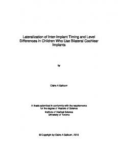


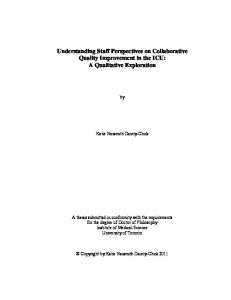


![Thesis - TSpace - University of Toronto [PDF]](https://m.moam.info/img/260x300/thesis-tspace-university-of-toronto-pdf_647daf3c098a9e791c8b459f.jpg)