A comparison between neural network forecasting ... - Semantic Scholar

402

IEEE TRANSACTIONS ON NEURAL NETWORKS, VOL. 10, NO. 2, MARCH 1999

A Comparison Between Neural-Network Forecasting Techniques—Case Study: River Flow Forecasting Amir F. Atiya, Senior Member, IEEE, Suzan M. El-Shoura, Samir I. Shaheen, Member, IEEE, and Mohamed S. El-Sherif

Abstract— Estimating the flows of rivers can have significant economic impact, as this can help in agricultural water management and in protection from water shortages and possible flood damage. The first goal of this paper is to apply neural networks to the problem of forecasting the flow of the River Nile in Egypt. The second goal of the paper is to utilize the time series as a benchmark to compare between several neural-network forecasting methods. We compare between four different methods to preprocess the inputs and outputs, including a novel method proposed here based on the discrete Fourier series. We also compare between three different methods for the multistep ahead forecast problem: the direct method, the recursive method, and the recursive method trained using a backpropagation through time scheme. We also include a theoretical comparison between these three methods. The final comparison is between different methods to perform longer horizon forecast, and that includes ways to partition the problem into the several subproblems of steps ahead. forecasting

K

Index Terms— Backpropagation, Fourier series, multistep ahead prediction, neural networks, Nile River, river flow forecasting, seasonal time series, time series prediction.

I. INTRODUCTION

time series might start to exhibit a gradual and accelerating increase, giving some indication of a start of an upward trend. Another time series can exhibit some past random-like cyclical behavior, and can therefore give a hint about the probable position in the cycle at a certain instant in the future. We present here another neural-network forecasting application, namely river flow forecasting. Forecasting river flows is an important application, that attracted the interest of scientists for more than 50 yrs. It can help in predicting agricultural water supply, predicting potential flood damage, estimating loads on bridges, etc. In this paper the first goal is to apply neural networks to the problem of predicting the flow of the River Nile in Egypt (see [8] for a preliminary application). In addition, we exploit the river forecast problem as a benchmark to compare between different neural network forecasting approaches. The approaches, which all use multilayer networks with backpropagation training, are mainly different approaches to preprocess the time series and different approaches to solve the multistep ahead forecast problem. II. ON

F

ORECASTING the behavior of complex systems has been a broad application domain for neural networks. In particular, applications such as electric load forecasting [1], [2], economic forecasting [3], [4], forecasting natural and physical phenomena [5] have been widely studied, to the extent that now there are several yearly conferences with specific emphasis on the topics of economic forecasting [6], [7]. Forecasting is a highly “noisy” application, because we are typically dealing with systems that receive thousands of inputs, which interact in a complex nonlinear fashion. Usually with a very small subset of inputs or measurements available from the system, the system behavior is to be estimated and extrapolated into the future. What gives some hope to solve some of the difficult forecasting problems is that typically successive events or inputs that affect the time series are serially correlated, and that causes a time series pattern that can give some hint of the future. For example, some economic Manuscript received May 6, 1997; revised December 10, 1998 and January 4, 1999. A. Atiya is with the Department of Electrical Engineering, Caltech, Mail Stop 136-93, Pasadena, CA 91125 USA. S. El-Shoura and M. S. El-Sherif are with the Electronic Research Institute, Tahrir Street, Dokki, Giza, Egypt. S. I. Shaheen is with the Department of Computer Engineering, Faculty of Engineering, Cairo University, Giza, Egypt (e-mail: [email protected]). Publisher Item Identifier S 1045-9227(99)02343-7.

THE

FLOW FORECAST PROBLEM

River flow forecasting is one of the earliest forecasting problems that have attracted the interest of scientists. In fact, Hurst’s work in the 1940’s on the River Nile flow forecast led to the development of the Hurst coefficient [9] (see also [10]), one of the important measurements characterizing the degree of mean reversion of a time series. The importance of estimating river flows to the livelihoods of the inhabitants around rivers made them study and record their levels since earliest history. In fact, there are records for the flow level of the River Nile dating back to around 3000 B.C. (For example, in the Palermo Stone [11], see also [12], the ancient Egyptians recorded the annual peak river levels for the years from 3050 B.C. until 2500 B.C.) This has produced one of the longest recorded time series of a natural phenomenon. It can therefore be of use, not only for studying the river flow problem itself, but also as a benchmark time series for studying and comparing different forecasting algorithms. The problem of flow forecast for the River Nile is particularly important for Egypt. Egypt depends almost exclusively on the Nile for agricultural irrigation. The flow of the River Nile is far from steady, and it exhibits a seasonal behavior. The flow is low during the winter months, and peaks during the months of August and September. The High Dam of Aswan (located South of Egypt) retains incoming water, and releases

1045–9227/99$10.00  1999 IEEE

ATIYA et al.: COMPARISON BETWEEN NN FORECASTING TECHNIQUES

it in a more uniform way, so as to optimally fill agricultural and electricity generating needs (acting like the capacitor or the reservoir effect). Forecasting the flow of the river Nile can help in determining the optimum amount of water to release, and thus can help to more efficiently manage the water. The river flow forecasting problem has been traditionally tackled using linear techniques, such as AR, ARMAX, and Kalman filter, and also using nonlinear regression (see [13]–[17]). We have found only one method in literature that uses neural networks, namely for the Huron River in Michigan [16]. Most of the forecasting methods consider one-day ahead forecast. For the River Nile a longer term forecast such as ten-day ahead or a month ahead is more of interest, though it is more difficult than the one-day ahead problem. These two cases would therefore be the subject of this paper. We used readings of the average daily flow volume for each ten-day period at the Dongola station, located in Northern Sudan (south of the High Dam). The readings spanned the period from 1974 to 1992. We also created from these data a time series of monthly records, by taking the average of the data within each month. We applied our algorithms for these two time series: the ten-day and the monthly time series. III. NEURAL-NETWORK APPLICATION Most neural network approaches to the problem of forecasting use a multilayer network trained using the backpropagation , where it algorithm. Consider a time series is required to forecast the value of . The inputs to the multilayer network are typically chosen as the previous values and the output will be the forecast. The network is trained and tested on sufficiently large training and testing sets, that are extracted from the historical time series. In addition to previous time series values, one can utilize as inputs the values or forecasts of other time series (or external variables) that have a correlated or causal relationship with the series to forecasted. For our river flow problem such time series could be the rainfall at the river’s origins. For the majority of forecasting problems such external inputs are not available or are difficult to obtain. We have not used any external inputs except an input indicating the season. As is the case with many neural-network applications, preprocessing the inputs and the outputs can improve the results significantly. Input and output preprocessing means extracting features from the inputs and transforming the target outputs in a way that makes it easier for the network to extract useful information from the inputs and associate it with the required outputs. Preprocessing is considered an “art,” and there are no set rules to choose it. Even some very intuitively appropriate transformations may turn out of no value when checking the actual results. For our case the main inputs are the previous time series values. We have used some preprocessing of the inputs, but also some of the methods described next section are based also on different ways to preprocess the data. In short, the inputs that we used are combinations of the following: 1) the flows at the previous few time periods; 2) the flow at the same time period 1 yr ago and 2 yr ago;

403

3) the average of the flow of the last 12 months; 4) the period number (scaled by the number of periods), e.g., for the month of May the input would be 5/12. For the ten-day ahead problem we used 150 points for each of the training stage and the testing stage. For the one-month ahead problem, the number of training data and testing data were 100 each. We used as error measurement the normalized root mean square error (NRMSE), defined as follows:

NRMSE

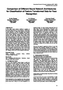
where is the forecast of . We used a network consisting of one hidden layer, with three hidden nodes in the hidden layer, and trained it using the standard backpropagation method. The network is trained for 4000 iterations. We have performed simulations, and found the following observations. 1) There is a strong correlation between the training error and the testing error. This means that there is good generalization. Choosing a network/input set that gives a low training error will almost surely result in a low testing error. 2) In several exploratory runs we have found that no validation set was needed to determine optimal stopping point in training. The error for the test set goes down uniformly with iteration and does not bottom out. 3) For the majority of input combinations the results were somewhat similar. There were several cases which gave higher errors, but these were mostly for cases with insufficient number of inputs, and one can eliminate them easily by observing the training error. 4) The forecasts for all periods of the yr were quite accurate. Only for the peak flow periods there was some small error (see Fig. 1 for the test forecast results of a ten-day ahead case). This suggests possibly training a separate network for the high flow periods, and using some kind of mixtures of experts type network (see [18]–[20]). IV. ALGORITHM COMPARISON In addition to this basic neural-network implementation, we used the data as a benchmark to compare between different neural-network forecasting methods. The methods we used are the following. Method 1: The neural network is trained to forecast the actual flow of the next time period. Method 2: The neural network is trained to forecast the difference in flow between next period’s flow and current period’s flow [the desired output for the neural network at , properly scaled]. time is Method 3: We subtract the seasonal average of the flow to create a seasonally adjusted time series. Then we apply the neural network to forecast this seasonally adjusted series. This approach, hopefully, makes it a simpler problem for the neural network, by letting the neural network concentrate on forecasting the deviations from the seasonal average,

404


Fig. 1. The results of the ten-day ahead forecast for the test period.

rather than estimating both the seasonal average and the deviation. Method 4: A novel algorithm we propose here, that might be particularly suitable for seasonal (cyclical) time series. be the time series values, and let the period (of Let the cycle) be fixed (say ), but however the time series varies from cycle to the other, and can have a longer term yr, because that variation or trend. In our case is the period of the river flow time series. Because of the seasonality of the time series, the Fourier series will be a natural representation of such series, and will carry much useful information relevant to the task of forecasting the series. Therefore, it seems to be potentially an effective method to predict the Fourier coefficients, by giving them as inputs to the neural network. For every time we calculate the discrete , Fourier series (DFS) of the points [the subscript to obtain DFS coefficients in represents the frequency]. These represent the result of a moving window of the DFS calculation. Since the DFS coefficients are complex numbers, we consider the and the imaginary component real component separately. We train a separate neural network for every DFS coefficient and for each of the real and imaginary components. The network takes previous values of the DFS coefficient time series as inputs [that is, for example, for the network corresponding to the real part of the th DFS coefficient], and is trained to estimate the . Once all forecasts from the future coefficient neural networks are available, they are inverted to obtain an estimate for the whole signal in the -long period from to . The estimate of the signal at the end ) is taken as the signal forecast. of the period (at time Fig. 2 shows a block diagram of the method. An analogous approach has been proposed in [21], but with using wavelet transformation, to forecast different resolutions of currency time series.

Fig. 2. A block diagram of the DFS method.

Section VI presents the results of the comparison between these methods. V. THE MULTISTEP AHEAD PROBLEM In addition to these methods, we considered the problem of forecasting several steps away (the multistep ahead problem). , and would like Thus, we have a time series to forecast , where . Of course the larger is, the more difficult the problem is. We have considered several methods to implement the multistep ahead forecast problem, and we will compare between these methods. The methods are as follows. Method 5—Direct Method: We train the neural network to directly forecast the th period ahead. Thus, the desired output . for the network will be Method 6—Recursive Method: We consider a network that forecasts a single step ahead, and apply this network recurstep ahead. Thus, at any intermediate sively to forecast step the network will use some of the forecasts it obtained at previous steps as inputs. There are two basic methods to train such a network. We implemented these two methods in the comparison:


405

Fig. 3. The cascaded architecture for training the recursive implementation of multistep ahead forecasting.

a) To train the network to perform simply a single step ahead forecast. b) To consider a backpropagation through time scheme [22]. That is, we consider the steps ahead forecast as the result of a cascade of identical networks, and train this composite structure of networks (see Fig. 3). Method 6a) is called in the systems identification literature the series-parallel method, and Method 6b) is called the parallel method [23]. Some other approaches for the multistep ahead prediction have also been suggested in literature. For example, [24] has suggested a hybrid approach (between the direct method and the recursive method). However, this method will not be included in the comparison.

Expanding (4) into Taylor series expansion, and retaining up to second-order terms, we get

(5) is the derivative of [the outer as defined in where is its second (2)] with respect to its first argument, and derivative with respect to its first argument. We get

(6) The error obtained for the direct method becomes

A. Theoretical Comparison To gain some theoretical insight into the differences between the direct and the recursive methods, we consider a nonlinear autoregressive system, given by (1)

(7)

is a stationary independent zero-mean process, with where Variance( . For simplicity, let also , means expectation. We will compare between the where recursive method and the direct method under the assumption that we have an unlimited training set, and that the neural network is powerful enough (large enough) to learn any given function accurately. Consider the problem of two step ahead forecast. Generalization to the general multistep ahead problem is straightforward. Consider first the direct method. The value of after two twice] is time steps [i.e., after applying

Expanding into Taylor series and retaining up to fourth powers, we get (8) Now consider the recursive method, trained according to looking one step ahead [Method 6a)]. The objective function in this case will be (9) where the optimal

will be simply (10)

(2) and the expectation of the square of the error

is

The two step ahead error becomes

(3) denotes expectation and represents the neuralwhere network function. The optimal with respect to the expected square error can be shown to be simply the expectation of the , i.e., function

(11) which is evaluated as (12) One can see by comparing between (8) and (12) that

(4)

406


is lower, and therefore the direct method and hence is more superior than the recursive Method 6a). As of the recursive Method 6b), it is trained according to looking two steps ahead [Method 6b)]. Thus, it is required to such that find optimal

(14) is minimized. If a

one month ahead forecast is then the average of the outputs of the three networks. Method 9—Recursive Method: We again consider a network that forecasts a single step ahead, and apply this network recursively for three steps. We average the forecasts obtained in the three steps to obtain the one month ahead forecast. We also implement two training procedures. a) Train the network for a single step ahead forecast. b) Train the network using backpropagation through time scheme to forecast the three next steps [similar to Method 6b)].

can be found such that VI. SIMULATION RESULTS

(15) then this method is as good as the direct method. If such cannot be found, then the direct method is better. We a cannot exist. believe that there are problems where such a The reason is that the “inside ” in the lefthand side of (15) , otherwise there has to be invertible in terms of , could be problems where two different values of all other ’s being the same, should have different right-hand side values, but are stuck with same left-hand side values. The invertibility is a strong requirement, and therefore a that satisfies (15) might not be found. To summarize, the direct method is always better than the recursive Method 6a), and is either better or the same as the recursive Method 6a), depending on the problem considered. Next section gives the experimental comparison results between these three methods. B. Longer Horizon Forecast In addition to the multistep ahead problem, we consider also the problem of forecasting a somewhat long time horizon. This means that we would like to forecast the average flow of the next steps. This problem is somewhat easier than the steps ahead problem, because averaging cancels out some of the error in the forecasts (for example, if we use simply the average yearly flow over the training set as a forecast for the 1 yr ahead flow, the error will not be extremely large). Now comes the question: is it better to partition the problem into different intervals, and forecast each interval separately, or perform a one-shot forecast? The answer to this question is obtained in the comparison. Assume we have a ten-day time series, and we would like to forecast one month ahead (the average of the next three periods). The methods we use are the following. Method 7—Direct Method: We train the neural network to directly forecast the one month ahead. Thus the desired output . for the neural network will be Method 8: We partition the problem to three subproblems: forecast of next step, forecast of two steps away, and forecast of three steps away. We train three neural networks, each to . Thus, for the forecast periods ahead, where periods ahead network, the desired output will be . The

We have performed the comparisons for each of the single step ahead group and the multistep ahead groups. For all runs we used a three hidden node network. We note that the results for all methods did not differ much when varying the number of hidden nodes between 2 and 8. We trained the network for 4000 iterations. This number of iterations was more than enough for adequately training each of the comparison methods. For each comparison we performed five different runs using five different combinations of the inputs described in Section III. We used the following five combinations. Combination 1: The flow at the previous three periods, and the flow at the same period to be forecasted but 1 yr ago. Combination 2: The flow at the previous two periods, the flow at the same period to be forecasted but 1 yr ago, and the period number. Combination 3: The flow at the previous three periods. Combination 4: The flow at the previous six periods. Combination 5: The flow at the previous four periods, the flow at the same period to be forecasted but 1 yr ago, the average flow over the previous 12 months, and the period number. We used the same five input combinations for every method in the comparison, to make the comparison as fair as possible. The only exception is for the discrete Fourier series method (Method 4). Not all the inputs discussed above have a meaning for Method 4, because the discrete Fourier series transformation changes the nature and the meaning of the resulting time series. For this method we used the following five combinations. Combination 6: The previous three values in each DFS coefficient time series. Combination 7: The previous four values in each DFS coefficient time series. Combination 8: The previous three values in each DFS coefficient time series, and the value same period to be forecasted but 1 yr ago. Combination 9: The previous seven values in each DFS coefficient time series. Combination 10: The previous eight values in each DFS coefficient time series. For the multistep ahead and the longer horizon forecast comparisons we used also the input combinations 1–5, except for the recursive Methods 6b) and 9b). For these methods using the average flow of the last 12 months and the period


407

TABLE I (a) TRAINING ERROR FOR THE SINGLE STEP (TEN DAY AHEAD) PROBLEM FOR METHODS 1–4. (b) TESTING ERROR FOR THE SINGLE STEP (TENDAY AHEAD) PROBLEM FOR METHODS 1–4

TABLE II (a) TRAINING ERROR FOR THE TWO STEP AHEAD PROBLEM FOR METHODS 5, 6a), AND 6b). (b) TESTING ERROR FOR THE TWO STEP AHEAD PROBLEM FOR METHODS 5, 6a), AND 6b)

(a)

(a)

(b)

number as inputs will complicate the training algorithm to the extent that it might not learn well and will more possibly get stuck in a local minimum. The input combinations used are the following. Combination 11: The flow at the previous three periods, and the flow at the same period to be forecasted but 1 yr ago. Combination 12: The flow at the previous four periods. Combination 13: The flow at the previous three periods. Combination 14: The flow at the previous six periods. Combination 15: The flow at the previous four periods, the flow at the same period to be forecasted but 1 yr ago. Table I(a) shows the training results for the four methods for the single step ahead (ten day ahead) problem, and Table I(b) shows the results for the testing period. One can see that the most basic method, forecasting the actual flow (Method 1) results in the best forecast accuracy. Following that comes Method 2. Then, we find Methods 3 and 4 at about the same performance in last place. The results were generally consistent across all five runs, meaning that the variation in error among the five runs was small. Testing set performance was not much worse than the training performance, particularly for Methods 1 and 2, indicating reasonable generalization. Method 4’s standing improved, however, for longer horizon forecasting. It obtained a testing period NRMSE of 0.344 for the one month ahead problem, versus 0.284 for the Method 1. For the multistep group, we have performed both a two step ahead comparison and a three step ahead comparison. See Tables II(a) and II(b) for, respectively, the training and testing results for the two step ahead case and Tables III(a) and III(b) for, respectively, the training and the testing results for the three step ahead case. One can see that the direct method

(b) TABLE III (A) TRAINING ERROR FOR THE THREE STEP AHEAD PROBLEM FOR METHODS 5, 6a), AND 6b). (b) TESTING ERROR FOR THE THREE STEP AHEAD PROBLEM FOR METHODS 5, 6a), AND 6b)

(a)

(b)

(Method 5) is superior, especially for the three step ahead case [for the two step ahead it is a tie with the recursive Method 6b)]. The recursive method trained using a backpropagation through time approach was much better than that trained to perform a single step ahead forecast. One can observe that

408


TABLE IV (a) TRAINING ERROR FOR THE ONE MONTH AHEAD PROBLEM FOR METHODS 7, 8, 9a), AND 9b). (b) TESTING ERROR FOR THE ONE MONTH AHEAD PROBLEM FOR METHODS 7, 8, 9a), AND 9b)

(a)

(b)

the experimental results agree with the theoretical comparison performed in Section V-A. We observe that for all methods, input combinations possessing the flow value at the same period to be forecasted but 1 yr ago, resulted in lower error than the combinations possessing purely previous flow values. The reason is that the yr ago flow provides some reference about the approximate level of the flow of the period to be forecasted, because of the cyclicality of the time series. In the last experiment we compared between the longer horizon forecast methods. Assume we would like to forecast one month ahead, in other words the average of the three steps ahead. Tables IV(a) and IV(b) show, respectively, the training results and the testing results. The ranking of the methods in terms of the test results is: Methods 7, 8, 9b), and in last place 9a). One can therefore say that the partitioning of the problem into the subproblems of forecasting the flows at different intervals has not helped. The one shot forecast method has been the best method. We observe also the effect of the yr ago input in improving the results, even for Method 7. VII. CONCLUSIONS The first goal of this paper has been to apply neural networks to the problem of forecasting the flow of the River Nile. We have seen that neural networks produced fairly accurate forecasts. Generalization performance was very reasonable, indicating confidence in the training results as a way to compare different methods and different input combinations. The other goal has been to compare between different methods to preprocess the inputs and the outputs, and different approaches for the multistep ahead problem. Although the

comparative ability of the different approaches is usually problem dependent, this comparison should give some insight, and is therefore an addition to other comparison studies such as [5]. The results of the single step ahead problem yielded a somewhat surprising conclusion. Such intuitive preprocessing as differencing the output, subtracting the seasonal average, or taking the discrete Fourier series, produced worse results (than the most basic method with no preprocessing). Although the DFS method seems intuitive by virtue of the cyclicality of the time series, perhaps the accumulation of the errors of the networks offsets the fact that each network can forecast more accurately. Concerning Method 2, perhaps the differencing accentuates the noise (because it is similar to a differentiation operation), leading to a noisier target output. It would be interesting to know whether these results apply for other forecasting applications. The multistep ahead comparison yielded the direct method as the best method. It also confirmed the fact, well known in the neural-network community, that the backpropagation through time approach is what is needed to train a recursive approach. Concerning the longer horizon forecast, forecasting the whole period in one step tends to work better. It would be interesting to find out how would other architectures such as radial basis functions fare. We feel that the inputs selected and the preprocessing have a bigger weight than the architecture. However, this can be an interesting study to pursue. ACKNOWLEDGMENT The authors would like to acknowledge Dr. A. Parlos of Texas A&M University for a useful suggestion. They would also like to thank Dr. A. Ghanem of Cairo University for supplying the data. REFERENCES [1] J. Connors, D. Martin, and L. Atlas, “Recurrent neural networks and robust time series prediction,” IEEE Trans. Neural Networks, vol. 5, pp. 240–254, Mar. 1994. [2] D. Park, M. El-Sharkawi, R. Marks, L. Atlas, and M. Damborg, “Electric load forecasting using an artificial neural network,” IEEE Trans. Power Syst., vol. 6, pp. 442–449, May 1991. [3] Y. Abu-Mostafa and A. Atiya, “Introduction to financial forecasting,” J. Appl. Intell. [4] A. Refenes and M. Azema-Barac, “Neural network applications in financial asset management,” Neural Comput. Applicat., vol. 2, pp. 13–39, 1994. [5] A. Weigend and N. Gerschenfeld, Eds., Time Series Prediction: Forecasting the Future and Understanding the Past. Reading, MA: Addison-Wesley, 1994. [6] A. Weigend, A. Refenes, and Y. Abu-Mostafa, Eds., in Proc. Neural Networks in the Capital Markets Conf. Pasadena, CA: World Scientific, Nov. 1996. [7] Proc. IEEE/IAFE Conf. Comput. Intell. Financial Eng. New York: IEEE, Mar. 1996. [8] A. Atiya, S. El-Shoura, S. Shaheen, and M. El-Sherif, “River flow forecasting using neural networks,” in World Congr. Neural Networks, San Diego, CA, Sept. 1996, pp. 461–464. [9] H. Hurst, “Long term storage capacity of reservoirs,” Trans. Amer. Soc. Civil Eng., pp. 770–808, 1950. [10] R. Bras and I. Rodriguez-Iturbe, Random Functions and Hydrology. Reading, MA: Addison-Wesley, 1985. [11] The Palermo Stone, 2480 B.C., Palermo Historical Museum, Palermo, Italy. [12] R. Said, The River Nile. Oxford, U.K.: Pergamon, 1993.


[13] H. Awwad, J. Valdes, and P. Restrepo, “Streamflow forecasting for Han River Basin, Korea,” J. Water Resources Planning Management, vol. 120, no. 5, pp. 651–673, 1994. [14] Y. Cheng, “Evaluating an autoregressive model for stream flow forecasting,” in Proc. Hydraulic Eng. Conf., pp. 1105–1109, 1994. [15] D. Burn and E. McBean, “River flow forecasting model for the Sturgeon River,” J. Hydraulic Eng, vol. 111, no. 2, pp. 316–333, Feb. 1985. [16] N. Karunanithi, W. Grenney, D. Whitley, and K. Bovee, “Neural networks for river flow prediction,” J. Computing Civil Eng., vol. 8, no. 2, pp. 203–219, Apr. 1994. [17] M. El-Fandy, Z. Ashour, and S. Taiel, “Time series models adoptable for forecasting Nile floods and Ethiopian rainfalls,” Bull. Amer. Meteorological Soc., vol. 75, no. 1, pp. 1–12, Jan. 1994. [18] R. Jacobs and M. Jordan, “A competitive modular connectionist architecture,” in Advances in Neural Inform. Processing Syst. 3, R. Lippmann, J. Moody, and D. Touretzky, Eds. San Mateo, CA: Morgan Kaufmann, 1991, pp. 767–773. [19] S. Haykin, Neural Networks: A Comprehensive Foundation. New York: IEEE Press, 1994. [20] A. Weigend, M. Mangeas, and A. Srivastava, “Nonlinear gated experts for time series: Discovering regimes and avoiding overfitting,” Int. J. Neural Syst., vol. 6, pp. 373–399, 1995. [21] V. Bjorn, “Optimal multiresolution decomposition in financial time series,” in Proc. Neural Networks Capital Markets Conf., Pasadena, CA, Nov. 1994. [22] P. Werbos, “Backpropagation through time: What it does and how to do it,” Proc. IEEE, vol. 78, Oct. 1990. [23] K. Narendra and K. Parthasarathy, “Identification and control of dynamical systems using neural networks,” Trans. Neural Networks, vol. 1, pp. 4–27, 1990. [24] X. Zhang and J. Hutchinson, “Simple architectures on fast machines: Practical issues in nonlinear time series prediction,” in Time Series Prediction: Forecasting the Future and Understanding the Past, A. Weigend and N. Gerschenfeld, Eds. Reading, MA: Addison-Wesley, 1994, pp. 219–241.

Amir F. Atiya (S’86–M’90–SM’97) was born in Cairo, Egypt, in 1960. He received the B.S. degree in 1982 from Cairo University, Giza, Egypt, and the M.S. and Ph.D. degrees in 1986 and 1991 from California Institute of Technology, Pasadena, all in electrical engineering. From 1985 to 1990, he was a Teaching and Research Assistant at Caltech. From September 1990 to July 1991, he held a Research Associate position at Texas A&M University, College Station. From July 1991 to February 1993, he was a Senior Research Scientist at QANTXX, in Houston, TX, a financial modeling firm. In March 1993, he joined the Computer Engineering Department at Cairo University as an Assistant Professor. He spent the summer of 1993 with Tradelink Inc., Chicago, IL, and the summers of 1994, 1995, and 1996 with Caltech. In March 1997, he joined Caltech as a Visiting Associate in the Department of Electrical Engineering. In January 1998, he joined Simplex Risk Management Inc., Hong Kong, as a Research Scientist, and he is currently holding this position jointly with his position at Caltech. His research interests are in the areas of neural networks, learning theory, theory of forecasting, pattern recognition, data compression, and optimization theory. His most recent interests are the application of learning theory and computational methods to finance. Dr. Atiya received the Egyptian State Prize for Best Research in Science and Engineering in 1994. He also received the Young Investigator Award from the International Neural Network Society in 1996. Currently, he is an Associate Editor for the IEEE TRANSACTIONS ON NEURAL NETWORKS. He served on the organizing and program committees of several conferences, most recent of which is Computational Finance CF99, New York, and IDEAL’98, Hong Kong.

409

Suzan M. El-Shoura received the B.S. degree in electronics and communications engineering with honors from Cairo University, Giza, Egypt, in 1992 and the M.S. degree in computer engineering from Cairo University, in 1997. She is a Research Assistant in the Department of Computers and Systems at Electronics Research Institute (ERI), Giza, Egypt. Her research interests include neural networks and its applications in forecasting.

Samir I. Shaheen (S’74–M’81) received the B.Sc. and M.Sc. degrees from the Department of Electronic and Communication Engineering at Cairo University, Giza, Egypt, in 1971 and 1974, and the Ph.D. degree from McGill University, Montreal, Canada, in 1979. From 1979 to 1981, he worked in the Computer Vision Lab of McGill University. In 1981, he joined Cairo University as an Assistant Professor. He joined the Computer Science Department, King Abdulaziz University, Saudi Arabia, as a Visiting Professor. He is currently a Professor in the Computer Engineering Department, Cairo University, and the Director of the Computer Labortatories. He is the manager of Cairo University Computer Network and Computer Research Center. His current research interests include neural networks, medical imaging, document analysis, and multimedia in high-speed digital networks.

Mohamed S. El-Sherif received the B.S. and M.S. degrees in electronics and communications engineering from Cairo University, Giza, Egypt, in 1974 and 1978, respectively. He received the Ph.D. degree jointly from Cairo University and Ohio State University, Columbus, in 1981. Since then, he has been with the Electronics Research Institute (ERI), Giza, Egypt. Currently, he is the head of the Computer Engineering Department at ERI.