A Comparison of Bayesian Methods and Artificial Neural Networks for ...

J. Stat. Appl. Pro. 1 No. 2, 89-100 (2012)

89

Journal of Statistics Applications & Probability An International Journal © 2012 NSP

@ 2012 NSP Natural Sciences Publishing Cor.

A Comparison of Bayesian Methods and Artificial Neural Networks for Forecasting Chaotic Financial Time Series Tamer Shahwan1 and Raed Said2 1

Al Ain University of Science and Technology, College of Business Administration, Department of Accounting, Finance & Banking, P.O. Box: 64141, Al Ain, United Arab Emirates.

Email Address: [email protected] 2

Al Ain University of Science and Technology, College of Business Administration, Department of Management Information Systems, P.O. Box: 64141, Al Ain, United Arab Emirates.

Email Address: [email protected] Received March 16, 2012; Revised April 20, 2012; Accepted April 25, 2012

Abstract: Most recent empirical work implies that the presence of low-dimensional deterministic chaos increases the complexity of the financial time series behavior. In this study we propose the Generalized Multilayer Perceptron (GMLP), and the Bayesian inference via Markov Chain Monte Carlo (MCMC) method for parameter estimation and one-step-ahead prediction. By out-of-sample prediction approach, these proposed methods are compared to autoregressive integrated moving average (ARIMA) models which have been used as a benchmark. The deterministic Mackey-Glass equation with errors that follow an ARCH (p) process (MG-ARCH (p)) is applied to generate the data set used in this study. It turns out that GMLP outperforms the other two forecasting methods using RMSE, MAPE, and MAE criteria of forecasting accuracy. Keywords: ARIMA; Artificial Neural Networks (ANNs); Bayesian inference; MG-ARCH (p) model; one-step-ahead forecasting

1 Introduction Obtaining accurate stock prices forecast is one of the main goals of financial and academic research institutions which they seek to achieve for the purpose of supporting key financial decisions such as selling and hedging. However, accurate forecasting of stock prices remains a major challenge under efficient market conditions (Shahwan, 2006). Much effort has been devoted over the past decades to the development of time series forecasting models. Traditionally, Autoregressive integrated moving average (ARIMA) models are considered as some of the most widely used linear models in time series forecasting because of their theoretical elaborateness and accuracy in shortterm forecasting (Jhee and Shaw, 1996). However, ARIMA models cannot easily capture non-linear patterns resulting from the existence of a bounded rationality assumption in financial markets (McNelis, 2005). In recent years, however, interest in the use of artificial neural networks (ANNs) for forecasting and time series prediction has grown steadily (Zhang et al. 1998) as has interests in the applications of Bayesian inference in forecasting time series (Mendoza and De Alba, 2006). In this paper, we will examine the ability of Bayesian inference via Markov Chain Monte Carlo (MCMC) method for forecasting time series using simulation data. MCMC is a sampling based

90

Tamer Shahwan, et al.: A Comparison of Bayesian Methods and Artificial .....

simulation technique that generates a dependent sample from a certain distribution of interest. Several schemes of implementing MCMC methods are widely used in Bayesian inference such as the Gibbs sampler introduced by (Geman and Geman, 1984) and Metropolis-Hasting method originally developed by (Metropolis et al. 1953) and further generalized by (Hastings, 1970). These two algorithms are simple to implement and are effective in practice when used for Bayesian inference (Surapaitoolkorn, 2007). The stochastic Mackey-Glass process is generated using Monte Carlo experiment since the chaotic time series has a lot of similarity to economic and financial time series (McNelis, 2005). In this paper we compare Bayesian estimation methods with artificial neural networks. ARIMA models will be used as a benchmark. The comparability or superiority of the proposed models will be investigated using Monte Carlo experiments. The main motivation of this approach is due to the existence of little empirical evidence regarding the performance of ANN, Bayesian estimation methods and ARIMA models under different characteristics of chaotic financial time series. Therefore, using a simulation study which covers a wide range of these characteristics will enable us to identify the conditions under which one of these models is superior to others. The remaining part of the paper is organized as follows. Section 2 describes different proposed forecasting methods employed for time series forecasting. The numerical simulation in section 3 includes generation of the data using Mackey-Glass stochastic process, specification of the forecasting models and performance measures. The results are presented in section 4. Finally, section 5 gives concluding remarks and some suggestions for future work. 2 Forecasting Methods 2.1 ARIMA Models Consider the following stochastic process yt , t  N  that can be expressed in terms of its conditional moments as follows (Campbell et al. 1997, p. 469) and (Shahwan, 2006, p. 8): yt  g Ft 1   hFt 1    t

(1)

where  t  at  t is a standardized shock. a t is a white noise series with a mean of zero and a

variance  t2 , Ft 1 is the collection of yt 1 , yt 2 ,...., yt  p  and at 1 , at 2 , , at a  , g  represents a linear or nonlinear function, and h   t2 . Accordingly, the stochastic process of the time series y t will be a non-linear in mean if the g  is a non-linear function, whereas a time series with non-linear h is said to be non-linear in variance. A linear autoregressive moving average (ARMA) model of order  p, q  implies that the current value of y t of the process can be expressed as a linear combination of its past values yt 1 , yt 2 ,...., yt  p  and a random shock series at 1 , at 2 ,, at a  . Thus, the ARMA model can be expressed as follows (Tsay, 2005): p

q

i 1

i 1

y t   0    i y t i   i a t i

(2)

where  ,    0 ,....,  p , 1 ,....,  q  are the parameters of the model. p and q are non negative integers. Since many time series are non-stationary, differencing one or more times is required. This leads to the well-known autoregressive integrated moving average (ARIMA) model. By using the back shift operator  with  yt   yt 1 , ARIMA model can then be written as follows (Pindyck and


91

Rubinfeld, 1991):

1       1

2

2







    p  p 1   y t  1  1   2  2     q  q at , d

with 1   2     p  1

(3)

where d is the level of differences used to change non-stationary time series into stationary time series. Basically, the fitting of ARIMA  p, d , q  model to a given time series consists of the following three phases: (i) Model identification, by analyzing the behavior of the autocorrelation function (ACF) and the partial autocorrelation function (PACF), aims to determine the proper orders of  p, q  , (ii) Parameters estimation by using the maximum likelihood technique, and (iii) Forecasting of new values based on the estimated parameters. It is worthwhile to mention that ARIMA models cannot capture non-linear patterns in time series data. In the following section, we examine artificial neural networks, as a non-parametric data-driven approach with the capability of capturing nonlinear patterns that expected to be existed in the data of volatile financial markets. 2.2 Artificial Neural Networks (ANNs) The artificial neural networks (ANNs), as representative of a more general class of non-linear models, are probably one of the most frequently used tools in finance and economics. Well-known applications of this model include credit approval, bankruptcy prediction, and time series prediction [See Jensen (1992); Raghupathi et al. (1996) and Tam and Kiang (1996)]. With regard to one-stepahead prediction yˆt 1 , artificial neural networks determine the function  f  using the historical observations  yt , yt 1 ,...., yt n  with n  1,....., N  denoting the number of input units as follows (Shahwan, 2006):

yˆ t 1  f  yt , yt 1 ,, yt n 

(4)

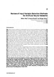
An ANN model is defined in terms of subsidiary decisions such as selecting the architecture of the artificial neural networks, determining the number of hidden layers, the number of hidden neurons, the number of input nodes in the input layer, the type of activation function, the values of the learning rate and the way the data is to be divided into training, cross validation, and test sets (Shahwan, 2006). Based on Occam's razor principle, the simpler network will be selected to strike a balance between training performance and network complexity (Azoff, 1994). A more detailed review of guidelines, rules, and their implications to the ANN output when specifying the optimal ANN is provided by Azoff (1994); Zhang et al. (1998); and Shahwan (2006). In the current study, the Multilayer feedforward with jump connections will be used to conduct one-step-ahead forecasting. This type of neural networks can be considered as a generalization of the MLP (GMLP). Fig. 1 depicts the idea of GMLP where each input node in the input layer is directly connected to the output layer. The GMLP with a "tanh sigmoidal activation function" in the hidden layer and an "identity transfer function" in the output layer has the following structure (Tsay, 2005): I

n k , t  wk , 0   wk , i x i , t

(5)

i 1

M k ,t  f nk ,t  

n

e k ,t  e k ,t n n e k ,t  e k ,t n

(6)

92


k*

I

k 1

i 1

y t   0    k M k ,t   v i xi ,t

(7)

where xi , t , i  1,2,, I , are input variables. w k ,0 and  0 are constants terms, wk ,i are the synaptic weights of input variables and nk ,t is a linear combination of these input variables observed at time

t , t  1,2,, T . Hence, the nk ,t is squashed by the tanh sigmoid activation function and becomes M k ,t at time t . Note that a set of k * neurons k  can be found in the hidden and output layers,  k

denotes the coefficient vector between the hidden and output layer, and vi is the coefficient vector between the input and output layer. Thus, a feedforward network jump connection with a linear function in the output layer can be considered as a generalization of the linear regression model with non-linear terms (Shahwan, 2006). Consequently, if the underlying function between the input and the output is a pure linear, the coefficient sets  and w will be zero, yielding a linear model [see Gonzalez (2000), Tsay (2005) and McNelis (2005)].

Fig. 1. Feedforward network with jump connection (Shahwan, 2006, p.23).

2.3 Markov Chain Monte Carlo (MCMC) Method As an alternative to the classical ARIMA models, it is possible to apply Bayesian inference. De Alba and Mendoza (2007) proved that Bayesian procedures can be more effective, if only a small amount of past data is available, than the classical ARIMA models. It is also preferred to use it in the presence of cycles and trends in the time series data. In this section, we describe how to carry out Bayesian inference for the simulated data using a Gibbs sampling method. Following Koop (2003), Gibbs sampling for independent Normal-Gamma prior is implemented to obtain the Bayesian estimates. As mentioned in section (2.1), an autoregressive model of order p , AR  p  as a linear combination of its p past values is defined as follows: yt  0  1 yt 1  2 yt  2     p yt  p  at

(8)


93

where  0 , 1 ,....,  p  are the parameters of AR  p  model. The Bayesian approach to the parameters estimation of a stochastic process starts by determining the likelihood function p( y /  ) where y  ( y1 , y 2 ,, y N ) is the observed time series and   ( , h)  (0 , 1,,  p , h) is the vector of unknown parameters. 1

1

p ( y /  , h) 

v

h hv {h 2 exp[  (   ˆ )' X ' X (   ˆ )]}{h 2 exp[  2 ]} 2 2s

N

(2 ) 2

(9)

 y p 1   y    , ˆ  ( X ' X ) 1 X ' y , s 2  ( y  Xˆ )' ( y  Xˆ ) v , v  N  p , and y   p  2  .        y N  p   yN 

 yp  y  Where X   p 1     y N 1 

y1 y2 

The estimates of the parameters h and  are performed by MCMC method via Gibbs sampling technique. The form of the above likelihood suggests that the natural conjugate prior is an independent Normal-Gamma. In particular, we assume p( , h)  p( ). p(h) with p(  ) being Normal and p(h) being Gamma: 1

p(  ) 

(2 ) 1 G

p ( h)  c h

p 2

v2 2

V



1 2

exp(

1 1 exp[  (    )'V (    )] 2

(10)

hv ) 2 2s

(11)

where s 2 and v are the prior mean and degrees of freedom of h ,   E ( / y) is the prior mean of

 , and cG is the integrating constant for the Gamma probability density function. Bayes’ theorem allows us to combine the likelihood function with the prior in order to form the conditional distribution of h and  given the observed data y , that is, 1 1 p(  , h / y)  {exp[ {h( y  X ) ' ( y  X )  (    )'V (    )}]}.h 2

N v  2 2

exp[

hv ] 2 2s

(12)

The aim of MCMC simulation is to generate a sample {( j )  (( j ) , h( j ) ), j  1,2,, m} from the conditional densities p(h /  , y) and p( / h, y) obtained from the joint posterior density p( , h / y) . This sample is then used to infer the point estimates of the parameters  and h . For instance, the Bayesian point estimates ˆ and hˆ are given by:

ˆ 

1 m   j m j 1

and

1 m hˆ   h j  m j 1

(13)

As mentioned above, we will use Gibbs sampler as a simulation strategy in our study. One of the main advantages of this sampler is that it is often easier to implement than any of the other MCMC methods. The Gibbs sampler is also flexible in the sense that its output may be used in order to make a variety of posterior and predictive inferences. Following (Geman and Geman, 1984), The Gibbs-Sampler algorithm is briefly described in the following steps:

94


Step (1) Assign initial values to the parameters:  ( 0 ) and h( 0) ; Step (2) Obtain a new observation  ( j 1) from the conditional density p( / h( j ) , y) ; Step (3) Obtain a new observation h( j 1) from the conditional density p(h / ( j 1) , y) ; Step (4) Stop if the convergence of the Markov chains has been detected. Otherwise, do j  j  1 and return to step 2. After a sufficiently large number of iterations, the set of observations (  ( j ) , h( j ) ) converges and it can be treated as a sample from the joint posterior density p( , h / y) . 3 Numerical Simulation and Model Specification Methods In the current simulation experiment, we aim to simulate the price behavior of financial time series using the stochastic Mackey-Glass process. The Mackey-Glass equation was originally developed for modeling white blood cells production (Calvo and Jabri, 2000). The prime motive in selecting this stochastic process is that real economical dynamics is a mixture of deterministic and stochastic chaos (Holyst et al. 2001). Following Kyrtsou and Terraza (2003), the discrete version of the deterministic Mackey-Glass equation is:

rt  d

rt   rt 1 1  rtc

(14)

where rt is the return of the time series. We must note that the choice of lags c and  are vital in determining the dimensionality of the system. In finance, asset return volatility exhibits volatility clustering in the sense that periods of high volatility tend to be followed by high volatility and periods of low volatility tend to be followed by low volatility (Poon, 2005, p. 7). Hence, the basic assumption of the current simulation is that the conditional variance of the stochastic Mackey-Glass process follows an autoregressive conditional heteroscedastic process of order one, ARCH (1). A time discretized realization of that process is:

yt  yt 1  e rt rt  d

rt   rt 1  at 1  rtc

(15) (16)

at   t   t

(17)

 t2   0  1  at21

(18)

where y t denotes the price at time t .  0 is constant,  is the volatility,  1 is the weight assigned to at21 , and  t is a random sample drawn from a standardized normal distribution with mean zero and a standard deviation of one. The set of parameters used to generate the aforementioned stochastic process are y0 12.5 as an initial price. Another important parameter that must be determined is the volatility  . Following Shahwan (2006), the estimated volatility of hog prices in the German spot market is about 14.60%. Accordingly,  02 is set to be 0.0225 as an initial variance. Each value of   1 , c  2 , d  2.1 ,

  0.05 ,  0  0.2 , and 1  0.5 are derived from Kurtsou and Terraza (2003, p. 261).


95

The sample size for the generated data consists of 500 observations. The forecasting performance of the proposed model is assessed by an out-of-sample technique. Each time series is divided into 450 observations as a training set and 50 observations for testing. The training set is used for model specification and then the testing set is used to evaluate the established model. Three criteria are used to evaluate the accuracy of each model. The root mean square error (RMSE), Mean absolute percentage error (MAPE) and Mean absolute error (MAE) are employed to measure the forecasting error. These statistical measures of out-of-sample predictions are: 1 T

RMSE 

MAPE 

MAE 

2

T

  yˆt  yt 

(19)

t 1

100 T yˆ t  yt  y T t 1 t

1 T

T

 yˆ t 1

t

(20)

 yt

(21)

where y t and yˆ t are the actual and the predicted price, respectively, at time t . T is the number of observations in the test set. The Structure of ARIMA model is determined through the following steps: (i) a natural logarithm is applied to each value of y t as an attempt to stabilize the data set. (ii) Investigation of the time series stationarity by applying the augmented-Dickey Fuller test (ADF). ADF statistics is (0.543) and lies inside the acceptance region at 5% level of significance. Therefore, we can not reject the presence of unit root which indicates the non-stationary of the time series. Therefore, the first order difference is applied. (iii) Analyzing the Autocorrelation (ACF) and the partial autocorrelation (PACF) for the time series as shown in fig. (2), each of p and q can be inferred. The best estimated ARIMA model for the data set has the structure 1,1,2 . Without prejudging the nature of nonlinearity existed in our data set, the residuals of ARIMA model have been tested for the presence of nonlinearity using the BDS test1. Following Kanzler (1999, p. 33), the dimensional distance of 1.5 has been selected to yield a better approximation as shown in Table (1). These results indicate that there is a non-linear structure in our data set. The significant evidence of nonlinearity implies that the use of nonlinear model such as ANN might be accurate in fitting the time series. Additionally, we test for the presence of GARCH effects using Engle's ARCH test and Ljung-Box Q-statistic. The results in Table (2) indicate that such effect exist in the data. Hence, the time series is nonlinear in terms of variance.

Estim ated Autocorrelations for Col_1 Au to co rre la tion s

1 0.6 0.2 -0.2 -0.6 -1 0

5

10

15

lag

1

The BDS test examines for (iid) versus general nonlinearity in the time series.

20

25

96


(a)

P art ial Aut ocor relations

Estimated Partial Autocorrelations for Col_1 1 0.6 0.2 -0.2 -0.6 -1 0

5

10

15

20

25

lag

(b) Fig. 2. ACF (a) and PACF (b) for the time series Table 1. The BDS test on the residuals of ARIMA model for the Mackey-Glass series. Dimensional distance of 1.5

Embedding dimension (m) 2

3

4

5

8.4377*

9.3745*

9.5924*

9.3857*

*

indicates the rejection of null hypothesis of (i.i.d) at the 5 % significance level

Table 2. The Ljung-Box Q statistic and Engle's ARCH test for the Mackey-Glass series. Test

Lags Q(5)

The Ljung-Box Q statistics on the residual of ARIMA

*

2.35 *

The Ljung-Box Q statistics on the squared residual of ARIMA

92.34

Engle's ARCH test

70.13*

Q(10)

Q(15)

Q(20)

13.38

18.92

25.03

129.3

*

80.15*

*

137.3*

84.47*

86.77*

131.7

indicates statistical significance for the presence of GARCH effects at the 5% level

The specification of ANN model is now in turn, the generalized MLP network used has six inputs, one hidden layer and one output unit. A genetic algorithm is used to optimize numbers of the hidden nodes, the value of the learning rate, the momentum term and the weight decay constant. The hyperbolic tangent function is chosen as a transfer function between the input and the hidden layer. The identity transfer function connects the hidden with the output layer. The GMLP is trained by back propagation algorithm. To avoid the memorization problem "overfitting" during the training process of ANN model, a cross-validation approach will be applied. 20% of the training set (90 observations) had to be used for cross-validation in the back-propagation approach. Haykin (1999), Principe et al. (2000) and Shahwan (2006) illustrate that the use of cross-validation approach enhances the generalization capability of the neural network model. Batch updating is chosen as the sequence in which the patterns are presented to the network. To set up MCMC methods, the actual observations of the time series y t are transformed by applying a logarithmic transformation. Then, the transformed time series Z t is normalized as


97

follows: log yt  

Zt 

(22)



where  and  are the sample mean and standard deviation of the generated time series. The sample mean and variance of our data are (-4.9433) and (0.071692), respectively. We allowed the MCMC simulation to run S0  1000 iterations in order to burn-in the Gibbs sampler and remove the effect of the starting values of  , i.e., 0  (1,4,4.5) , and then allowed it to run for an additional S1  9000 iterations in order to generate a random sample from the posterior distribution. We set the initial draw for the error prediction to be equal to the inverse of OLS prediction estimate of  2 , i.e., 2 h0  1 S 2  1 0.07692  194 . To see whether the estimated results using MCMC methods are reliable or not we obtain what we call as MCMC diagnostics. Geweke (1992) suggested a convergence diagnostic (CD) given by; CD 

gˆ S A  gˆ S C ˆ A ˆ  C SA SC

(23)

where S A and S C are the set of first and the last draws, respectively. Following Koop (2003), it has been found that setting S A  0.1S1 , and S C  0.4S1 works well in many forecasting application. Let gˆ S A and gˆ SC be the estimate of E ( g ( ) / y) using the first S A replications after the burn-in and the

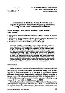
last S C replications, respectively. ˆ A S A and ˆ C S C are the numerical standard errors of CD estimates. The convergence of MCMC algorithm has occurred as CD is less than 1.96 in absolute value for all  0 , 1 ,  3 . Fig. (3) shows the histogram of the samples generated via MCMC simulation using the Normal Gamma prior density. Predictive Density 1400

1200

1000

800

600

400

200

0 -10

-9

-8

-7

-6 -5 -4 Monthly Price

-3

-2

-1

0

Fig. 3. The predictive density for MG- ARCH (1) series

4 Results ARIMA model is estimated with the help of Statgraphics Plus software. The software package NeuroSolutions V5.05 was employed for the estimation of the Generalized Multilayer Perceptron (GMLP). The Bayesian estimates using the Normal-Gamma prior via the Gibbs-Sampling algorithm were carried by Koop's Matlab code which was slightly improved to be popular with our data set. We compare the accuracy of the proposed Bayesian method for forecasting time series with GMLP and ARIMA models using the out-of-sample approach. Table (3) shows the comparison of forecasting errors using different criteria for the proposed methods of our MG-GARCH (1) series. The accuracy criteria of RMSE, MAPE, and MAE shown in table (3) indicate that the GMLP method outperforms the other two methods in one-step-ahead forecasting. Based on Morgan-

98


Granger-Newbold test, the difference in prediction errors of the three different forecasting methods are statistically significant at the 5% level. These results are with our expectation that GMLP will dominate the linear models when the stochastic process of our data set follows a more complex and nonlinear patterns. It is also remarkable to note that the estimated ARIMA 1,1,2 model dominates the MCMC according to the above mentioned accuracy criteria. Our findings are compatible with the results of De Alba and Mendoza (2007) that standard forecasting procedures, like ARIMA, models will yield better forecasting than our proposed Bayesian method for lengthy time series. Table 3. Forecasting errors of ARIMA, GMLP, and Bayesian methods for MG-ARCH (1) series Methods

RMSE

MAPE

MAE

Rank

ARIMA

0.1146

0.5522

0.0839

2

GMLP residuals Bayesian of ARIMA

0.0981*

0.4994*

0.0773*

1

0.6193

3.1812

0.4854

3

*indicates statistical significance in the forecasting accuracy at the 5 % level Bold letter indicates minimal error

5 Conclusions This study has compared the Bayesian inference with artificial neural networks (ANNs) methods in forecasting chaotic financial time series. It has also applied traditional ARIMA models as a benchmark. The findings imply that ANNs are more relevant to fit a high-dimensional chaotic process than the Bayesian and ARIMA methods. However, ANNs demand a lot of specification procedure in determining its optimal structure. It is a time consuming model compared to ARIMA. Unfortunately, there is no fixed method for specifying of ANNs' parameters. The selection almost depends on heuristics. The study also confirms that there is no improvement in the forecast accuracy gained by using the MCMC method. Therefore, it is recommended to extend the MCMC model adopted in this study by using other prior distributions, and different MCMC algorithms. Moreover, there is a need to investigate the accuracy of these forecasting methods; MCMC; ANNs; ARIMA; using different simulated data as well as real data sets. Acknowledgment We gratefully acknowledge financial support from Al Ain University of Science and Technology. We also thank conference participants at the Fourth International conference on Mathematical Sciences ICM 2012- hold in United Arab Emirates University for helpful comments and advice. References [1] E. M. Azoff, Neural Network Time Series Forecasting of Financial Markets. John Wiley & Sons Ltd, Chichester, England, (1994). [2] J. M. Bernardo, A. F. M. Smith, Bayesian Theory. John Wiley and Sons, Ltd., Chichester, (1994). [3] R. Calvo, M. Jabri, Benchmarking Bayesian Neural Networks for Time Series Forecasting, (2000). URL: http://www.cs.cmu.edu, 17.10.2011. [4] J. Y. Campbell, A. W. Lo, A. C. Mackinlay, The Econometrics of Financial Markets. Princeton University Press, Princeton, New Jersey, (1997). [5] G. Casella, E.I. George, Explaining the Gibbs Sampler. The American Statistician, 46 (1992) 167-174.


99

[6] E. De Alba, M. Mendoza, Bayesian Forecasting Methods for Short Time Series. The International Journal of Applied Forecasting, 8 (2007) 41-44. [7] A. K. Dixit, R. S. Pindyck, Investment under Uncertainty. Princeton University Press, Princeton, New Jersey, (1994). [8] A. E. Gelfand, A. F. M. Smith, Sampling Based Approaches to Calculating Marginal Densities. Journal of the American Statistical Association, 85 (1990) 398-409. [9] S. Geman, D. Geman, Stochastic Relaxation, Gibbs Distributions, and the Bayesian Restoration of Images. IEEE Transactions on Pattern Analysis and Machine Intelligence, 6 (1984) 721-741. [10] J. Geweke, Evaluating the Accuracy of Sampling- Based Approaches to the Calculation of Posterior Moments. In J. Bernardo, A. Dawid, A. Smith (Eds.), Bayesian Statistics. Oxford, Clarendon Press, 4th edition, (1992), 641- 649. [11] S. Gonzalez, Neural Networks for Macroeconomic Forecasting: A Complementary Approach to Linear Regression Models. Working paper, Department of Finance Canada, Canada, (2000). URL: http://www.fin.gc.ca/access/wpliste.html, 06.2.2012. [12] W. K. Hastings, Monte Carlo Sampling Methods Using Markov Chains and Their Applications. Biometrika, 57 (1970) 97-109. [13] S. Haykin, Neural Network: A Comprehensive Foundation. Second Edition, Prentice-Hall Inc., New Jersey, (1999). [14] J. A. Holyst, M. Zebrowska, K. Urbanowicz, Observations of Deterministic Chaos in Financial Time Series by Recurrence Plots, Can One Control Chaotic Economy? The European Physical Journal B, 20 (2001) 531-535. [15] H. L. Jensen, Using Neural Networks for Credit Scoring. Managerial finance, 18 (1992) 15-26. [16] W. C. Jhee, M. J. Shaw, Time Series Prediction Using Minimally Structured Neural Networks: An Empirical Test. In R. R. Trippi, E. Turban, (Eds.), Neural Networks in Finance and Investing. Revised Edition, Irwin, Chicago, (1996). [17] L. Kanzler, Very Fast and Correctly Sized Estimation of the BDS Statistics. Working paper, Department of Economics, University of Oxford, Christ church, UK, (1999). [18] G. Koop, Bayesian Econometrics. John Wiley and Sons Ltd, England, (2003). [19] C. Kyrtsou, M. Terraza, Is It Possible to Study Chaotic and ARCH Behaviour Jointly? Application of a Noisy Mackey-Glass Equation with Heteroskedastic Errors to the Paris Stock Exchange Returns Series. Computational Economics, 21 (2003) 257-276. [20] P. D. McNelis, Neural Networks in Finance: Gaining Predictive Edge in the Market. Elsevier Academic Press, (2005). [21] M. Mendoza, E. De Alba, Forecasting an Accumulated Series Based on Partial Accumulation II: A New Bayesian Method for Short Time Series with Stable Seasonal Patterns. International Journal of Forecasting, 22 (2006) 781-798. [22] N. Metropolis, A. W. Rosenbluth, M. N. Rosenbluth, A. H. Teller, E. Teller, Equation of State Calculations by Fast Computing Machines. Journal of Chemical Physics, 21 (1953) 1087-1092. [23] R. S. Pindyck, D. L. Rubinfeld, Econometric Models and Economic Forecasts. McGraw-Hill, Inc., New York, USA, (1991). [24] S.-H. Poon, A Practical Guide to Forecasting Financial Market Volatility. John Wiley & Sons, Ltd., New York, (2005). [25] J. C. Principe, N. R. Euliano, W. C. Lefebvre, Neural and Adaptive Systems: Fundamentals through Simulations. John Wiley & Sons, Inc., (2000). [26] W. Raghupathi, L. L. Schkade, B. S. Raju, A Neural Network Approach to Bankruptcy Prediction. In R. R. Trippi, E. Turban (Eds.), Neural Networks in Finance and Investing. Revised Edition, Irwin, Chicago, (1996). [27] T. Shahwan, Forecasting Commodity Prices Using Artificial Neural Networks. PhD Thesis, HumboldtUniversität Zu Berlin, Berlin, Germany, (2006).

100


[28] W. Surapaitoolkorn, Bayesian Markov Chain Monte Carlo (MCMC) for Stochastic Volatility Model Using FX data. 7th Annual Hawaii International Conference on Business, Honolulu, USA, (2007). [29] K. Tam, M. Kiang, Predicting Bank Failures: A Neural Network Approach. In R. R. Trippi, E. Turban (Eds.), Neural Networks in Finance and Investing. Revised Edition, Irwin, Chicago, (1996). [30] R. S. Tsay, Analysis of Financial Time Series. John Wiley and Sons, Inc., New Jersey, (2005). [31] G. Zhang, B. E. Patuwo, M. Y. Hu, Forecasting with Artificial Neural Networks: The State of the Art. International Journal of Forecasting, 14 (1998) 35-62.