SPKM : A Novel Graph Drawing based Algorithm for Application Mapping onto Coarse-Grained Reconfigurable Architectures Jonghee W. Yoon, †Aviral Shrivastava, Sanghyun Park, Minwook Ahn, †Reiley Jeyapaul, and Yunheung Paek Seoul National University, Korea †Arizona State University, USA {jhyoon, shpark, mwahn}@optimizer.snu.ac.kr †{Aviral.Shrivastava, Reiley}@asu.edu
[email protected]
Abstract— Recently coarse-grained reconfigurable architectures (CGRAs) have drawn increasing attention due to their efficiency and flexibility. While many CGRAs have demonstrated impressive performance improvements, the effectiveness of CGRA platforms ultimately hinges on the compiler. Existing CGRA compilers do not model the details of the CGRA architecture, due to which they are, i) unable to map applications, even though a mapping exists, and ii) use too many PEs to map an application. In this paper, we model several CGRA details in our compiler and develop a graph mapping based approach (SPKM) for mapping applications onto CGRAs. On randomly generated graphs our technique can map on average 4.5X more applications than the previous approaches, while using fewer CGRA rows 62% times, without any penalty in mapping time. We observe similar results on a suite of benchmarks collected from Livermore Loops, Multimedia and DSPStone benchmarks.
I. I NTRODUCTION Coarse Grain Reconfigurable Arrays (CGRAs) have emerged as a promising reconfigurable platform, by providing operation level programmability, word level datapaths, and powerful and very areaefficient datapath routing switches. CGRAs are essentially a set of processing elements (PEs), such as ALUs or multipliers. The PEs are connected so that they can use the result of its neighboring PEs. It is the PE function selection and data routing that provides CGRAs with the reconfigurability. CGRAs can fully exploit the parallelism in an application, and therefore they are extremely well suited for applications that need high throughput including multimedia, signal processing, networking, and other scientific applications. Several CGRA implementations like MorphoSys, RSPA, KressArray, etc. have been proposed. Comprehensive summary of CGRAs can be found in [5]. However, the success of CGRAs critically hinges on the efficient mapping of applications onto it so as to exploit the parallelism in the application and utilize minimum computation resources of the CGRA. Minimizing the number of computation resources in CGRAs is an extremely important goal, as it directly translates into either reduced power consumption, or increased throughput. The problem of mapping an application onto a CGRA to minimize the number of resources used has been shown to be NP-complete, and therefore several heuristics have been proposed. However existing heuristics do not consider the details of the CGRA architecture such as the followings. PE Interconnection Most existing CGRA compilers assume that the PEs in the CGRA are connected only in a simple 2-D mesh fashion, i.e., a PE is connected to it’s neighbors only. However, in most existing CGRAs each PE is connected to more PEs than just the neighbors. In Morphosys, a PE is connected to every other PEs through shared buses, and each PE is connected to the immediate neighbors and the next neighbors also in RSPA. Shared Resources Most CGRA compilers assume that all PEs are similar in the sense that an operation can be mapped
to any PE. However, modern CGRAs, in order to reduce the cost, power and complexity, do not include the multiplier in each PE. Few multipliers are made available as shared resources in each row. For example, RSPA has 2 shared multipliers in each row. Routing PE Most CGRA compilers cannot use a PE just for routing. This implies that in a 4x4 CGRA, it is not possible to map application DAGs in which any node has more than 4 degrees. However, most CGRAs allow a PE to be used for routing only, which makes it possible to map any degree DAGs onto the CGRA. Owing to the simplistic model of CGRA architecture in the compiler, existing CGRA compilers are i) unable to map an application on the CGRA, even though it is possible to map them. ii) uses too many PEs in their solution. The contributions of this paper are: • We formulate the application mapping problem onto CGRA considering the routing PEs, the shared resource constraints and complex PE interconnection. • We develop an integer linear programming (ILP) solution to obtain the optimal application mapping and to compare with our heuristic approach. • We propose a graph drawing based approach to map applications onto CGRAs which can map 4.5X more randomly generated application DAGs than previous approach, while using less rows 62% of time, without any mapping time penalty. The rest of the paper is organized as follows: Section II and Section III formally define the problem of mapping applications onto CGRAs. Section IV describes CGRAs and the previously proposed heuristics for mapping applications onto CGRAs. In Section V, we formulate the application mapping problem with ILP to find the optimal solution, and Section VI proposes our graph drawing based solution. We explain our experimental setup in Section VII and conclude this paper in Section VIII. II. N OTATION AND D EFINITIONS Since applications spend most of their time and power in loops, in this paper, we focus on mapping loops to CGRAs. Significant power and performance trade-offs can be made by unrolling the loop. The focus in this paper is solving the problem of mapping the kernel of a given loop to a CGRA while minimizing the number of resources required. In this section, we define all the notations that are used in this paper for the better understanding of our problem formulation. Loop kernel The loop kernel can be represented as a Directed Acyclic Graph (DAG), K = (V, E), where the set of vertices V are the operations in the loop, and for any two vertices, u, v ∈ V , e = (u, v) ∈ E iff the operation corresponding to v is data dependent on the operation u. We also support the edges which have loop-carried dependencies. For any two vertices u, v ∈ V , elc = (u, v) ∈ E iff the operation v is dependent on the operation u across the loop iterations. CGRA An M ×N CGRA can be represented as another directed graph C = (P, L), where the elements of P , pij , where 1 ≤ i ≤ M ,
2
and 1 ≤ j ≤ N are the PEs of the CGRA. For any two elements p, q ∈ P , l = (p, q) ∈ L iff PE q can use the result that PE p computed in the previous cycle. Application Mapping An application mapping is a function φ : K → C, which in turn implies two functions, φV : V → P , and φE : E → 2L . φV is an injective function that maps the operations to the PEs. This implies that each vertex v ∈ V maps to a distinct PE p ∈ P , and that some PEs may be unused. φE is a multi-valued function that maps data dependency edges e ∈ E of the application kernel to a subset of interconnection links ll ∈ 2L . Thus a dependence edge can be mapped onto a set of interconnection links on the CGRA, starting from φV (u), and ending at φV (v). Path Existence Constraint If φE (e = (u, v)) = ll ∈ 2L , then ∃l1 = (p1 , q1 ) ∈ ll such that p1 = φV (u), and ∃l2 = (p2 , q2 ) ∈ ll such that q2 = φV (v), and ∀l = (p, q) ∈ ll such that q 6= φV (v) then ∃l = (p0 , q 0 ) ∈ ll, such that p0 = q. Simple Path Constraint If φE (e = (u, v)) = ll ∈ 2L , then ∀li , lj ∈ ll, if li = (p, q), and lj = (r, s), then q 6= s. This implies that there are no loops in the path from φV (u) to φV (v), described by ll. Routing Order Under the path existence and the simple path constraint, a total order can be defined on the elements of ll. This total order, which we call routing order, and identified by ≺, identifies a unique path from φV (u) to φV (v). The total order is defined as: (1)∀li , lj ∈ ll, if li = (p, q)∧φV (u) = p, then li ≺ lj (2)∀li , lj ∈ ll, if lj = (p, q) ∧ φV (v) = q, then li ≺ lj (3)∀li , lj ∈ ll, if li = (p, q) ∧ lj = (q, r), then li ≺ lj The routing order implies that the first element φV (u) is the smallest element, and φV (v) is the largest element. When two active interconnection links share a PE, the one that uses the PE as the source is larger than the one that uses it as a destination. If we arrange the PE vertices in increasing order, as defined by ≺, they describe the path from φV (u) to φV (v). The simple path constraint makes sure that if ll 6= φ, then there exists a path from φV (u) to φV (v). Routing PE RPE for a data dependence edge e ∈ E is the set of PEs, which are used to transfer data between two interconnection links. Thus, for any e = (u, v) ∈ E, if ll = φE (e), then RP E e = {q|∀l = S (p, q) ∈ ll, q 6= φV (v) ∧ p 6= φV (u)}. We also define RP E = e∈E RP E e . Uniqueness of Routing PE A routing PE can be used to route only one value. No Computation on Routing PE No computations can be performed on a routing PE. Shared Resource Constraint Most CGRAs have row-wise constraints, that arise from the fact that the rows share expensive resources, e.g., multipliers, memory buses etc. For example, there can be only two multiply operations in each row. To specify such constraints, we define an attribute “type” to each vertex of the kernel graph K and the number of shared resources, type t, within a row in C as St . Thus, if we define that Vit = {v|∃j, φV (v) = pij ∧v.type = t}, then ∀i, |Vit | ≤ St . Utilized CGRA Rows We define U R as the set of CGRA rows that are utilized in mapping the application K onto the CGRA C. Thus U R = {Pi |∃j, pij ∈ Range(φV ) ∨ pij ∈ RP E}.
III. P ROBLEM F ORMULATION Although the previously considered objective for the problem has been to minimize the number of PEs used, however in practice, owing to the severe restrictions of the shared resource constraints, utilizing less number of rows is the most useful objective function. Utilizing lesser number of rows is directly translated into increased opportunities for novel power and performance optimization techniques. For example, to reduce the power consumption, a whole row of unused PEs may be power gated. In addition it might be possible to cleanly execute another application on the remaining rows to improve throughput. Another goal in the mapping process is minimizing the total connection length or the length of longest connection. In order to achieve this goal, our two approaches try to minimize the number of routing PE. Therefore, we formulate our problem as follows: Given a kernel DAG K = (V, E), and a CGRA C = (P, L), find a mapping φ(K), with the objective of min|U R| or min|RP E|, under i) path existence, ii) simple path, iii) uniqueness of routing PE, iv) no computation on routing PE, and v) shared resource constraints. IV. R ELATED W ORK The performance of CGRA critically hinges on the mapping algorithm. For MorphoSys, a compiler framework [11] to analyze SA-C programs, perform optimizations, and map the application was proposed. XPP has mapping algorithm described in [4]. However, their approach was evaluated only for simple loops. Another approach is DRESC [8] for ADRES architecture template. They exploit loop level parallelism by adopting modulo scheduling. This approach takes very long time for mapping and mapping results shows low utilization of PEs. In order to improve utilization, similar approach [9] using affinity graph was proposed. However, all the previous application mapping approaches assume a very simple model of the CGRA, and do not model the complexities in the CGRA designs like row constraints, shared resources, and memory interfaces, and irregular interconnections. [7] proposes a spatial mapping approach, which considers memory interface sharing of rows The work closest to ours is [1], in which authors consider both shared multipliers and memory interface, and propose a spatial mapping technique . However, their approach often fails to find the mappings due to their simplistic model for the routing PEs. For example, their concept of channel PE is similar to the routing PE but it is added only for connecting two column-wisely unreachable PEs. Thus channel PE is not helpful for removing the diagonal edges or mapping node with more degree than the degree of PE. In addition, they can handle very restricted form of the applications. They only consider planar graphs and kernels which do not have loop-carried dependencies as their input applications. Since the input is limited to only simple binary trees and they do not use a PE only for a routing, their technique is not able to map non-planar DAGs onto CGRA. We compare our approach against [1] which is described above, and refer to their algorithm as AHN in this paper. V. ILP F ORMULATION Application mapping onto a CGRA has been proven to be NPcomplete [3], even in the special case when the application is a complete binary tree and the CGRA is a two dimensional grid with just the neighboring connections. Therefore, we formulate an Integer Linear Programming (ILP) model to obtain the optimal application mapping. Although this approach is applicable only to the moderatesized CGRA due to high time complexity, it can be used as an upper bound to verify the performance of our heuristic approach.
3
1
4 1
4
1 4
3
Y
X
2
3
1
Y
3
2
1
X
1
2
3
_
81 88
3_ _
28 8
∀i, j,
X
2
2
4
rijkl = l |E| |Re |
k
Y
Y
M X N X
∀k, l,
|V | X
vikl +
XX
i
(a) Kernel DAG K
(b) K’
(c) Mapping Result ∀k,
i |V | N X X
|V|=4, |E|=4, M=2, N=3, |Re|=M*N - |V|=2,
i
1
(3)
qijkl ≤ 1
(4)
j
t vikl ≤ St
(5)
l
v113=1, v223=1, v322=1, v421=1, …
∀e = (p, r1 ) ∈ E 0
r1113=1, r1222=1, r2113=1, r2213=1, … q1113=0, q1212=1, q2113=0, q2213=0, q3123=0,…
M X N X M X N X
(d) Variables in ILP Fig. 1.
k1
l1
k2
When an edge e is mapped to a subset of interconnection links ll, such that |ll| > 1, it uses routing PEs. To accommodate the routing PEs, we add extra routing vertices on each edge of K. Since the exact number of routing PEs required for an edge e ∈ E cannot be known until after the mapping is complete, we insert the maximum possible number of routing vertices. The upper bound on the number of routing PEs is |P − V |. Therefore we transform K → K 0 = (V 0 , E 0 ) by inserting |P − V | vertices on each edge e ∈ E. Figure 1 shows the transformation of adding the candidates of routing vertex (dark vertices in Figure 1 (b)) on every edge in K. Let Re be S the set of the inserted black vertices onto e ∈ E, and R as R = ∀e∈E Re . The problem now translates into mapping K 0 to C. Unlike normal vertices v ∈ V , the candidates of routing vertices, r ∈ R, can be mapped to the same PE p ∈ P of the CGRA, including the PE to which a normal vertex v ∈ V is mapped. Now we define our ILP, on the transformed DAG K’. Boolean Decision Variables th • vikl is 1 if i vertex vi ∈ V is mapped onto pkl ∈ P . th • rijkl is 1 if j candidate of routing vertex rj ∈ Rei for ei ∈ E is mapped onto pkl ∈ P . th • qijkl is 1 if j routing vertex rj ∈ Rei is mapped onto pkl ∈ P −Range(φV ), which means q corresponds to using an actual routing PE. In Figure 1 (d), r1113 is 1 because the first r for edge e1 is placed on p13 , and q1212 becomes a routing PE because the second r for edge e1 is placed on p12 where there are no operation v. Objective Function The objective function is to minimize |U R| and minimize the number of routing PE under min|U R| when we map K onto C. In order to satisfy both of them, we use weight functions, wU R (k), wR . M and N are the numbers of rows and columns respectively. M inimize e
|V | M N |E| |R | M N X XX X XXX ( wU R (k) · vikl + (wU R (k) + wR ) · qijkl ) k
i
l
j
k
l
(1) where if |U R|lbound is lower bound of |U R| in the CGRA, ∀k ≤ |U R|lbound , wU R (k) = 0, wR = 1, and ∀k0 > |U R|lbound , (|P | − |V |) · wR < wU R (|U R|lbound ), and N · wU R (k0 ) < wU R (k0 + 1). How to get |U R|lbound will be explained in the next section.
N M X X k
l
vikl ≤ 1
k1
l1
k2
Zk1 l1 k2 l2 · rijk1 l1 · ri(j+1)k2 l2 = 1
l2
M X N X M X N X k1
l1
k2
∀e(r|Re | , q) ∈ E 0 Zk1 l1 k2 l2 · ri|Re |k1 l1 · vqk2 l2 = 1
(8)
l2
Constraint 2 represents that each v ∈ V is mapped onto exactly one PE p ∈ P . • Constraint 3 represents that each r ∈ R is mapped onto exactly one PE p ∈ P . • Constraint 4 represents that each pkl ∈ P can have only one operation, v or q. t t • In constraint 5, vikl is an element of set Vk . Constraint 5 represents that Each kth row of C can have at most St number of type t operations • Constraint 6-8 construct the interconnection links between pkl ∈ P . We use an adjacent matrix table Z which contains all the information about the connections between pkl . Zk1 l1 k2 l2 is 1 if pk1 l1 is directly connected to pk2 l2 or if k1 = k2 and l1 = l2 . Using Z, we represent all the possible connections when all v, r ∈ V 0 are mapped onto pkl ∈ P using these three constraints. Note that Equation 6- 8 are not linear. They contain products of boolean decision variables. Let a and b be boolean variables. The term a · b can be linearized by using an additional boolean variable t, and the following constraint : t ≥ a + b − 1, t ≤ (a + b)/2 VI. O UR A PPROACH : S PLIT-P USH K ERNEL M APPING (SPKM) ILP approach can obtain the optimal solution of the application mapping problem. However, it is not applicable to map a kernel onto the large scale CGRA due to the exponential time complexity. Thus, we suggest a heuristic approach, Split-Push Kernel Mapping (SPKM), to solve this problem in feasible time. SPKM is based on the split & push algorithm [2] that is used in graph drawing area. Figure 2 shows an example of mapping 4-operation kernel K graph onto a mesh CGRA C. 1
2
Z
X
[
Y
1
1 Z
2 X
[
Y
1
2
(a)
(2)
(7)
•
2
Constraints For 1 ≤ i ≤ |V |, 1 ≤ l ≤ |P | − |V |, 1 ≤ k ≤ M , 1 ≤ l ≤ N , ∀i,
(6)
∀e(rj , r(j+1) ) ∈ E 0 , 1 ≤ j ≤ |Re | − 1
Example of ILP formulation
M X N X M X N X
i
Zk1 l1 k2 l2 · vpk1 l1 · ri1k2 l2 = 1
l2
Fig. 2.
Split & Push Approach
(b)
1
2
1
Z
X
2
[
Y
(c)
2
Z Y
1 X
[
2
Z
2
3
X
3
Z
1
_
X
Y
[
Y
Y
2
X Y [
_
[
(b)
(c)
`
^
(d)
_
[_ XW
[
XXXX XX`
^ XY Z ] \
` XW
(a)
(b)
(c)
Formation of fork Z
X
]
^
XW
_
`
[
_ [ XW Z
\^ Y]
Z
X
\
Y
^
]
\
Y
X`
(d) XW
[
[ _ XW
XW
Z
X
Z X `
`
Z
X
\
Y
\ ^ Y
^
\
Y
_
`
_
_
^
]
[
_
]
]
(e) Fig. 4.
_
This step distributes vertices v in V to minimum number of UR in the same column considering minimum number of forks and shared operations like multiplication, load and store. First we compute the lower bound on |U R| in the CGRA, as in |U R|lbound = max(d|V |/|N |e, dV load /Sload e, dV store /Sstore e, dV mul /Smul e). In our example, |U R|lbound = max(d10/4e, d3/2e, d1/1e) = 3. We try to map K onto three rows of C. We distribute all v in K to pk1 , 1 ≤ k ≤ |U R|lbound . All v located at pk1 are separated into two sets and the nodes in one of the sets are pushed into p(k+1)1 . For example, all the nodes in p11 of Figure 4 (a) are separated into two sets of nodes {v4 , v8 , v10 } and {v1 , v2 , v3 , v5 , v6 , v7 , v9 }. The nodes in the set {v1 , v2 , v3 , v5 , v6 , v7 , v9 } are pushed into p21 like in the Figure 4 (c). Now the nodes {v1 , v2 , v3 , v5 , v6 , v7 , v9 } are separated into two sets {v1 , v3 , v9 } and {v2 , v5 , v6 , v7 } again, and the nodes {v2 , v5 , v6 , v7 } are pushed into p31 . The split & push is repeated until there are no empty pk1 in the |U R|lbound . In each repetition, we try to find matching cut to minimize the number of routing PEs.
`
[
_
A. Column-wise Scattering
_
_
The algorithm starts with a degenerate drawing where all the nodes in a graph are located at the same coordinate (1,1), as shown in Figure 2 (a). In the first step, we locate each v ∈ K using cuts. A cut is a plane orthogonal to one of the axis. It is shown by a dotted line in Figure 2. The cut splits all v ∈ K into two groups. All v in one of the groups are pushed to new coordinate. Figure 2 (b) shows the result of split & push along the dotted line. This split & push is repeated until every v has distinct coordinate like the drawing shown in Figure 2 (c). The crucial step in the split & push approach is finding a suitable cut. Consider the application of split & push applied to the same K in Figure 3. The final graph requires much more PEs than the solution in Figure 2. This is because v3 is separated from other nodes in the first stage of split & push algorithm. This separation produces a fork. A fork is adjacent edges cut by a split. Once there is a fork and the fork consists of n adjacent edges, n − 1 bends (or dummy nodes, or routing vertices(PEs)) are required as n − 1 edges in the fork become slant, which is not allowed in mesh graph drawing. Forks can be avoided by finding a matching-cut. A matching-cut is defined as a set of edges which have no common node and whose removal makes the graph disconnected. The problem of finding a matching-cut in a graph is again an NP-complete problem [10]. In order to minimize the number of utilized rows in the mapping, we propose a three stage heuristic based on the split & push approach. Following three subsections explain SPKM by mapping the kernel graph K = (V, E), shown in Figure 4 (a), onto a 4 × 4 mesh CGRA C = (P, L), shown in Figure 4 (b). We assume that in C, all p ∈ P are connected to their second, as well as their first horizontal or vertical neighbors. Thus a PE is connected to at most 6 other PEs. We also assume that in a row, at most 2 load operations and one store operation can be scheduled. In K of Figure 4 (a), we have 10 operations including 3 loads (gray nodes) and 1 store (dark grey node).
XW
_
Fig. 3.
XW
]
\
_
(a)
XXXXX XXXXW
Z
_
[
1
_
1
2 X
_
1 Z
_
4
(g)
(f)
Mapping process example
ILP Solution of Matching Cut Since matching cut problem is NP-complete, we solve it by formulating as an ILP. In the kth repetition, the graph K k consisting of all the nodes in pk1 are split into two disconnected graphs, and one of them, K k+1 is pushed into p(k+1)1 . K 1 is the same as K. We find a matching cut in K k satisfying following ILP. Objective Function X
M inimize|
vik1 − ξ|
(9)
v∈V k
where vik1 is 1 if the nodes are not pushed into p(k+1)1 , or 0 otherwise, and ξ is a constant restricting the number of nodes left in pk1 . As evenly distributing all nodes in K k to all pk1 within |U R|lbound gives better chance for getting an optimal mapping by providing space in each row to add routing vertex, we set ξ = b(N + |U R|lbound − 1)/|U R|lbound c. Constraints •
•
The first constraint restricts the number of nodes left in pk1 due to shared resources like memory buses or heavy computation resources. For example, the node v1 in Figure 4 (a) has one load primitive operation inside. So s111 is 1. In this CGRA, pkl within one row shares two read buses, Sload is 2. To minimize the forks, we have another constraint for all vim with multiple edges in K k . X
t vik1 ≤ St
(10)
vi ∈V k
X X
m (vjk1 + vik1 ) ≤ ζ1 or
vj ∈adj(vim ) m m (vjk1 + vik1 ) ≥ 2 · deg(vik1 ) − ζ2
(11)
vj ∈adj(vim )
where adj(vim ) is the set of nodes adjacent to vim and deg(vim ) is the degree of vim . ζ1 and ζ2 are used for determining how many forks are allowed.
5
Equation 11 is not linear due to “or”. In order to linearize this, we change this equation to Equation 12 and 13 using new constant η which is big enough. X m m (vjk1 + vik1 ) ≤ ζ1 , +η · vik1 (12) vj ∈adj(vim )
X
m (vjk1 + vik1 )
explaining the ILP, we define expended loop kernel DAG, K e = (V e , E e ) in which it includes added routing vertices and relevant edges. Figure 4 (e) and the middle of Figure 4 (d) show the example of K e . Objective Function
≥
m 2 · deg(vik1m ) − ζ2 − η · (1 − vik1 )
(13) M inimze
vj ∈adj(vim )
|V e | C XX i
m vik1 ,
When a muti-degree-node black node in Figure 5 and its adjacent nodes in K k are determined to be pushed into p(k+1)1 , there are four ways to avoid generating forks. Figure 5 (a) and m Figure 5 (b) show two possible cases where vik1 is not pushed into m m p(k+1)1 and deg(vik1 ) or deg(vik1 )-1 adjacent nodes are not pushed m either. Figure 5 (c) and Figure 5 (d) show the other cases where vik1 is pushed into p(k+1)1 and only 0 or 1 adjacent node is not pushed. Thus, if we want to allow no forks, we set ζ1 = ζ2 = 1. If there is no matching cut in the kth repetition of split & push, we increase ζ1 and ζ2 , allowing more forks until finding feasible solution in ILP. The leftmost kernel DAG K in Figure 4 (d) shows the result of column-wise scattering. Because |U R|lbound is three, it attempts a mapping within three rows. Fortunately, it has a valid mapping in three rows within C in the end, instead it allows two forks.
c ∗ vic
(14)
c
where vic is 1 if ith vertex vi ∈ V e is mapped on pc at the row fixed in the column-wise scattering. This objective can make unexecuted column and we can apply the power gating technique to the column. Constraints ∀i ∈ V e ,
C X
vic = 1
(15)
c=1
X
vic ≤ 1
(16)
∀vi ∈Vke
where Vke is a subset of V e existing on the kth row. C XX
e
∀l ⊂ 2E ,
|c ∗ vie c − c ∗ vje c | = 0
(17)
e∈l c=1
where l is the longest path connected with only inter-row links. C X C X
RX (a)
Fig. 5.
(b)
(c)
(d)
Fork minimization algorithm
B. Routing PE Insertion At avery step of column-wise scattering above, routing vertices should be inserted on each edge of each fork generated in the first stage of SPKM to route data via indirectly connected PE. In this step, we generate needed routing vertices and connect them with existing vertices. As (v7 , v8 ) is an edge of the first fork in Figure 4 (d), we need a routing PEs (black nodes) on it. A routing PE is also inserted into the edge (v3 , v5 ) of the second fork. Sometimes there are no available PEs after routing PEs are inserted into K. For instance, the right K with routing PEs in Figure 4 (d) has five nodes at p31 due to the insertion of a routing PE. Because we have four PEs in a row, this is an invalid mapping. In this case, we go back to column-wise scattering with increasing |U R|lbound by one. Figure 4 (f) shows the result of column-wise scattering with |U R|lbound of four. We also need two routing PEs. One is on the edge (v7 , v8 ) and the other is on (v6 , v7 ). After the insertion of routing PEs, it is still a valid result. C. Row-wise Scattering In this last stage, we distribute all the nodes at pk1 to the nodes pkl where l ∈ [1, n]. To avoid diagonal edge and edge crossing, all the nodes that have connections between different rows should be placed in the same column. For example, the nodes {v3 , v5 , v6 } in Figure 4 (d) are located in different rows but they have connections to each other. If the node v6 is located in the fourth column while other two nodes v3 and v5 are located in the third column, we need a routing PE between v3 and v6 . ILP Solution of row-wise scattering We solve row-wise scattering by formulating as an ILP. Before
Zci cj ∗ (xici ∗ xjci ) ≤ 1
(18)
ci =1 cj =1
where Z represents predefined adjacent matrix table that has 1 if ith column and jth column is connected, otherwise 0. e • Each v ∈ V is mapped onto exactly one PE p ∈ P , Equation 15. • Each pkl ∈ P can have only one operation, Equation 16. • all v ∈ l are mapped onto same column, Equation 17. e • we represent all the possible connections when all v, r ∈ V are mapped onto pkl ∈ P using Equation 18. As a result of row-wise scattering, Figure 4 (g) shows the final mapping of the application shown in Figure 4 (a). SPKM is able to take complex PE interconnections, shared resources, and routing resources into account due to the following reasons. First, SPKM can take care of complex PE interconnections because we model the interconnection topology of CGRA with graph edges and use graph-drawing algorithm to map applications. Second, thanks to the insertion of routing PEs described in Section VI-B and our solution for matching cut problem, SPKM is able to consider and minimize routing PEs during mapping process. Finally, the constraints in the column-wise scattering step enable SPKM to take care of the shared resources. VII. E XPERIMENTS A. Experimental Setup We test SP KM on a CGRA called RSPA [6]. RSPA is a 16 PEs in which each PE is connected to 4 neighboring PEs, and also the 4 next neighboring PEs (PE interconnection). In addition, it has 2 shared multipliers in each row (shared resource), each row can perform two loads and one store (also shared resource), and it allows PEs to be used for routing (routing PE). However, when a PE is used for routing, it cannot perform any operation. It should be noted here that we modify RSPA to have 6x4 structure for the fair comparison with
6
Number of Valid Mappings
Percentages of Better Mapping SPKM vs. ILP
AHN
SPKM
ILP
Percentage of better mappings out of 100 applications
Number of valid mappings
120 100 80 60 40 20 0
Equal
ILP
100% 90% 80% 70% 60% 50% 40% 30% 20% 10%
Fig. 8.
30% 20% 10%
Percentage of better mapping for SPKM and AHN
ve r
ag e
12
11
10
A
1.E+01 1.E+00
ra ge
16
1.E+02
A ve
15
14
13
12
11
9
10
8
7
6
5
0%
1.E+03
Number of nodes
Fig. 9.
Total mapping time
16 A ve ra ge
40%
ILP
1.E+04
15
50%
SPKM
1.E+05
14
60%
13
70%
12
80%
AHN
1.E+06
5
Average mapping time (ms)
90%
Number of nodes
9
1.E+07
100% Percentage of better mappings out of 100 applications
8
Average Mapping Time
AHN
11
Equal
10
SPKM
In addition to being able to map more application than AHN, SPKM is also able to generate better mappings for the applications, in terms of the number of rows. Figure 7 plots how many applications out of 100, better, similar, or worse mapping is generated by SPKM and AHN. The white bars represent the number of applications in which SPKM and AHN maps with the same number of rows. For example, for the 100 applications which have 12 nodes, in 82 cases, SPKM can generate mappings which have fewer rows than AHN; AHN generated a mapping with fewer rows in 1 case, and in the rest 17 cases, SPKM and AHN generate mappings with similar number of rows. On average, SPKM can generate better mappings than AHN for 62% of the applications, and the similar or better mappings for 99% of the applications. Figure 8 plots in how many applications out of 100 ILP generates better mapping than SPKM. Note that this graph has data only till 12 nodes since ILP cannot map large applications in reasonable time. Also note that there are only two kinds of bars. This is because SPKM can never generate better mapping than ILP. On an average, SPKM is able to generate optimal mapping in 72% of the applications.
9
Percentages of Better Mapping SPKM vs. AHN
C. SPKM can generate better mappings
8
Figure 6 plots how many applications out of 100 applications can be mapped by the three techniques for each value of node cardinality. The X-axis represents the number of nodes that each input application contains, and the Y-axis shows the number of valid mappings among 100 applications. ILP takes a lot of time for large input graphs. We stop the ILP solver after 24 hours. ILP cannot find a solution for graphs with 13 or more nodes, therefore, there are no ILP bars from 13 nodes in Figure 6. The main observation from this graph is that
SPKM can on average map 4.5X more applications than AHN. It is interesting to note that the graph shows that the map-ability of SPKM over AHN increases with the increase in the number of nodes. This implies the effectiveness of our technique for the large applications.
7
B. SPKM can map more applications
Percentage of better mapping for SPKM and ILP
6
Number of applications mapped on CGRA validly
the previous approach AHN, which is briefly described in Section 4. More details of the technique can be found in [1]. For quantitative estimation of the effectiveness of SPKM, we have devised a random kernel DAG generator. Our DAG generator randomly generated 100 DAGs are for each value of node cardinality from 5 to 16 nodes (1200 in total). AHN can take DAGs as inputs since the features of baseline architecture RSPA allow AHN to map DAGs also. Each DAG is generated according to following steps. First the number of nodes is set. For each node, the operations possible in each PE of RSPA are randomly assigned. At least one load operation should be assigned to leaf vertices and one store operation to root vertices respectably. Finally edges are inserted, satisfying that each node should not have more than two incoming edges. In addition, we also compare SPKM and AHN on a collection of benchmarks from Livermore loops, MultiMedia and DSPStone. All experiments are done on Pentium4 3GHz machines with 1GB RAM. We use glpk4.8 for solving our ILP formulations.
Fig. 7.
7
5
ve
Number of nodes
A
Number of nodes
Fig. 6.
6
ge
16
ra
15
14
13
12
11
10
9
8
7
6
5
0%
7
Number of Rows Required 7 AHN
SPKM
Number of rows
6
mapping-time penalty. Results on benchmarks from Livermore loops, MultiMedia and DSPStone also convey the same. Our future work is to extend the SPKM approach to include dynamic reconfigurability.
5
IX. ACKNOWLEDGEMENT
4
This work is partially supported by a generous grant from Microsoft, IDEC, MIC (Ministry of Information and Communication), Korea, under the ITRC (Information Technology Research Center) support program supervised by the IITA (Institute of Information Technology Assessment) (IITA-2006-C1090-0603-0020), the IT R&D program of MIC/IITA. [2007-S001-01, Components/Module technology for Ubiquitous Terminals], Human Resource Development Project for IT SoC Architect, Nano IP/SoC promotion group of Seoul R&BD Program in 2007.
3 2 1 0
Benchmarks
Fig. 10. Number of rows for real benchmarks (* : benchmarks with loop carried data dependency)
D. SPKM has no significant mapping-time overhead SPKM generates effective mapping described above with minimal mapping time overhead. Figure 9 shows the average mapping time for all the three algorithms. Note that the Y-axis is a logarithmic scale. On average, SPKM has only 5% overhead in mapping time as compared to AHN, and both are much less than the time taken by ILP. E. Real Benchmarks To demonstrate the effectiveness and usefulness of SPKM, we compare the number of rows and the mapping time of SPKM and AHN for a set of benchmarks collected from Livermore loops, multimedia, and DSPStone. Since these applications are large, we try to map them onto a 6x4 RSPA. Figure 10 shows the number of rows required for the mapping generated by SPKM and AHN. ILP is unable to find a mapping for any of these benchmarks in reasonable time. The first observation from this graph is that AHN is unable to map five of the applications, demonstrating that SPKM can map more applications than AHN. Two of them, compress and GSR, are loops with loop carried data dependency. Thus, SPKN generate mapping results of them while AHN cannot manage these loops. The second observation is that the mappings generated by SPKM uses less number of rows than AHN. SPKM uses fewer rows in 4 benchmarks out of 7, that can be mapped by AHN, demonstrating the goodness of mapping. For the benchmarks that AHN could map, SPKM uses just 2% more time than AHN. VIII. S UMMARY While coarse-grained reconfigurable architectures (CGRAs) is emerging as attractive design platforms due to their efficiency as well as flexibility, efficient mapping of applications onto them still remains a challenge. Existing CGRA compilers assume a very simplistic architecture of the CGRA, due to which they are unable and ineffective. In this paper, we propose a graph drawing based based approach, SPKM, which takes in to account several architectural details of CGRA and is therefore able to effectively and efficiently map applications onto CGRAs. Our experiment demonstrate that SPKM can map 4.5X more synthetic applications than previous approach, and generates better results in 62% of cases, with minimal (5%)
R EFERENCES [1] M. Ahn, J. W. Yoon, Y. Paek, Y. Kim, M. Kiemb, and K. Choi. A spatial mapping algorithm for heterogeneous coarse-grained reconfigurable architectures. In DATE ’06: Proceedings of the conference on Design, automation and test in Europe, pages 363–368, 3001 Leuven, Belgium, Belgium, 2006. European Design and Automation Association. [2] G. D. Battista, M. Patrignani, and F. Vargiu. A splitpush approach to 3d orthogonal drawing. In Graph Drawing, pages 87–101, 1998. [3] J. Charles Oliver Shields. Area efficient layouts of binary trees in grids. PhD thesis, 2001. Supervisor-Ivan Hal Sudborough. [4] F. Hannig, H. Dutta, and J. Teich. Mapping of regular nested loop programs to coarse-grained reconfigurable arrays - constraints and methodology. In IPDPS 2004: In Proceedings of the 18th International Parallel and Distributed Processing Symposium, Washington, DC, USA, 2004. IEE Computer Society. [5] R. Hartenstein. A decade of reconfigurable computing: a visionary retrospective. In DATE ’01: Proceedings of the conference on Design, automation and test in Europe, pages 642–649, Piscataway, NJ, USA, 2001. IEEE Press. [6] Y. Kim, M. Kiemb, C. Park, J. Jung, and K. Choi. Resource sharing and pipelining in coarse-grained reconfigurable architecture for domainspecific optimization. In DATE ’05: Proceedings of the conference on Design, Automation and Test in Europe, pages 12–17, Washington, DC, USA, 2005. IEEE Computer Society. [7] J. Lee, K. Choi, and N. Dutt. Mapping loops on coarse-grain reconfigurable architectures using memory operation sharing, 2002. [8] B. Mei, S. Vernalde, D. Verkest, H. Man, and R. Lauwereins. Dresc: A retargetable compiler for coarse-grained reconfigurable architectures, in international conference on field programmable technology, 2002., 2002. [9] H. Park, K. Fan, M. Kudlur, and S. Mahlke. Modulo graph embedding: mapping applications onto coarse-grained reconfigurable architectures. In CASES ’06: Proceedings of the 2006 international conference on Compilers, architecture and synthesis for embedded systems, pages 136– 146, New York, NY, USA, 2006. ACM Press. [10] M. Patrignani and M. Pizzonia. The complexity of the matching-cut problem. In WG ’01: Proceedings of the 27th International Workshop on Graph-Theoretic Concepts in Computer Science, pages 284–295, London, UK, 2001. Springer-Verlag. [11] G. Venkataramani, W. Najjar, F. Kurdahi, N. Bagherzadeh, and W. Bohm. A compiler framework for mapping applications to a coarse-grained reconfigurable computer architecture. In CASES ’01: Proceedings of the 2001 international conference on Compilers, architecture, and synthesis for embedded systems, pages 116–125, New York, NY, USA, 2001. ACM Press.