AIR FORCE RESEARCH LABORATORY Space

AFRL-VS-TR-2003-1610

VALIDATION OF IONOSPHERIC MODELS Patricia H. Doherty Leo F. McNamara Susan H. Delay Neil J. Grossbard Boston College 140 Commonwealth Avenue Chestnut Hill, MA 02467-3682 18 September 2003 Final Report

APPROVED FOR PUBLIC RELEASE; DISTRIBUTION UNLIMITED

AIR FORCE RESEARCH LABORATORY Space Vehicles Directorate 29 Randolph Rd AIR FORCE MATERIEL COMMAND Hanscom AFB, MA 01731-3010

20040319 089

This technical report has been reviewed and is approved for pubHcation.

/Signed/ JOHN A. RETTERER Contract Manager

/Signed/ JAMES HUNTER, Major, USAF Branch Chief

This document has been reviewed by the ESC PubHc Affairs Office and has been approved for release to the National Technical Information Service. Qualified requestors may obtain additional copies form the Defense Technical Information Center (DTIC). All others should apply to the National Technical Information Service. If your address has changed, if you with to be removed from the mailing list, or if the addressee is no longer employed by your organization, please notify AFRL/VSIM, 29 Randolph Rd., Hanscom AFB, MA 01731-3010. This will assist us in maintaining a current mailing list. Do not return copies of this report unless contractual obligations or notices on a specific document require that it be returned.

Form Approved 0MB No. 0704-0188

REPORT DOCUMENTATION PAGE

The public reporting burden for this collection of Information is estimated to average 1 hour per response, including the time for reviewing instructions, searching existing data sources, gathering and maintaining the data needed, and completing and reviewing the collection of information. Send comments regarding this burden estimate or any other aspect of this collection of information, including suggestions for reducing the burden, to Department of Defense, Washington Headquarters Services, Directorate for Information Operations and Reports (0704-01BBI, 121S Jefferson Davis Highway, Suite 1204, Arlington, VA 22202-4302. Respondents should be aware that notwithstanding any other provision of law, no person shall be subject to any penalty for failing to comply with a collection of information if it does not display a currently valid 0MB control number.

PLEASE DO NOT RETURN YOUR FORM TO THE ABOVE ADDRESS. 2. REPORT TYPE 1. REPORT DATE (DD-MM-YYYY)

Final Report

18-09-2003

DATES COVERED (From ■ To) 1 April 1996-31 August 2003 5a. CONTRACT NUMBER

4. TITLE AND SUBTITLE

F19628-96-C-0039 VALIDATION OF IONOSPHERIC MODELS

5b. GRANT NUMBER

5c. PROGRAM ELEMENT NUMBER

61102F 5d. PROJECT NUMBER

6. AUTHOR(S)

1010 Patricia H. Doherty Leo F. McNamara Susan H. Delay Neil J. Grossbard

5e. TASK NUMBER

IM 5f. WORK UNIT NUMBER

AC 7. PERFORMING ORGANIZATION NAME(S) AND ADDRESS(ES)

Boston College / Institute for Scientific Research 140 Commonwealth Avenue Chestnut Hill, MA 02467-3862 9. SPONSORING/MONITORING AGENCY NAME(SI AND ADDRESS(ES)

Air Force Research Laboratory 29 Randolph Road Hanscom AFB, MA 01731-3010

8. PERFORMING ORGANIZATION REPORT NUMBER

10. SPONSOR/MONITOR'S ACRONYM(SI

VSBP 11. SPONSOR/MONITOR'S REPORT NUMBER(S)

AFRL-VS-TR-2003-1610 12. DISTRIBUTION/AVAILABILITY STATEMENT

Approved for public release; distribution unlimited. 13. SUPPLEMENTARY NOTES

14. ABSTRACT

This document represents the final report for work performed under the Boston College contract F19628-96C-0039. This contract was entitled Validation of Ionospheric Models. The objective of this contract was to obtain satellite and ground-based ionospheric measurements from a wide range of geographic locations and to utilize the resulting databases to validate the theoretical ionospheric models that are the basis of the Parameterized Real-time Ionospheric Specification Model (PRISM) and the Ionospheric Forecast Model (IFM). Thus our various efforts can be categorized as either observational databases or modeling studies.

15. SUBJECT TERMS

Ionosphere, Total Electron Content (TEC), Scintillation, Electron density. Parameterized Real-time Ionospheric Specification Model (PRISM), Ionospheric Forecast Model (IFM), Paramaterized Ionosphere Model (PIM), Global Positioning System (GPS) 16. SECURITY CLASSIFICATION OF: a. REPORT b. ABSTRACT c. THIS PAGE

u

u

u

17. LIMITATION OF ABSTRACT

SAR

18. NUMBER ISa. NAME OF RESPONSIBLE PERSON OF John Retterer PAGES 19b. TELEPHONE NUMBER (Include area code)

781-377-3891 Standard Form 298 (Rev. 8/98) Prescribed by ANSI Std. Z39.1B

CONTENTS

Section 1.

INTRODUCTION

1

Section 2.

JOURNAL PUBLICATIONS

2

Modeling the Formation of Polar Cap Patches Using Large Plasma Flows

4

CoUisional Degradation of the Proton-H Atom Fluxes in the Atmosphere: A Comparison of Theoretical Techniques

25

Total Electron Content Over the Pan American Longitudes: March-April 1994

39

Description and Assessment of Real-Time Algorithms to Estimate the Ionospheric Error Bounds for WAAS

48

Improving IRI-90 Low Latitude Electron Density Specification .. 59 Comparisons of TOPEX and Global Positioning System Total Electron Content Measurements at Equatorial Anomaly Latitudes . 76 Intercomparison of Physical Models and Observations of the Ionosphere

88

Formation of Polar Cap Patches Associated with North-to-South Transitions of the Interplanetary Magnetic Field

102

Characteristics of Plasma Structuring in the Cusp/Cleft Region atSvalbard

116

A Comparison of TEC fluctuations and scintillations at Ascension Island

131

Longitude Structure of Ionospheric TEC at Low Latitude Measured by the TOPEX/Poseidon Satellite

139

The Alfven-Falthanmier Formula for the Parallel E-Field and its Analogue in Downward Auroral-Current Regions

161

Ionospheric Effects of Major Magnetic Storms during the International Space Weather Period of September and October 1999: GPS Observations, VHFAJHF Scintillations and in-situ Density Structures at Middle and Equatorial Latitudes ...

175

Section 3.

OTHER PUBLICATIONS

200

Section4.

PRESENTATIONS

.'

in

202

ACKNOWLEDGEMENTS The researchers of this contract would like to thank Dr. John Retterer of AFRL for his dedication as manager of this contract. His continued support, interest and administration of our efforts are gratefully acknowledged. We would also like to thank Dr. Dwight Decker of AFRL for his contributions in the early years of this contract and for his continued collaboration on various efforts throughout the duration of the contract period. We similarly thank Mr. Gregory Bishop, Dr. William Borer, Dr. Odile de la Beaujardiere, Dr.Terence BuUett for their financial and scientific support and interest. Gratitude is also expressed to Ms. Daneille Berzinis and Dr. M. Patricia Hagan of the Institute for Scientific Research at Boston College for expert and efficient support and administration. Finally, we express our sincerest appreciation to Mr. Leo Power of the Institute for Scientific Research at Boston College for his continued direction and support of our efforts.

IV

1. INTRODUCTION This document represents the final report for work performed under the Boston College contract F19628-96C-0039. This contract was entitled Validation of Ionospheric Models. The objective of this contract was to obtain satellite and ground-based ionospheric measurements from a wide range of geographic locations and to utilize the resulting databases to validate the theoretical ionospheric models that are the basis of the Parameterized Real-time Ionospheric Specification Model (PRISM) and the Ionospheric Forecast Model (IFM). Thus our various efforts can be categorized as either observational databases or modeling studies. Over the course of this contract, we have accomplished significant work on the collection and analysis of numerous databases to be used in our modeling studies. These databases included Total Electron Content (TEC) from the Global Positioning Satellite (GPS) System, the Navy Navigation Satellite System (NNSS), the TOPEX/POSEIDON satellite and the Low Earth Orbit (LEO) satellite instrumented with a GPS receiver to perform radio occultation measurements of the GPS satellites. Other data types include scintillation data from GPS measurements and VHF/UHF sources. In addition to measured data, we have simulated electron density and TEC measurements of the GPS/MET satellite and the ultraviolet imaging systems proposed for launch on future Defense Meteorological Satellite Program satellites. All of these databases were carefully processed for use in our ionospheric modeling studies. In the process, we have contributed knowledge in our field of ionospheric expertise. Some of our studies were devoted to characterization of ionospheric TEC and scintillation behavior using these databases. This information is critical to ionospheric model development and validation. Our modeling studies have also been noteworthy. They have covered ionospheric modeling development, validation and improvement at low, middle and high latitude regions. These efforts include theoretical modeling efforts of the polar cap, the middle latitude ionospheric storm effects and the dynamic behavior of the equatorial anomaly regions. We have also developed a model of positioning errors experienced by singlefrequency GPS users. We have performed numerous model validations on the PRISM model, the IFM model, the International Reference Ionosphere (IRI) model and others. Our results often resulted in model improvements. Within the context of this contract we have published 13 papers in refereed journals. We have also published 14 papers in the Proceedings of various scientific meetings and have made 55 presentations. Full copies of the papers published in refereed journals are included in this report together with references to the papers published in meeting proceedings. Finally, we have included a list of the presentations made under the context of this contract. In assembling this final report, we conclude that our work has addressed and exceeded the objectives of the contract to validate ionospheric models.

2. JOURNAL PUBLICATIONS This section contains the following publications that resulted from our validation of ionospheric models: Valladares, C.E., Decker, D.T., Sheehan, R. and Anderson, D.N., "Modeling the formation of polar cap patches using large plasma flows". Radio Science, 31, 573593, May-June 1996. Decker, D.T., Kozelov, B.V., Basu, B., Jasperse.J.R. and Ivanov, V.E., "Collisional Degradation of the Proton-H Atom Fluxes in the Atmosphere: A Comparison of Theoretical Techniques", J. Geophys. Res., 101, 26947-26960, 1996. Doherty, P.H., Anderson, D.N. and Klobuchar, J.A.,'TotaI Electron Content Over the Pan American Longitudes: March-April 1994", Radio Science,^!, no. 4. Conker, R.S., El-Arini, M.B., Albertson, T.W., Klobuchar, J.A. and Doherty, P.H., "Description and Assessment of Real-Time Algorithms to Estimate the Ionospheric Error Bounds for WAAS", Navigation, Journal of The Institute of Navigation, 44(1), Spring 1997. Decker, D.T., Anderson, D.N. and Preble, A.J., "Improving IRI-90 Low Latitude Electron Density Specificatication", Radio Sci.. 32. 2003-2019,1997. Vladimer, J.A., Lee, M.C., Doherty, P.H., Decker, D.T. and Anderson, D.N., "Comparisons of TOPEX and Global Positioning System Total Electron Content Measurements at Equatorial Anomaly Latitudes", Radio Sci., 32, 2209-2220,1997. Anderson, D.N., Buonsanto, M.J., Codrescu, M., Decker, D., Fesen, C.G., Fuller-Rowell, T.J., Reinisch, B.W., Richards, P.O., Roble, R.G., Schunk, R.W. and Sojka, J.J., "Intercomparison of Physical Models and Observations of the Ionosphere", /. Geophys. Res., 103, 2179-2192,1998. Basu, S., Weber, E.J., BuUett, T.W., Keskinen, M.J., MacKenzie, E., Doherty, P., Sheehan, R., Kuenzler, H., Ning, P. and Bongiolatti, J., "Characteristics of plasma structuring in the cusp/cleft region at Svalbard", Radio Science, Vol. 33, Number 6, pp 188-1899, November-December 1998. Valladares, C.E., Anderson, D.N., Bullett, T., Reinisch, B.W., "Formation of polar cap patches associated with north-to-south transitions of the interplanetary magnetic field. ", J. Geophys. Res., 103, 14,657-14,670, 1998. Basu, S., Groves, K.M., Quinn, J.M., Doherty, P. "A comparison of TEC fluctuations and scintillations at Ascension Island", JASTP 61,1999,1219-1226, 1999.

Vladimer, J.A., Jastrzebski, P., Lee, M.C., Doherty, P.H., Decker, D.T. and Anderson, D.N., "Longitude Structure of Ionospheric TEC at Low Latitude Measured by the TOPEX/Poseidon Satellite", Radio Science, Vol. 34, #5, pp 1239-1260, Sept-Oct 1999. Jasperse, J.R. and Grossbard, N.J., "The Alfven-Falthammer Formula for the Parallel E Field and its Analogue in Downward Auroral-Current Regions", IEEE Transactions on Plasma Science, Vol. 28, No. 6, December 2000. Basu, Su. Basu, S., Valladares, C.E., Yeh, H.C., Su, S.Y., MacKenzie, E., Sultan, P.J., Aarons, J., Rich, F.J., Doherty, P.H., Grove, K.M. and Bullet, T.W., "Ionospheric effects of major magnetic storms during the intemational space weather period of September and October 1999: GPS observations, VHF/UHF scintillations and in-situ density structures at middle and equatorial latitudes". Journal of Geophysical Research, Vol. 106, No. A12, Pages 30,389-30,413, December 2001.

Radio Science, Volume 31, Number 3, Pages 573-593, May-June 1996

Modeling the formation of polar cap patches using large plasma flows C. E. Valladares, D. T. Decker, and R. Sheehan Institute for Space Research, Boston College, Newton Center, Massachusetts

D. N. Anderson Phillips Laboratory, Geophysics Directorate, Hanscom Air Force Base, Massachusclss

Abstract. Recent measurements made with the Sondrestrom incoherent scatter radar have indicated that the formation of polar cap patches can be closely associated with the flow of a large plasma jet. In this paper, we report tiie results of a numerical study to investigate the role of plasma jets on patch formation, to determine the temporal evolution of the density structure, and to assess the importance of O* loss rate and transport mechanisms. We have used a timedependent model of the high-latitude F region ionosphere and model inputs guided by data collected by radar and ground-based magnetometers. We have studied several different scenarios of patch formation. Rather than mix the effects of a complex of variations that could occur during a transient event, we limit ourselves here to simulations of three types to focus on a few key elements. The first attempt employed a Heelis-type pattern to represent the global convection and two stationary vortices to characterize the localized velocity structure. No discrete isolated patches were evident in diis simulation. The second modeling study allowed the vortices to travel according to the background convection. Discrete density patches were seen in the polar cap for this case. The third case involved the use of a Heppner and Maynard pattern of polar cap potential. Like the second case, patches were seen only when traveling vortices were used in the simulation. The shapes of the patches in the two cases of moving vortices were defined by the geometrical aspect of the vortices, i.e. elliptical vortices generated elongated patches. When we "artificially" removed the Joule frictional'heating, and hence any enhanced O* loss rate, it was found that transport of low density plasma from earlier local times can contribute to -60% of the depletion. We also found that patches can be created only when the vortices are located in a narrow local time sector, between 1000 and 1200 LT and at latitudes close to the tongue of ionization.

plasma extend aligned to the noon-midnight meridian and move toward dawn or dusk [Buchau el al., 1983; Carlson el al., 1984; Valladares el al., 1994a]. Both types of structures can be associated with intense levels of scintillation [Weber el al., 1984; Buchau et al., 1985; Basu et al., 1985, 1989] and disrupt radio satellite communication systems. In this paper, we investigate theoretically the formation of plasma density enhancements that occur during B. south conditions. To conduct this study, we have used a three-dimensional time-dependent model of the high-latitude F region ionosphere developed by Anderson el al. [1988,1996] and Decker et al. [1994]. Differing from previous attempts, we have incorporated into tiie model analytical expressions of localized electric field structures and their

1. Introduction Large-scale density structures are commonly observed in the polar cap. When the interplanetary magnetic field (IMF) is directed southward mesoscale (100 to 1000 km), density enhancements, named polar cap "patches", drift across the polar cap in the antisunward direction [Buckau el al., 1983; Weber et al., 1984, 1986; Fukui el al., 1994]. When the IMF is directed northward, elongated streaks of precipitation- enhanced F region Copyright 1996 by the American Geophysical Union. Paper number 96RS0O481. 0048-6604/96/96RS-00481 $ 11.00

573

574

VALLADARES ET AL.: FORMATION OF POLAR CAP PATCHES

time-dependence. We checked the validity of the model results by conducting a detailed comparison with data gathered from the Sondrestrom incoherent scatter radar (ISR) during patch formation events. The source of the plasma and the physical processes that form the polar cap patches have been under investigation for over 10 years. Buchau et al. [1985] and de la Beaujardiere et al. [1985] were the fu^t researchers to address the question of the origin of the density inside die patches. Buchau et al. [1985] measured values of/Zj at Thule, Greenland (86° magnetic latitude), showing large fluctuations. The minimum//'2 values were equal to densities produced locally by the sun EUV radiation, but the maximum values were similar to the densities that were produced at locations equatorward of the auroral oval. These observations suggested that the plasma density inside the patches was produced by solar radiation in the sunlit ionosphere, probably at subcusp latitudes, and then carried into and across the polar cap by the global convection pattern. In fact, Weber et al. [1984] and Foster and Doupnik [1984] confumed the presence of a large eastward electric field near midday, likely directing the subauroral plasma poleward. Buchau et al. [1985] found also that the occurrence of patches displayed a strong diurnal UT control. The patches were seen at Thule almost exclusively between 1200 and 0000 UT. This UT control of the polar cap F layer ionization was interpreted in terms of the displacement of the convection pattern with respect to the geographic pole. It is because of this displacement diat the polar convection is able to embrace higher-density plasma only at certain UT hours [Sojka et al., 1993, 1994]. However, the mechanism (or mechanisms) by which the auroral plasma can break up into discrete entities is still a matter of debate. Tsunoda [1988] summarized the role of difTerenl mechanisms conducive for patch generation. He suggested that changes in the By and/or B. components of the IMF could originate temporal variations in the global flow pattern, drastically disturbing the density distribution within the polar cap. In the mid 1980s, several theoretical studies were designed to study the production, lifetime, and decay of large-scale structures inside the polar ionosphere [Sojka and Schunk, 1986; Schunk and Sojka, 1987]. These authors indicated that hard precipitation could produce plasma enhancements similar to the patches and blobs found in the auroral oval. They argued that in the absence of solar radiation, although the partiCle-produced E region will rapidly recombine, the longer lifetime enhanced F region ionization could build up and persist for several hours. Sojka and Schunk

[1988] theoretically demonsU-ated that large electric fields could create regions of density depleted by a factor of 4. Anderson el al. [1988] presented a model of the high-latitude F region that was used to investigate the effect of sudden changes in the size of the polar cap upon density enhancements transiting the polar cap. While these model studies were able to form structures, most of the success in patch modeling has been attained only after the fu^t High Latitude Plasma Structures meeting was convened at Peaceful Valley, Colorado, in June 1992. Sojka et al. [1993] conducted numerical simulations of the efiect of temporal changes of the global pattern. The latter two studies were successful in producing density structures at polar cap latitudes. Decker et al. [1994] used six different global convection patterns and localized velocity structures to reproduce the digisonde measurements of/^2 values at Sondrestrom. Lockwood and Carlson [1992] used the formulation of transient reconnection [Cowley et al., 1991] to suggest that a transient burst of reconnection together with the equatorward motion of the ionospheric projection of the X line could extract a region of the high density subauroral plasma, divert the subauroral density poleward, and finally "pinch off' the newly formed patch. More recently, Valladares et al. [1994b] has shown a case study where a fast plasma jet containing eastward directed velocities in excess of 2.5 km s'' was able to increase the O* recombination rate and yield an east-west aligned region of reduced densities across a poleward moving tongue of ionization (TOI). Rodger et al. [1994] presented data from the Halley Polar Anglo-American Conjugate Experiment radar in Antarctica, suggesting that a region of depleted densities can be carved out by increased O^ recombination due to large plasma jets. This paper presents a detailed modeling of the mechanism of patch formation presented by Valladares et al. [1994b] and Roger et al. [1994]. The mechanism described here operates in conjunction with a background poleward convection to produce mesoscale polar structures from subauroral plasma. This process may also have an essential role in determining the size and the shape of the polar cap patches. The basic elements of this mechanism are (1) a fast plasma jet, observed near the midday auroral oval, (2) enhanced ion temperature due to Joule frictional heating, (3) enhanced recombination rates of O*, and, (4) transit of low density plasma from earlier local times. The paper has been organized in the following manner. Section 2 succinctly describes our model of the highlatitude ionosphere [Anderson et at., 1988; Decker et al., 1994] and the calculations of the localized electric fields

575

VALLADARCS ET AL.: FORMATION OF POLAR CAP PATCHES incorporated into the model. Section 3 presents results of a computer model of a patch formation mechanism using convection patterns for typical IMF By positive and negative values. An assessment of the ability of enhanced recombination loss to erode parts of the TOI and to disconnect regions irom the oval is also discussed in this section. Section 4 presents model calculations for vortices located at several different local times. The paper concludes with the discussion and conclusions section.

2. Model Description The Global Theoretical Ionospheric Model (GTIM) calculates the density altitude profile of a single ion (0*) along a flux tube. It solves the coupled continuity and momentum equations for ions and electrons. The solution of the differential equations is simplified by selecting a coordinate system in which one dimension is defmed parallel to the local magnetic field. The model attains three-dimensionality by repeating the profile calculations along many (a few thousand) flux tubes. The locations of the flux tubes are selected to cover the range of latitudes and local times desired for the simulation. The mathematical foundation of the GTIM model was introduced by Anderson [1971,1973]. Although initially used to study the low-latitude ionosphere, it has been extended to include physical processes of the high-latitude ionosphere, such as the effects of large electric fields and particle precipitation [Anderson et al., 1988; Decker el al., 1994]. Recently, Decker el al. [1994] have described how the inputs to the GTIM model can easily accommodate a timedependent convection pattern and spatially localized regions containing high flows to represent highly variable situations, such as those existing in the cusp region. Other geophysical input parameters, such as the neutral density and wind, along with several initial conditions, such as the plasma density, can be freely defined to simulate different scenarios. In this paper, we have adjusted the global convection pattern and included a local electric field to reproduce the velocities measured on February 19, 1990, by the Sondrestrom ISR. The radar and magnetometer measurements used to define the model inputs were discussed by Valladares et al. [1994b]. These authors observed a large channel oriented in the east-west direction containing jet-type eastward velocities of order 2 km s'. In this channel, the ion temperature (r,) was enhanced and the density (A^,) was depleted. These signatures in the T, and A^,

values implied a likely increase in the O'' recombination rate. Successive radar scans indicated that the plasma jet was continuously moving poleward. This motion was also confirmed by the large negative deflection seen at later times by magnetometers located at latitudes poleward of Sondrestrom. The large negative deviation of the H component due to Hall currents appeared at Qaanaaq 29 min after being observed at Sondrestrom. This implied an average poleward displacement of 620 m s'' for the plasma jet. Valladares el al. [1994b] also presented equivalent velocity vectors deduced from the magnetometers located along the east coast of Greenland, implying a flow vorticity. Similar vorticity was seen in the resolved radar velocity vectors. The radar line-of-sight velocity also indicated that adjacent to and both northward and southward of the large plasma jet there existed regions of westward flows. In summary, the radar and magnetometer data suggested the presence of two adjacent vortices of opposite vorticity with the common region in the middle comprising the plasma jet. The GTIM model also requires other geophysical parameters, such as the neutral density, wind and temperature, the ionization, and chemical loss rates, and the diffusion coefficients. These latter atmospheric parameters were selected as described by Decker el al. [1994]. The neutral densities and winds were calculated using the mass spectrometer/incoherent scatter 1986 (MSIS-86) model [Hedin, 1987] and Hedin's wind model [Hedin et al., 1991]. The ion loss rate was computed as a function of an effective temperature. This parameter is derived using the following equation of Schunk et al. [1975]: •eff

=

T„

0.329E'

where E is the magnetospheric electric field in millivolts per meter. Plate I displays the NJî values of the high latitude ionosphere as a function of magnetic latitude and local time. These values were obtained with the GTIM model after following 7200 flux tubes during 8 hours of simulation time. During this time, the global convection pattern and other relevant ionospheric parameters were kept constant. The purpose here was to obtain the initial ionospheric densities to be used as a convenient starting point for simulating the ionospheric effects of a plasma jet. The actual ionosphere rarely has 8 hours of such steady conditions. However, this allows us to single out individual effects that can be produced by various ionospheric processes. The real ionosphere may be a superposition of several of these plasma jet

576

m

VALLADARES ET AL.: FORMATION OF POLAR CAP PATCHES

fa

Model-09 PCradius " 12 PotDrop = 80 ByOMF) 8.0 1990 02 190500-1300 Geomagnetic Coordinates Plate 1. Polar plot of the NmF2 (peak F region density) of the high-latitude ionosphere at 1300 UT. This density plot corresponds to the initial values used in the simulations of sections 3.1,3.2, 3.4, and 4. The values in this plot were obtained by running the model for 8 hours and using steady state inputs. We include in the lower right comer the black and white version of this plot in a fonnat that will be shown in subsequent plots. The black dots correspond to the locations of the Sondrestrom and Qaanaaq stations, and the white dot indicates the location of the European Incoherent Scatter station. The latitudinal circles are in steps of 10°.

and density break-off events. A prominent feature of Plate 1 is the presence of the TOI. At 1300 UT it extends from longitudes close to European Incoherent Scatter EISCAT (19°E) up to 51°W, where it turns poleward. The TOI is bounded at the equatorward edge by a region of densities reduced by 30% and poleward by densities almost an order of magnitude smaller. The larger densities in the TOI are due mainly to two factors, a small westward flow in the dusk cell and an upward lift of the F region. The longer transit time and the relatively smaller solar zenith angle permit the solar radiation to build up much higher densities in this

confined region. Similar steady structures have been presented by Grain et al. [1993] in their total electron content maps of the high-latitude region. The vorticity suggested by the radar and magnetometer data and other theoretical implications of solar wind - magnetosphere interactions [Newell and Sibeck, 1993] led us to infer that the plasma jet may actually consist of a system of two vortices superimposed on the background convection. With this as a guide, we searche,d for a system of two ellipsoidal potential vortices added to a global convection pattern. The search was carried out by varying the cross polar

577

VALLADARES ET AL.: FORMATION OF POLAR CAP PATCHES Table 1. Global and Local Velocity Patterns Global pattern

By

Heelis 12° radius Heppner-Maynard

+

Polar Cap Number of Potential, Vortices kV 80 76

2 2

Major Axis, deg 10, 10 10,10

cap potential, the global pattern, the radius of the polar cap and other geometrical parameters of the two-vortex system. The size, peak-to-peak voltage, location, orientation and aspect of the vortices were systematically changed iteratively to obtain the best fit to the radar velocities. We tried over 10 million combinations. Table 1 presents the general parameters of the vortices and the global pattern that provided the best fit to the Sondrestrom velocity data. A Heelis-type pattern gave the smallest error. However, a Heppner and Maynard By

1

1

1-

—>

1— ■■—

r—■•

_

llSkm "~-=*5. ^^N NX

I0«

V\\ I05

\ 10* \

\\

V

1

-0.8

-0.6 -0.4 -0.2 Cosine of Pitch Angle

-0.8

.

1

.

1

.

.\i.

-0.6 -0.4 -0.2 Cosine of Pilch Angle

Figure 2e. Same as Figure 2a for an altitude of 118 km.

-0.8

-0.8



Figure 2f. Same as Figure 2a for an altitude of 110 km.

32

■

DECKER ET AL.: COMPARISON OF PROTON TRANSPORT CALCULATIONS io«f—■—1—•—I—.—,—.—1—^—i

-0.8

26,955

10'

-0.6 -0.4 -oa Codne of Pitch Angle

-0.8

-0.6 -0.4 -0.2 Coiine of Pitch Angle

Figure 2g. Same as Figure 2a for an altitude of 106 km. a function of altitude. As before, we see that all three models are in excellent agreement until they reach the lowest altitudes where the fluxes axe severely attenuated. Similar plots for other pitch angles show the same trend with the altitude of severe flux attenuation moving higher as a pitch angle of 90° is approached. As seen above, at all pitch angles except one the LT model penetrates slightly deeper into the atmosphere than the CSDA and MC models. The one exception is the angle nearest 90° (cosine = -0.05) where the MC penetrates deeper than the CSDA and LT. Given the excellent agreement between the differential fluxes, similar agreement is expected between vari-

ous integrals over the fluxes. In Figure 4 we show the hemispherically averaged total flux from all three models and again see excellent agreement. Figures 5a and Sb show the energy deposition rates where the LT and CSDA models agree to within 5% and both generally fall within the MC errors. Again at the lowest altitudes (below the peak of the deposition) we see that the LT model penetrates slightly deeper (less than 1 km) into the atmosphere than does the CSDA or MC model. Finally, in .Figure 6, we show the eV/ion pair for various characteristic energies and see excellent agreement (within 1.5%) between all three models.

5. Discussion and Summary We have shown that except at the lowest-altitudes three models for proton-H atom transport are in excellent agreement. The differences between the models are generally smaller than the errors that can arise from poorly known cross sections and/or the errors typi-

10* 10* 10* 10' Energy integrated i\B. flux (cm'Vcr') Figure 3a. The differential flux integrated over energy versus altitude for protons (H*^! and hydrogen atoms (H) at a pitch angle of 161.8° (cosine = -0.95). The error bars are the Monte Carlo results, the long dashes are the linear transport results, and the dotted curves are the results from the continuous slowing-down approximation. The incident proton flux is a Maxwellian with a characteristic energy of 8 keV and a total incident energy flux of 0.5 ergs cm~^8~^.

10* lo' 10' Energy integrated difT. flux (cm'V'tr'') Figure 3b. Same as Figure 3a with expanded scale at lower altitudes.

33

DECKER ET AL.: COMPARISON OF PROTON TRANSPORT CALCULATIONS

26,956

200

10'

10*

10^

lO' Energy Deposition Rates (eV cm'-

Hemispherically avg. total flux (cm'*s"'si'')

Figure 4. Hemispherically averaged total flux versus altitude for protons (H'^) and hydrogen atoms (H). The incident proton flux is a Maxwellian with a characteristic energy of 8 keV and a total incident energy flux of 0.5 ergs cm'-h-^ * cally quoted for geophysical observations. For example, the measured cross sections for proton/H atom collisions with Nz and O2 have quoted accuracies of typically ±20 - 30%. For most collisions involving atomic oxygen, there are no measurements and one resorts to "estimates" based on other cross sections. One exception is for charge changing collisions for which measurements have been made with quoted accuracies of 25%, but at present there are still factors of 2 disagreement between some of these measurements. Such uncertainties can lead to errors of comparable magnitude in the

Figure 5b. Same as Figure 5a with expanded scale at lower altitudes. model results [Decker et al, 1995]. Likewise, measurements of proton fluxes typically involve low count rates and instrumental errors in the 10 to 30% range. Optical measurements of proton auroras typically quote errors larger than 10%. Thus, for the purposes of comparing to observations all three models are eflêctively identical. Further, the quality of the agreement between models gives us some confidence that there are no major errors in the three computer codes. The one exception to the otherwise excellent agreement between the models is at the lowest altitudes

700

E„(keV)

Figure 6. The quantity "eV per electron-ion pair" versus characteristic energy of incident protons given by Maxwellian distributions. The boxes are the Monte Carlo results, the pluses are the linear transport reFigure 5a. Energy deposition rate versus altitude. sults, the crosses are the results from the continuous The boxes arc the Monte Carlo results, the long dashes slowing down approximation, the "E" labels are results are the linear transport results, and the dotted curves from Monte Carlo calculations that include momentum are the results from the continuous slowing-down ap- transfer in elastic collisions and have a minimum energy proximation. The incident proton flux is a Maxwellian of 100 eV. The solid curve shows results from Monte with a characteristic energy of 8 keV and a totJil inci- Carlo calculations that used the original cross-section set of Kozelov and Ivanov. dent energy flux of 0.5 ergs cm~^s~^ 10-

1 10 lO' 10* 10* Energy Deposition Rite (eV cm''s'')

10'

34

DECKER ET AL.: COMPARISON OF PROTON TRANSPORT CALCULATIONS (see Figures If, 2g, and 3b), where the proton and H atom fluxes are severely attenuated. While the differences between the models are apparent in all the altitude-dependent quantities examined, their fundamental source is the differences between the differential fluxes. In Figures 2a-2g it is evident that the altitudes at which these differences occur depend on the pitch angle of the flux. However, if we consider the fluxes not as a function of sJtitude but rather as a function of a pitch angle dependent collision or scattering depth such as

—n„(/),

(7)

we find that the differences between models occur at around the same collision depth essentially independent of the particular pitch angle. It is the dependence of the collision depth on the cosine of the pitch angle that causes the differences between models to appear at different altitudes for different pitch angles. We thus find that the model differences arising at low altitudes occur at large collision depths where the collisional mean free paths are small compared to the scale heights of the neutral constituents and the altitude step sizes that are typically used in transport calculations. One consequence of this is that the algorithms designed to solve the transport problem often have difficulties at these altitudes and can be very sensitive to the details of their numerical implementation. For the LT model, we have found that it is particularly sensitive to the altitude grid used in this region. In our initial calculations of the energy integrated proton differential flux using a nonuniform grid of 77 altitudes, the LT results near a pitch angle of 180° and at 106 km were over a factor of 2 larger than the MC results. The calculations shown here (Figures 2g and 3b) used 353 altitudes, and the LT results are within 20% of the MC results. The general observed tendency was that vrhen too few grid points were used the LT model penetrated deeper into the atmosphere than did the MC model, and as the grid resolution was improved the LT model approached the MC model. Fortunately, these differences have little effect on such issues as where energy is deposited in the atmosphere or where the bulk of the ionization takes place. Likewise, predictions of the typical observables: particle fluxes, ion densities, ion and neutral temperatures, and optical emissions are little affected by these differences. Thus, for most aeronomical purposes these differences deep in the atmosphere are of no consequence. It is interesting that when the LT calculations were made with a grid of 77 altitudes, the particle and energy conservation was quite good. Over most altitudes, particle and energy conservation was better than 1%, and at the lowest altitudes both particles and energy were conserved to within a few percent. When the calculations were made with 353 altitudes, the conservation properties were little changed. For example, at some lower altitudes the particle conservation was a little better by a couple of percent and at others a little worse by a couple of percent. However, if we examine

26,957

the energy integrated differential flux near a pitch angle of 180°, and at 106 km a modest change in particle conservation is accompained by over an 80% change in the flux. This can be understood by recalling that what is normally done when testing the particle and energy conservation is to first sum the total number of particles and total energy coming into the system at the top of the atmosphere. One then calculates at each altitude the total number of particles and total energy arriving at that altitude along with what has been lost from the system at all higher altitudes. In this way a check is made whether any particles or energy are lost or created as a result of the numerical methods being used. However, once the lowest altitudes have been reached and the fluxes arc orders of magnitude below their original values most of the particles and energy have left the system. The number of particles that are left contribute very little to the total conservation, and thus there can be significant errors in the fluxes yet no strong indication of this in the conservation tests. This implies that checking the overall particle and energy conservation is a necessary but not a sufficient test of the accuracy of a particle transport model. On the other hand, one can test particle and energy conservation at a particular altitude relative to an altitude that is fairly close. In that case, it is possible to get some measure of the quality of the solution even when most of the particles have left the system. For example, if we test particle conservation at a particular altitude relative to the altitude one grid point higher, we find for the LT calculation using 77 altitudes that near a pitch angle 180° between 109 and 104 km the conservation degrades from 1% to 26%. Thus wc do have some indication that with this particular altitude grid there are problems with the solution at the very loW altitudes. While the models have been brought into good agreement, we should note that differences can be seen between the models as they are used in different studies. This is perhaps most obvious when Monte Carlo runs are made that include mirroring and beam spreading. Kozelov [1993] has shown that these effects have an impact on the albedo, the charge fractions, and the energy deposition. Clearly, when these effects are important for a particular study, neither the CSDA nor the present LT model will be appropriate, and the MC model is needed. In such a case, if the MC is computationally too intensive for the particular study, one could resort to a table lookup of a set of precalculated MC results. Further differences can arise between the models due to differences in the collisional processes, cross sections, and energy losses that are used. To obtMn the level of agreement presented in this paper, we had to take great care in making sure that aU these factors were the same in all three models. In particular, we found that the eV/ion pair is very sensitive to any such differences. This is consistent with the discussions by Edgar et al. [1973] and Strickland et al. [1993J where it is pointed out that the shape of the eV/ion pair versus characteristic energy depends on the behavior of the cross sections and energy losses. For example, in Figure

35

26,958

DECKER ET AL.: COMPARISON OF PROTON TRANSPORT CALCULATIONS

6 we have included some additional calculations of the eV/ion pair. The symbol "E" labels MC calculations that used the cross section set used for this study but also included energy loss due to elastic collisions and extended the minimum energy down to 100 eV. Here we see how including another channel for energy loss (momentum transfer in elastic scattering) leaves less energy available for ionization and hence acts to increase the eV/iou pair. The solid curve gives the results of MC calculations of Kozelov and Ivanov [1994] using their standard cross section set. Here the dramatic difference comes in large part from larger low-energy excitation cross sections in the Kozelov and Ivanov cross-section set. Again, the effect is to raise the eV/ion pair at low energies as other coUisional processes compete with ionization to degrade the energy of the protons and H atoms. The differences between cross-section sets arise because of the lack of necessary cross-section measurements and thus the need to make estimates and extrapolations in order to assemble a complete set. The focus of this paper has been on comparing three models and not the issue of what cross sections to use nor how well the models compare to observations. However, the success of the comparisons does suggest that our ability to model actual observations is presently limited by uncertainties in cross sections and the lack of suitable observations rather than our ability to solve the equations that describe the known physics of proton/H atom transport.

Appendix The purpose of this appendix is to derive an implementation of the continuous slowing-down approximation (CSDA) from linear transport theory. We begin with the linear transport equations for protons (P) and hydrogen atoms (H) as given by Basv et al. [1990]

d

where $^(z, f;,/i) is the differential flux of particles (in units of cm~^s~êV~'sr~') of type )9(= P,H) as a function of altitude (z), energy {E), and cosine of the angle between the particle velocity and the z axis (/i); the z axis is antiparallel (parallel) to the geomagnetic field line in the northern (southern) hemisphere; and TIQ is the concentration of the neutral specie a. The cross sections for the various coUisional processes are tr^ JE) (in units of cm~^), where j (=ib,10,01) labels the type of collision. The index k refers only to excitation and ionization type collisions and 10 and 01 refer to charge exchange and stripping collisions, respectively. The total cross section summed over types of collisions is given by aa,p{E). For the differential cross sections, we make the forward scattering approximation to the angular dependence and assume

NNSS TOPEX GPS - Santiago GPS - Arequipo , • • • GPS - Bermudo

E 60

1601

DAY 95 (~1030UT) 40

NNSS TOPEX « « * « GPS - Sontiogo ■ ■ ■ ■ GPS - Arequipo • • • • GPS - Bermuda

E

30 o ^ 20 o

ii 40 o M

r

r $ Z 20

a- OL -60

ui

-40 -20 0 20 40 Ionospheric Latitude (400 km)

60

-60

-40 -20 0 20 40 Ionospheric Lotitude (400 km)

60

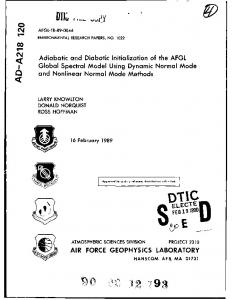
Figure 4. Comparison of TEC measurements from the U.S. Navy Navigation Satellite System (NNSS), TOPEX, and Global Positioning System (GPS) satellite systems at approximately 2320 hours UT on April 3,1994 (left) and on April 5 at approximately 1030 UT (right). very informative, the data gaps near the magnetic equator seriously limit our ability to make precise determinations of the location and shape of the anomaly, particularly in the northern hemisphere. These data gaps are due to the lack of a station near the magnetic equator, together with intermittent power difficulties experienced at the La Paz, Bolivia, station. The dramatic day-to-day variability illustrated in the campaign measurements is consistent with earlier

research. In particular, Wfuden [1993, 1996] reconstructed latitudinal profiles of the maximum F region electron density for 30 consecutive days in September 1958 by combining ionograms from a chain of ionosondes located in the western hemisphere equatorial region. His results illustrate apparent dayto-day differences in the symmetry and magnitude of the equatorial anomaly peaks. He also found asymmetry in the time of the enhancements, where the

as ' I ' ' ' I ' ' ' I ' ' ' I ' ' ' I ' U.T MS

J4.0 _^

[

^^>--_^

-40-2oe>o«i

-40

-«

»

n

*

-M-MOMW

Geomagnetic Latitude Figure 5. Diurnal development of the equatorial anomaly from 1200 to 2400 hours local time for April 4-7,1994.

43

1602

DOHERTY ET AL.: TOTAL ELECTRON CONTENT OVER AMERICAN SECTOR

anomaly peak occurred earlier in the north than in the south for most days in the observation period. The high degree of variation in the development of the equatorial anomaly illustrated in Figure S is primarily due to the large differences in the vertical electrodynamic lift at the equator. Drift variations have been shown to have a large impact on the latitudinal location and amplitude of the equatorial anomaly peaks [Klobuchar et al, 1991]. The symmetry of both the amplitude and position of the equatorial anomaly peaks between the northern and southern hemisphere is largely a neutral wind effect The next section focuses on some of these relationships by comparing campaign data to a theoretical model of the low-latitude ionosphere.

Model Comparisons The data recorded during the campaign provides a unique database for model validation. In this section, a comparison of TEC measurements with calculations from the Phillips Laboratory Global Theoretical Ionospheric Model (GTIM) [Anderson et al, 1996], is presented. The F region portion of this model numerically solves the O^ continuity equation to determine O* densities as a fiinction of altitude, OKf 96 f04/06/»4)

latitude, longitude, and local time. The model requires a variety of geophysical inputs that include a neutral atmosphere, neutral winds, ion and electron temperatures, and E x B drift velocities. The standard model inputs and calculations used in the low-latitude model are described by Preble et al. [1994] and Anderson et al. [1996]. The GTIM model is flexible in that the inputs can be modified to test the sensitivity of the ionosphere to any one or more of these parameters. Figures 6a through 6d illustrate a comparison of the data with a sequence of model calculations. Figure 6a shows the equivalent vertical TEC measurements recorded on April 6. For clarity, the approximate local time is printed near the left y axis and each curve is offset by a factor of 40 TEC units. These data show a well-defined equatorial anomaly at local noon. It peaks near 1900 local time and begins to show signs oi decay at 2300 hours. Figures 6b-6d represent model calculations for comparable geomagnetic, seasonal, and solar conditions. The results shown in Figure 6b are based on a clinutological vertical ExB drift pattern for solar moderate conditions [Fejer, 1981]. Note that the local time development and the dip latitude positions (^ the peaks are realistic, while the magnitudes of the peaks are much smaller than those exhibited in the data measurements. Initial efforts to increase the magnitude MOOa (lEUPERATURE CHANCE)

UOOCL RESULTS I ' I ' I I ' ' I

1

I

I I

I

I

I I

I

I

I

I I

EL (ORin CRAOCNT ADDED) iit| I III ■ I I I I ■ I I 1^ I I

Dip Lotitude Figure 6. (a) Equivalent vertical TEC measurements of April 6, 1994. (b) Model calculations based on climatological ExB drift and original temperature model (see text), (c) Model calculations with a more appropriate low-latitude temperature model, (d) Model calculations with a more appropriate low-latitude temperature model and an £ x fi drift height gradient.

44


1603

of the equatorial anomaly peaks were made by GTIM has shown the capability to reproduce some of increasing the £ x £ drift. The results of those efforts the major features of measured data in the low-latitude (not shown) illustrate larger peaks but with the region, even under geomagnetically disturbed anomaly pushed out to higher latitudes. The base run conditions. of the model shown in Figure 6b used a temperature model that was originally developed for the midlatitude Conclusions region [Strobel and McElroy, 1970]. Figure 6c The first attempt at measuring the day-to-day represents the model calculations that include a more variability of TEC over a large geographic latitude appropriate low-latitude temperature model [Brace and range has been successful. The database collected Theis, 1981]. This modification produces sharper illustrates the large day-to-day variability in the anomaly peaks and more realistic slopes poleward of occurrence, location, and amplitude of the equatorial the anomaly peaks. The dip latitude positions of the anomaly. A surprising feature uncovered by this study anomaly peaks are accurately maintained, but the is that the TEC values are so low in the latitude range magnitude of the peaks are still much smaller than the greater than -t-MO" and that the latitudinal gradients in data calculations. The E x B vertical drift velocities TEC are steeper on the poleward edge of the southern used in the model are based on drift measurements anomaly peak than on the poleward edge of the made at Jicamarca, Peru. In general, they ate applied northern anomaly peak. The multistation data in the GUM model with no altitude dependence. Work measurement technique has been validated by by Pingree and Fejer [1987] and Su et aL [1995] simultaneous measurements of TEC from dualindicate that the altitude variations of the vertical drift frequency GPS and dual-frequency altimeter velocities are important in the development of the measurements from the TOPEX/Poseidon satellite. equatorial anomaly. Figure 6d illustrates model results Model comparisons with observations have when a simple linear height variation in the vertical illustrated, for the first time, the sensitivity of the drift is incorporated into the calculations. This equatorial anomaly to changes in ion and electron modification produces more accurate peak shapes in temperatures and to vertical ExB drift velocities. In both hemispheres and realistic slopes to higher particular, the results show that the altitude variations latitudes within 47-20° dip latitude. The unrealistic of vertical drift velocities have a significant impact on change induced at latitudes greater than ■t-/-20° the development of the equatorial anomaly. Additional indicates that the drift gradient needs to be refined. modeling work is required to fiirther test variations in Although the magnitudes of the anomaly peaks have drift gradients and to investigate neutral wind effects to been increased, they are still lower than the data determine how closely the model can fit the measurements. To provide a more quantitative experimental data over a wide latitude range. measure of the differences shown in Figure 6, plots of One of the prime purposes of the campugn was to data versus model calculations at 1200,1900, and 2300 develop an equatorial database to be used in hours local time are provided in Figure 7. In this ionospheric tomography reconstructions. The study figure, it is evident that the nuxlel calculations that demonstrates that the absence of a station near the include the linear height variation in the drift velocities geomagnetic equator significantly hampers the best replicate the features shown in the data. This is reconstruction of the equatorial ionosphere. Future most apparent at 1900 hours in the northern tomographic campaign organizers, take note! hemisphere and in the shape of anomaly in the modeled results at 1200 and 2300 hours. Appendix: Origin of the Term The comparisons illustrated in Figures 6 and 7 illustrate the sensitivity of the equatorial anomaly to ion 'Êquatorial Fountain** and electron temperatures and E x B drift velocities. Many authors, including Balan and Bailey [1996], Although the data clearly show asymmetries that are have shown that the equatorial fountain greatly likely due to the neutral winds, it is beyond the scope of increases both peak electron density and TEC this paper to replicate this asymmetry with the model. throughout the low-latitude ionosphere; but who Future modeling studies will include efforts to originated this very apt expression for the source of the investigate neutral wind effects and to refme the £ x £ largest ionization in the world? The term "fountain drift gradient applied in the model. In this study. effect" was quoted by Hanson and Moffett [1966,

45


1604

OKt t* 104/M/Ml laia tT

c V

r '• ■—'—r • Campaign Dato .Model Results . Model (Temperature Change) ■ Model (Drift Gradient)

PAY 96 (04/06/94) iJOO IT

DKf 96 (04/06/94) 1900 LT

Compoign Doto > Model Results . _ - Model (Temperoture Change) Model (Drift Gradient)

— Campaign Doto Model Results - . Model (Temperoture Change) Model (Drift Gradient)

E o o UJ

o u

/•/ '^:r.-/-v

r -c-''

«.•«.■ ■■

-M

e

20

DIP LATITUDE

DIP LATITUDE

-4e

' »•

-30

•

■

'

0

20

DIP LATITUDE

Figure 7. Comparison of data versus model calculations at 1200,1900, and 2300 hours local time.

p.5560], as "Martyn (1955) envisages a 'fountain effect' in which the ionization is lifted upward at low latitudes and then deposited at higher latitudes by diffusion along the field lines." Howevra-, the tenn "fountain effecf' is not found in the work by Martyn [1955]. Rush and Richmond [1973, p. 1171] stated "Duncan (1960) has termed this the 'fountain dieory'." HowevCT, the tenn "fountain theoiy" is not found in the woik by Duncan [I960]. After an extensive search, it was discovered that Wright [1962] was the person who coined this term. Wright [1962, p.7], in his discussion of the mechanism producing the equatorial anomaly in F region ionization. stated "We propose the term 'Equatorial Fountain' as a concise term for these processes." Thus the historical record is now set straight

A^nowkdgmcnts. The authors would like to thank the many members of the Ionospheric Effects Division at Phillips Laboratory who participated in the campaign. Air Force Captain William A Pakula deserves particular mention for his outstanding role as Operations Manager for the campaign. Additional appreciation is extended lo Dwight T. Decker of Boston College for many useful discussions on ionospheric nxxicling and to Virginia Ewell and Jane Vladimer of the Electrical, Conoputer, and Systems Engineering Department at Boston University for their assistance in processing the TOPEX measurements used for PANAM data validation. Finally, we would like to thank Jay Spaulding at the U.S. Coast Guard Research and Development Center in Croton, Connecticut, for the loan of the OPS Ashtech tecciva that was used in Merida, Venezuela.

46

References Anderson, D. N., A theoretical study of the ionospheric Fregion equatorial anomaly, I, Theoiy, Planet. Space Sci., 27,409-419,1973. Anderson, D. N., D. T. Decker, and C. E. Valladarcs, Global Theoretical Ionospheric Model (GTIM), in 57£P Hand Book, edited by R. W. Schunk. pp. 133-152, Utah State Univ., Logan, 1996. Balan, N., and G. J. Bailey, Modeling studies of the equatorial plasma fountain and equatorial anomaly. Adv. Space Res., 180). 107-116,1996. Biace, L. H., and R. F. Theis. Global empirical models of ionospheric electron temperatures in the upper F-iegion and plasmasphere based on in situ measurements for the Atmospheric Explorer-C, ISIS-1 and ISIS-2 satellites, J. Atmos. Terr. Phys.. 43,1317-1343.1981. Deshpande, M. R., R. G. Rastogi, H. O. Vats, J. A. Klobuchar, and G. Sethia, Effect of the electrojet on the total electron content over the Indian subcontinent. Nature, 267,599-600,1977. Dimcan, R. A., Hie equatorial F-region of the ionosphere, J. Atmos. Terr. Phys.. 18,89-100, I960. Evans, J. V.. and J. M. Holt, The combined use of satellite differential doppler and groimd-based measurements for ionospheric studies, IEEE Trans. Antennas Propag., AP21,685-692,1973. Fejer, B. G., The equatorial ionospheric electric fields, a review, J. Atmos. Terr. Phys., 43,377-386,1981. Hanson, W. B., and R. J. Moffett, Ionization transport effects in the equatorial F region, J. Geophys. Res., 71 (23), 5559-5572,1966. International Association of Geodesy, International GPS Service for Geodynamics, Cent. Bur., let Propul. Lab., Pasadena, Calif.. 1995.

DOHERTY ET AL.: TOTAL ELECTRON CONTENT OVER AMERICAN SECTOR Imel, D. A., Evaluation of the TOPEX/POSEIDON dual-. frequency ionosphere correction, J. Geophys. Res., 99 (C12). 24.895-24,906,1994. Kersley, L., J. A. T. Heaton, S. E. Pryse, and T. D. Raymond. Experimental ionospheric tomography with ionosonde input and EISCAT verification, Ann. Geophys., 11, 10641074,1993. Klobuchar, J. A.., D. N. Anderson, and P. H. Doherty, Model studies of the latitudinal extent of the equatorial anomaly during equinoctial conditions, Radio Sci., 26 (4), 10251047,1991. Leitinger, R., G. Schmidt, and A. Tauriainen, An evaluation method combining the differential doppler measurements from two stations that enables the calculation of the electron content of the ionosphere, /. Geophys., 41, 201213.1975. Martyn, D. F., Theory of height and ionization density changes at the maximum of a chapman-like region, talcing account of ion production, decay, division, and tidal drift, in Proceedings of Cambridge Conference, pp. 254-259, Phys. Soc., London. 1955. Newton, R. R., The Navy Navigation Satellite System. Space AM.. 7.735-763.1967. Pakula. W. A.. P. F. Fbugere. J. A. Klobuchar. H. J. Kuenzler, M. J. Buonsanto, J. M. Roth, J. C. Foster, and R. E. Sheehan. Tomographic reconstruction of the ionosphere over Nortfi America with comparisons to ground-based radar. Radio Sci., 30 (1), 89-103.1995. Pingree, J. E., and B. G. Fejer, On the height variation of the equatorial F-region vertical plasma drifts. J. Geophys. Res.. 92 (AS), 4763-4766.1987. Preble, A. J., D. N. Anderson. B. G. Fejer. and P. H. Doherty. Comparison between calculated and observed F-region electron density profiles at Jicamarca. Peru, Radio Sci., 29 (4). 857-866.1994. Rastogi. R. G., and J. A. Klobuchar. Ionospheric electron content within the equatorial F> layer anomaly belt, J. Geophys. Res., 95 (All), 19.045-19.052.1990. Rush, C. M.. and A. D. Richmond. The relationship between the structure of the equatorial anomaly and the strength of the equatorial electrojet. /. Atmos. Terr. Phys., 35, 11711180.1973.

47

1605

Sterling, D. L., W. B. Hanson, R. J. Moffett. and R. G. Baxter, Influence of electrodynamic drifts and neutral air winds on some features of the Fi region. Radio Sci., 4, 1005-1023,1969. Strobel, D. F., and M. B. McElroy, The Fj-layer at midlatitudes, Pfcmef. Space Sci., 18,1181-1202,1970. Su, Y. Z., K. I. Oyama, G. J. Bailey, T. Takahashi. and S. Watanabe, Comparison of satellite electron density and temperature measurements at low latitudes with a plasmasphere-ionosphere model, J. Geophys. Res., 100 (A8), 14.591-14,604.1995. Tsedilina, E. E.. O. V. Weitsman, and H. Soicher, Time delay of transionospheric radio signals in a horizontally inhomogeneous ionosphere. Radio Sci., 29 (3), 625-630, 1994. Whalen. J. A., The equatorial F layer: +/- 30° DIPLAT profiles for a continuous 30 day period (abstract). Eos Trans AGU. 74 (43), Fall Meet. Suppl., 457,1993. Whalen, J. A.. Mapping a bubble at dip equator and anomaly with oblique ionospheric soundings of range spread F", J. Geophys. Res.. /0/(A3), 5185-5193.1996. Wright. J. W., Vertical cross sections of the ionosphere across the geomagnetic equator, NBS Tech. Note 138, U.S. Dept. of Commer., Washington, D. C, 1962.

D. N. Anderson, Phillips Laboratory/GPSM. 29 Randolph Road, Hanscom Air Force Base, MA 01731. (e-mail: [email protected]) P. H. Doherty, Institute for Scientific Research, Boston College. St Clement's Hall, Room 402. 140 Commonwealth Avenue, Chestnut Hill, MA 02167. (e-mail: [email protected]) John A. Klobuchar, Total Electronic Concepts, 27 Conant Road. Uncobi, MA 01773. (e-mail:[email protected])

(Received October 10.1996; revised March 3.1997; accepted March 19.1997.)

INTRODUCTION

Description and Assessment of Real-Time Algorithms to Estimate the Ionospheric Error Bounds for WAAS*

The Federal Aviation Administration (FAA) Satellite Program Office is developing a Wide-Area Augmentation System (WAAS) to augment GPS for use during en route through Category I (CAT 1) precision approach flight operations. WAAS has three components: (1) extra ranging sources using geostationary earth orbiting (GEO) communications satellites; (2) a vector of corrections to the GPS signal-in-space, including components for ionospheric delay estimations and clock and ephemeris errors; and (3) an integrity monitoring function to alert users of out-of-toleremce operations. The WAAS will be implemented in three phases. As part of the integrity monitoring function, the WAAS sends to the user a bound on the postcorrection ionospheric vertical error at each of the ionospheric grid points (IGPs) of an ionospheric delay correction grid covering the service area. The ionospheric error bound at each IGP is called the grid ionospheric vertical error (GIVE). The ionospheric delay estimates are used by the user's receiver to correct the pseudorange measurements. Using the appropriate GIVE values, the user also calculates a vertical error bound on ionospheric delay after correction at each of his own ionospheric pierce points (IPPs). This error bound is called the user ionospheric vertical error (UIVE). Any UIVE calculated from the GFVEs must bound the user's postcorrection vertical ionospheric error with a probability of 0.999. Finally, the user calculates a conservative bound of the vertical position error (VPE) using the calculated UIVEs, combined with other error bounds. The requirement for this bound is VPE s 19.2 m. The WAAS Specification [1] was changed in the fall of 1995 to eliminate the initial and end-state GIVE boimds of 2.0 and 1.5 m, respectively. This allowed greater flexibility in meeting the VPE requirement. Nevertheless, some initial analysis has shown that to satisfy the VPE requirement, GIVE values of o.s; 2 O.M VI o.is "" III

0.14

O.tl 0 K 0.11 0.1

■ IIIIIIIIIIIIIIIIIIIIIMHIIIIIIIIIIIIIIMIIIIIIIIIt

ssssssss::s:::ss:: DaU

Fig. 4—Percentage Monitor and User Errors £ UIVE

Figure 5 shows the 95th percentile of GIVEs mapped against the parameter F10.7, which is the solar flux density. The graph indicates the absence of a clear relationship or correlation between solar flux density and ionospheric grid error bounds. The results of [10] also show no correlation between short-term F10.7 and the total electron content (TEC), which is proportional to ionospheric delay. Typical values for F10.7 during solar maximum are between 300 and 350, and about 75 during solar minimum. The reader should be cautioned not to extrapolate the results of Figure 5 to the peak of the solar cycle. Extrapolation is not a substitute for examining data during the peak of the solar cycle.

of the user when the rate is relatively low. For example, on 16 November 1992, the success rate for the user was increased from 97.8 to 98.6 percent, and on 19 November 1992, fit)m 98.97 to 99.46 percent. Table 3 depicts combined results for the several kinds of geomagnetic conditions. During a quiet ionosphere (Ap s 50) and m^jor (not severe) storms (50 < Ap < 100), the 95th and 99th percentiles of GIVE are 1.75 and 2.25 m, respectively. The combined success rate in bounding GIVE for the user is 99.95 percent. During severe geomagnetic storms (Ap > 100), the 95th and 99th percentiles of GIVE are both 5.0 m. The combined success rate for the user is 99.91 percent. Table 4 shows statistical parameters, maximum, and minimum of the distribution of vertical error exceeding UIVE at the monitor (per 5 min update period). The table also shows the same parameters for user error after the maximum monitor error above UIVE for one grid update period has been added to the GIVEs for the next grid update period. It can be seen from this table that when the user error exceeds the UTVEs, the maximum value of the difference between the user error and UIVE is about 0.48 m, and the |mean| + 2 sigma = 0.19 m.

Service Volume Implications

The results in the previous section are conditioned on the existence of at least 1IPP in each of at least 3 grid squares surrounding the IGP in real time. Whenever this condition is not met, the IGP is marked "unavailable." This restriction maintains a high degree of pierce-point density, which favors the calculations in the algorithm. To determine whether this degree of pierce-point density could be maintained in the

Table 3—Combined Resutts Ap Index

GIVE Mean100

1.6

5.0

5.0

99.74

99.91

80.00

Conditions

1.2

Table 4—Error Distribution Above UIVE for Monitor and User Errors at:

Min (m)

Max(m)

Mean (m)

Sigma (m)

Monitor (max) User

0.0011 0.0001

0.4815 0.4815

0.0728 0.0511

0.0964 0.0640

84

Navigation 55

initial WAAS, a map of pierce-point density was constructed using the 24 known sites and the 24 GPS satellites projected to be in operation for the initial WAAS. A modified version of the NAVSTAR program [llj was used to determine how many pierce points would be available every Spring 1997

Si

? 4. > Ô

2.

s ^-

vr ••••'•

80

100

• ■

•« ** •

120

140

%

•

%

160

ISO

F10.7

Fig. 5—Mapping of 95 Percent of GIVE to Solar Flux Density (F10.7)

96 percent of the day. Figure 7 depicts the grid squares (dark) that would be operational based on this condition and the requirement that there be at least 3 surrounding grid nodes with GIVEs in order to calculate UIVEs.

minute in every grid square throughout the day. Next, for each grid node, the percentage of the day was determined for the occurrence of the condition of at least 1IPP in each of at least 3 grid squares surrounding an IGP. For the purposes of this analysis, the following conditional probability relationship was considered:

CONCLUSIONS AND RECOMMENDATIONS

The results of this paper are based on a 52 day set of data. However, the data was from midway through the solar cycle, and includes instances of quiet and disturbed ionospheric conditions. From this, the following conclusions are drawn:

PV[Ionospheric WAAS function available] = Prloverall GIVE s 2.0 m I IPP density requirement satisfied] X Pr[IPP density requirement satisfied]

1) Under nonsevere geomagnetic conditions (Ap s 100), more than 50 percent of CONUS has a pierce-point density that can sustain GIVEs £ 2.0 m 95 percent of the time, and the subsequent UIVEs calculated firom these GFVEs bound the residual user errors an average of 99.95 percent of the time (and never fall below 97.84 percent for any day). This meets the initial WAAS availability requirement of the ionospheric function for precision approach.

= 0.95 Since Prloverall GIVE £ 2.0 m | IPP density requirement satisfied] = 0.988 for nonsevere ionospheric conditions (from Table 3), Pr[IPP density requirement satisfied] must be at least 0.96 for a grid node to be marked as satisfying the density requirement. Figure 6 depicts this condition over the defined service area. Dark circles indicate nodes where the IPP density requirement is satisfied at least 80

-135

-130

-125

-120

-116

Fig. 6—Grid Nodes with Required Surrounding IPP Density

Vol. 44. No. 1

Conker, et al.: Algorithms to Estimate Ionospheric Error Bounds

56

85

•135 -130 -125 -120 -115 -tlO -105 -100

-85

-80

-85

-80

-75

-70

-65

-60

Fig. 7—Grid Squares with at least Three Surrounding Grid Nodes with Required IPP Density

2) For one severe geomagnetic storm (Ap > 100), the 95th percentile of the GIVEs is 5.0 m, and the user's success rate is 99.91 percent. This result means the algorithms were able to detect the change in ionospheric conditions and bound the ionospheric errors with a very high success rate. The impact of such large values of the ionospheric error bounds on the integrity and continuity of WAAS service must be further evaluated. 3) In the few cases where the user errors exceeded the UIVEs, the maximum value of the difference between the user error and UIVE was about 0.48 m, and the |mean| -i2 a was 0.19 m. 4) There is no apparent correlation between solar flux density (F10.7) and ionospheric grid error bounds. Typical values for F10.7 during solar maximum are between 300 and 350, and about 76 during solar minimum. 5) The percentage of the GIVEs below 2.0 m is 98.8 percent for quiet and mtyor (not severe) geomagnetic storm conditions. During the one severe geomagnetic storm for which data was available, this percentage droppped to 80.0 percent. In developing these algorithms, the UIVE bounding requirement was considered to be paramount. The conservative nature of these algorithms, including the density requirement, was considered necessary in order to bound the errors in the test set of data. The density requirement was used to estimate availability in the service volume analysis, and while this meets Phase 1 requirements, availability requirements beyond Phase 1 would not be met without making some 86

Navigation 57

changes. There are several ways this problem could be mitigated: 1) Adding more WRSs to increase the IPP density 2) Reducing the size of the grid (e.g., reducing the spacing between the IGPs) to increase accuracy and reduce errors 3) Allowing more frequent updates to users, especially when the ionosphere is very active Since out-of-tolerance errors tend to persist for longer periods of time than the 10 s measurement update rate, a timely corrective broadcast to users could increase the bounding success rate. This in turn might allow for a slightly less conservative approach in the implementation of the algorithm. ACKNOWLEDGMENTS

The authors would like to acknowledge James K. Reagan and J. P. Femow from The MITRE Corporation, Center for Advanced Aviation S}rstem Development (CAASD), for their review. The authors would also like to acknowledge J. C. Johns and Brian Mahoney of the FAA Satellite Program Office, who were the sponsors of this work. REFERENCES 1. Specification for Wide Area Augmentation System (WAAS), U.S. Department of Transportation, Federal Aviation Administration, FAA-E-2892, May 9, 1994. 2. Wilson, B. D. and Mannucci, A. J., Extracting Ionospheric Measurements from GPS in the Presence of Anti-Spoofing, National Technical Meeting of The Institute of Navigation, September 23, 1994.

. 5

Spring 1997

3. Goad, C. C, Optimal Filtering of Paeudoranges and Phases from Single-Frequency GPS Receivers, NAVIGATION, Journal of The Institute of Navigation, Vol. 37, No. 3, FaU 1990. 4. Eueler, H. and Goad, 0. C, On Optimal Filtering of GPS Dual Frequency Observations Without Using Orbit Information, Bulletin Geodesique, Vol. 65, No. 2, 1991, pp. 130-43. 5. NSTB Software Requirements Specification— Appendix A- Baseline Algorithms, Report No. TR-92072, Stanford Telecommunication Inc., Reston, VA, August 1992. 6. El-Arini, M. B., O'Donnell, P. A., Kellam, P., Klobuchar, J. A., Wisser, T., and Doherty, P. H., The FAA Wide Area Differential GPS (WADGPS) Static Ionospheric Experiment, National Technical Meeting of The Institute of Navigation, January 20-22, 1993, San Francisco, CA. 7. Klobuchar, J. A., Ionospheric Time-Delay Algorithm for Single-Frequency GPS Users, IEEE Transactions on Aerospace and Electronic Systems, Vol. AES-23, No. 3, May 1987, pp. 325-31. 8. Hahn, G. J. and Meeker, W. Q., Statistical Intervals: A Guide for Praetioners, John Wiley & Sons, Inc., New York. 1991. 9. Odeh, R. E. and Owen, D. B., Tables for Normal Tolerance Limit. Sampling Plans, and Screening, Marcel Dekker, Inc., New York, 1980. 10. Klobuchar, J. A. and Doherty, P. H.. The Correlation of Daily Solar Flux Values with Total Electron

Vol. 44, No. 1

Content, Proceedings of the International Beacon Satellite Symposium, MIT, Cambridge, MA, July 6-10, 1992, pp. 192-195. 11. Livingston, R., NAVSTAR program, Stanford Research Institute, February 1977.

ACRONYMS CAT I CONUS DH GEO GIVE GIVE I IGP IPP NSTB PR TEC UDRE UIVE VPE WAAS WMS WRE WRS

Category I Conterminous United States Decision Height Geostationary Earth Orbiting Grid Ionospheric Vertical Error Grid Ionospheric Vertical Error Indicator Ionospheric Grid Point Ionospheric Pierce Point National Satellite Test Bed Pseudorange Total Electron Content User Differential Range Error User Ionospheric Vertical Error Vertical Position Error Wide-Area Augmentation System Wide-Area Master Station Wide-Area Receiver Equipment Wide-Area Reference Station

Conker, et al.: Algorithms to Estimate Ionospheric Error Bounds

58

87

Radio Science, Volume 32, Number 5, Pages 200J-2019, September-October 1997

Improving IRI-90 low-latitude electron density specification Dwight T. Decker Institute for Scientific Research, Boston College, Newton, Massachusetts

David N. Anderson Air Force Research Laboratory, Hanscom Air Force Base, Massachusetts

Amsuida J. Preble Headquarters United States Air Force, Directorate of Weather, Pentagon, Washington, D. C.

Abstract. At low latitudes under moderate to high solar conditions, a number of comparisons between the international reference ionosphere (IRI-90) model of F region electron density profiles and observed profiles measured by tibe Jicamarca incoherent scatter radar indicate that during the daytime the observed profile shape can be much broader in altitude than that specified by IRI-90, while at night, just afber sunset, observed F2 peak altitudes are significantly higher than what is specified by IRI-90. Theoretically derived ionospheric parameters such as F2 peak density (NmP2), -fb peak altitude {hmFz), and profile shape, which are contained in the parameterized ionospheric model (PIM), have been shown in some cases to be in better agreement with Jicamarca observations. This paper describes a new low-latitude option for IRI-90 that uses five ionospheric parameters derived firom PIM: the bottomside profile half thickness, iVm-Fj, KiFi, and two parameters of a topside Chapman profile. The generation of electron density profiles using these five parameters is presented, as well as a description of how these parameters can be implemented into the IRI-90 model. 1. Introduction ™ . , ^, , , . . /ron The international reference ionosphere (IM) w a ôbal empirical model which êcifi,» the monthly average of the electron density, electron temperatiê, ion t^perature, and ion compositaon from 80 to 1000 to. It has been developed as a joint URSI/COSPAR project and first appeared as tables of proffl«presented at the XVH General Assembly of URSI m 1972 However, the general philosophy was to develop a computer model based on critically evaluated obr, . t-^,«Ai»i^1- AmencanGeophysicalUmoii. * • r. I. • ITT • Copyright 1997l»y the " ** Paper number 97RS01029. 0048-6604/97/97RS-01029$11.00

servations, and so IRI quickly evolved from a set of tables to a computer program (IRI-78) ^^ ^^ ^^^ ^^^^ community. Over the ^ ^^ modification of IRI has conJ ^^ ^^^ ^^^.^^ participation by the inter^^ commmiity. The result is that ^^ ^^^^^^ ^^ ^ ^^^^^ ^^^^^^ ,,^,,^ ^^^.^^ ,^_^Q jj^.gg^ 2^.90^ jRj.95) 3^^ has ^^^^^^ ^ ^^^^^ ^^^^ ^î f^,.^.^^^ ,j î ^ ^993. Szuszczemcz et cl., 1996]. ^ ^ data-based model, the IRI is naturally ^^ ^ ^^^ ^ ^^^ available observations. In the case of electron density, . '' the . data . _„^ sources . „„„«. are lonosonde measurements, incoherent scatter measurements, rocket measurements, and a selection of satellite measurements [BiKtza,

2003

59

2004

DECKER ET AL.: IMPROVING IRI-90 LOW LATITUDE IONOSPHERE

1990]. Because the F2 peak parameters (peak density and height) are based on ground-based ionosonde measurements, which are for the most part located in the midlatitudes, there is a lack of observations from the low-latitude regions, the high latitudes/polar cap, and the ocean areas. Likewise, the thickness of the bottomside F region is based on ionosonde measurements and has similar problems in coverage. The topside F region is based on Alouette 1 and 2 topside sounder measurements from 1962 to 1966 [Llewellyn and Bent, 1973]; however, this period included only solar minimum and low solar moderate {FIQ.J < 130) conditions. Given this nonuniform coverage in both location and time of the various databases, it is not surprising that nU does an excellent job of specifying the ionosphere's climatology for some regions and times while having problems with other regions and times. In this paper, we focus on the low-latitude F2 region, a region where IRI has had some success reproducing the general climatology, especizJly for lower levels of solar flux, but where there are some persistent disagreements between model and observations [Ahdu et a/., 1996]. Early work based on total electron content (TEC) measurements found examples at low latitudes where IRI "severely underestimated" the observed TEC "during both day and night" [Bilitza, 1985, p. 15]. Analysis of these cases suggested that the problem was in the relative shape of IRI's F2 region at low latitudes. The topside of this layer comes from the Bent model [Llewellyn and, Bent, 1973], and a correction to IRI's implementation of that model appeared in IRI-86. While this produced better agreement with satellite and incoherent scatter data, it was noted at the time that the new topside formula "only removed half of the difference between measiu-ed and predicted" TEC at the magnetic equator [Bilitza, 1985, p. 18]. Further, while IRI-86 appeared to do a reasonable job at low solar activity, comparisons with in situ satellite measurements during high solar activity indicated that ERI's topside profile still significantly underestimated the observations [Bilitza et al, 1987]. The other half

60

of the "shape of the F2 region" is the bottomside of the F2 layer, which is described by an analytic function parameterized in terms of a tluckness parameter for which IRI offers two options. The reconmiended option in most cases comes from the Gulyaeva et al. [1987] model for the half-density height. However, this bottomside thickness has also had some problems at low latitudes. Mahajan et al. [1995] showed, using Arecibo incoherent scatter radar data, that IRI produced a bottomside that was too thick by differing amounts depending on season, and improvements to IRI have been suggested based on this work [Gulyaeva et al, 1996]. Comparisons to dlgisonde data from Jicamarca [Reinisch and Huang, 1996] have likewise shown some differences between data and IRI, with the most dramatic differences occurring in August 1993 when ERI's bottomside F2 layer was seen to be tens of kilometers thinner than observed. Finally, we turn to the F2 peak density (NmFi) and height {hmF2), which are used in IRI to complete the definition of the F2 region. For these two paranieters, the most persistent problem at low latitudes has been with hmF2 and in particular the inability of IRI in certain periods to reproduce the observed rising in altitude of the F2 layer just after sunset [Bilitza et al, 1993; Abdu et al, 1996]. As mentioned, the soturce of these problems is the nonuniform coverage of the available data. This is a particular problem at low latitudes because vertical E x B drift leads to the formation of the equatorial anomaly and the development of a complex morphology quite different from that of the midlatitudes. However, the problems at low latitudes are also exacerbated by the large day-to-day variability of this region. In particular, it is problematic at best to attempt to model a feature such as the equatorial anomaly in terms of monthly medians when all the characteristics of the anomaly (intensity, location, extent, latitudinal shape) are known to VEiry greatly day to day. For example, owing to the changing position and extent of the anomaly, a single low-latitude groimd station can day to day effectively be sampling different geophysi-

DECKER ET AL.: IMPROVING IRI-90 LOW LATITUDE IONOSPHERE czJ regions. Assembling data averages from several such stations can result in a smeared out anomedy that is not representative of an actual anomaly [Rawer, 1995]. While for some purposes such an average ionosphere is all that is needed, for other uses it is critical to have a representative, or "typical," ionosphere. One effect of the issues described above is that theoretical modeling has begun to appear as a complementary approach to strict empirical modeling. Rush et al. (1983, 1984] used theoretical modeling to fill in the data gaps over the midlatitude oceans and, along with groundbased ionosonde observations, produced an improved set of maps of the F2 peak critical frequency {foF2)- Such maps are the sources used by nil for foF2 and hence NmF2- Further improvements to the f„F2 maps were made using theory over the oceans, a larger database of ionosondes, and a harmonic analysis that was latitude dependent [Fox and McNamam, 1988]. At about the same time, efforts appeared that used first-principle theoretical models to produce parameterized models that would describe low-latitude theoretical morphology [Anderson et al, 1987, 1989]. The purpose was to produce

2005

a representative equatorial anomaly rather theui a smeared out average anomaly [Daniell et al, 1995]. In this paper, we propose a new option for IRI which would allow the results of loiw-latitude theoretical modeling of electron density to be incorporated directly into IRI. The purpose is to provide an improvement to IRI as well as to illustrate one way in which our theoretical imderstanding can be used to fill in the gaps of the observational databases used by IRI. In the next section, we present some observations compared with IRI-90 in order to quantitatively illustrate some of problems outlined above. This is followed by a description of the theoretical modeling of the low-latitude ionosphere, an example of a parameterized ionospheric model (PIM) option to nU, and finally, a discussion and conclusion section.

2. Observations Having qualitatively described some of the disagreements between IRI and observations at low latitudes, in this section we use comparisons between the Jicamarca incoherent scatter radar observations and IRI-90 to give quantitative examples of these disagreements. In Figure 1, we

b)1900LT

a)1200LT

I 10^ 10^ density (cm"^)

-3> density (cm"^)

Figure 1. Comparison of Jicamarca observed profiles and IRI-90 (international reference ionosphere) profiles for October 1 and 2, 1970, at (a) 1200 LT and (b) 1900 LT. The solid curves are the observations, and the dashed curves are IRI-90.

61

10"^

2006


(a) Dec. solstice

density (cm'^)

(b) Equinox

(c) June solstice

density (cm'-')

10^ 10^ density (cm"^)

10'^

Figure 2. Seasonal comparison of IRI and parameterized ionospheric model (PIM) with Jicamarca average profile for 1200 LT, solar moderate conditions for (a) December solstice, (b) equinox, and (c) June solstice. The solid curves axe observed average profiles (100 < Fio T < 150), the long dashed curves are IRI (sunspot = 80), and the dotted curves are PIM (Fxo.7 = 128). present an example of an electron density profile observed on October 1 and 2, 1970, during moderate solar conditions by the Jicamarca radar, which is located near the magnetic equator in Peru. Also included in the plot are IRI-90 profiles that were produced assuming a sunspot number of 80 (F10.7 = 130). At 1200 LT the observed profile has a broad shape that is fairly tjrpical of the dajrtime profile shape seen at Ji-

(c) June solstice

(b) Equinox

(a) Dec. solstice


camarca during solar moderate and maximimi conditions. On the other hand, IRI-90 has the thinner shape more characteristic of solar minimum, as well as an increased scale height above 700 km that suggests a transition from an O"*" dominated F region to a H"*" dominated topside. Later in the day, at 1900 LT the observed layer has been lifted to much higher altitudes due in most part to an observed enhanced postsimset E

10*^

10^ 10^ density (cm"-')

16^

Figure 3. Same as Figure 2 but for 1800 LT.

62

10^ 10^ density (cm'^)

10'^


(a) Dec. solstice

10^ 10^ density (cm'-')

(b) Equinox

10^


2007

(c) June solstice

10'^


10^

Figure 4. Same as Figure 2 but for 2000 LT. X B upward drift. This again is a characteristic feature of the Jicamarca reôn, especially during solar moderate and maximum periods, and again is a feature not reproduced by IRI-90. The point of the above comparison is to simply illustrate the type of problem that can be encountered at low latitudes when comparing IRI and actual observations. However, given that nU is a model of monthly profiles, it should not be expected to necessarily reproduce the profiles on a given day. While the broad shape of the afternoon profiles and the postsunset lifting of the layer are not rare events and occur regularly, in order to validate that IRI has in fact a low-latitude problem, comparisons need to be made between some sort of averaged data and IRI. In Figtures 2-4, which are adapted &om Cnamer [1992], we show the hourly averaged data from several years of Jicamarca observations for moderate solar flux conditions. December solstice refers to data taken during November through February, and June solstice refers to data from May to August. The equinox period was taken to be March and April along with September and October. These plots also include results from IRI-90 and the parameterized ionospheric model (PIM). In this section, we will focus on the data (solid curves) and IRI90 (dashed curves) results. PIM results (dotted

63

curves) will be discussed in the following section. The IRI runs were made using a sunspot number of 80 and for days of the year 1, 100, and 182. The data are from days where the F10.7 ranged from 100 to 150. We begin by noting that the observed profiles (solid curves) are generally broader than IRI-90 (dashed curves), though in several cases IRI-90 does a reasonable job. In Figure 2 (1200 LT) we see that for December solstice, the shape of nU's profile compares quite well with the averaged data. At equinox, we begin to see some differences in both the topside and bottomside shapes between IRI and data. For June solstice, the differences in the bottomside shape are most apparent. In Figture 3 (1800 LT) we see similar trends, with clear differences between IRI90 and data in topside shapes during December solstice and equinox and bottomside differences during June solstice and equinox. Finally, in Figure 4 (2000 LT), the postsunset lifting of the layer is evident (soUd curves) during December solstice and equinox and is seen to be missed by IRI-90 (dashed curves). There is a smaller amount of lifting of the layer for June solstice, but it is difficult to see given that the data were placed into 40-km bins when producing these average profiles. If hjnFz is taken from the unbinned data and then averaged, the Jtme solstice


2008

results then show a peak rise of just 16 km between 1700 and 2000 LT. In contrast, equinox shows a 55-km increase. Similar features are seen for maximum solar flux conditions but not for solar minimum conditions. IRI-90 also consistently shows an increased scale height above 700 km. While the data show some evidence that this is not the case (see equinox at 1200 and 1800 LT), in general, these observations are too low in altitude to clearly determine whether this increased scale height is appropriate. While the observations shown thus far come from one location, similar features are also evident in other longitude sectors. Many of the works referenced in the introduction describe studies that included data from other longitude sectors. In Figure 5, we present profiles (R. Tsunoda, personal communication, 1995) observed by the Kwajalein incoherent scatter radar located near the equator in the Pacific sector. On the left is a profile from the early morning before upward drift E x B drift has acted to broaden the peak, while on the right we see later in the day the characteristic broad layer of the low-latitude daytime that results from the upward E X B drift. Further, it has been clearly established that the equatorial anomaly is global in nature [Wôflber, 1981; Su et ai, 1996] and that the E x B drift, though different in detail,

is similar at all longitudes [Fejer et al, 1995]. Given that the discrepancies described above are related to the effects of vertical E x B drift and the equatorial anomaly, it is then consistent that nU would have these low-latitude problems at other longitudes. 3. Theoretical Modeling Over the last three decades, there have been many theoretical studies of the equatorial F2 region, and a number of computer models have been developed that reproduce the basic features of this region. Most recently, these models have evolved to the point that given realistic inputs for a particular day, they are capable of reproducing the ionosphere of that day [Pre6/e et ai, 1994]. One such model is the global theoretical ionospheric model (GTIM), which calculates electron density profiles as a function of location and time by solving ion continuity and momentum equations. For the F region, the O"*" ion density is determined by ntunerically solving the time dependent ion (O"*") continuity equation. The needed velocity parallel to the magnetic field comes from combining the electron and ion momentum equations. The perpendicular velocity is taken as the E x B drift where the electric field has to be provided as an input

1000

1000

I 10^ 10^ density (cm'^) Figure 5.

density (cm"^)

Electron density profiles observed by Kwajalein incoherent scatter radar.

64


to the model. A variety of other geophysical inputs are also required, including the neutral constituents, temperature, and winds; the electron and ion temperatures; the solar extreme ultraviolet (EUV) fluxes; and the geomagnetic field. For the lower altitudes, the molecular ions are determined by nimierically solving the steady state local approximation of four coupled ion continuity equations [Anderson et a/., 1996]. In Figure 6, we present vertical profiles for 1200 and 1900 LT from GTIM simulations (dotted curves) that used the Jicamarca observed upward E X B drift of October 1 and 2, 1970. We also include in the plot the electron density profiles (solid curves) observed by the Jicamarca radar at thdse times. We see that when the observed drift is used as an input to the model, the agreement between model and observation is excellent. Further, we see that the model reproduces both the broad profile shape of the daytime and the lifting of the F2 layer during the poststmset period. The additional ciirves (dashed curves) are GTIM results when zero vertical E x B drift was used as input. These simulations Illustrate the critical role that

1000

2009

the magnitude of the E x B vertical drift has in determining both the shape of the daytime profile and the postsunset rising of the F2 layer. Recently, a computationally fast parameterized ionospheric model (PIM) was developed at the Phillips Laboratory Geophysics Directorate as part of a global, real-time ionospheric specification model called PRISM (parameterized real-time ionospheric specification model) which is presently operational at the Air Force 55th Space Weather Squadron (55SWX) in Colorado Springs [Daniell et o/., 1995]. PIM is based on many runs of several theoretical ionospheric models and as such is a global ionospheric model based on theoretical climatology rather than empirical climatology. For the low latitudes, the theoretical model used was an early version of GTIM. It was run under three solar cycle conditions (low, middle, and high Jîo.7 cm flux values) and three seasons (fall-spring equinox, summer, and winter solstice periods) for foUr longitude sectors (American, Brazilian, European-Indian, and Pacific). Electron density profiles every 2° latitude and every hour local time were parameterized by nine empirical orthonormal func-

b)1900LT

a)1200LT


10'^


Figure 6. Comparisons of measured and calculated profiles on October 1 and 2, 1970, for (a) 1200 LT and (b) 1900 LT. The solid curves are the Jicamarca observations, the dots are calculations that used observed drifts, and the long dashes are the calculations using zero drifts.

65

10'^

2010


tions (EOFs). At low and middle latitudes these EOFs were analytically fit in latitude and kept in tabular form over the 24-hour period. These tables and functions comprise the low-latitude portion of PIM and reproduce very accurately the electron density profiles generated by GTIM. Given the success of theoretical models in reproducing the basic features of the low latitudes, we would expect that PIM should likewise reproduce those features. In Figures 2-4, we have included PIM results (dotted curves) along with the averaged Jicamarca data (solid curves) and the IRI-90 (dashed curves) results. In Figure 2 for December solstice, we see that PIM produces a profile that is broader than the data. Both PIM and IRI-90 underestimate TV^-Fb, and to some extent the topside and bottomside data seem to split the difference between PIM and IRI-90. At equinox, PIM's (dotted curve) topside shape gives good agreement with data (solid curve) up to around 600 km. Above that height, both PIM and IRI miss the sharp faUoff in the data. Again in the bottomside, the data split the difference between the models, though if we normalize IRI to the F2 peak of the observations, IRI (dashed curve) has the better bottomside shape. Finally, for June solstice, PIM produces a broader layer than IRI-90, with the data falling between the two models. However, this time it is PIM that has the better bottomside shape, with IRI-90 showing a much thinner bottomside than seen in the data. T\iming to Figure 3 and 1800 LT, we again see a broader FW[ (dotted curves) as compared with IRI-90 (dashed curves). For December, PIM's topside agrees quite nicely with the data, while IRI-90 shows a significantly different shape. Moving to equinox, up to around 600 km, PIM gives reasonable agreement with the observed topside, but as was the case at 1200 LT, both PIM and IRI-90 miss the sharp falloff seen in the data at higher altitudes. In the bottomside the observed layer appears to be a bit thicker than either model. June solstice again shows an observed topside shape that falls between the two models and an observed bottomside shape that

66

is thicker than either model. At 2000 LT (Figure 4), similar trends continue. PIM gives good agreement with observations over much of the F region. In particular, PIM captures the lifting of the layer that was missed by IRI-90. For equinox, PIM captures the topside shape and the lifting of the layer. However, both IRI90 and PIM produce much thinner bottomsides than seen in the averaged data. Finally for June solstice, PIM shows a layer that has risen to a higher altitude (/im-^2 « 440 km) than that seen in the observations (/im^2 « 410 km), while IRI90 is down at a lower altitude (/im-Fa w 355 km). Having seen how both IRI and PIM compare with data from Jicamarca for solar moderate conditions, let us now compare the two models over a larger region and for solar maximum conditions (fio.7 = 200), In Figure 7, we directly compare PIM and IRI-90 profiles at 1700 UT in Jicamarca longitude meridian. The local time is 2u:oimd 1200, and we see that PIM produces a much broader F layer around the magnetic equator than does IRI-90. However, the PIM anomaly falls off much faster with latitude than does IRI-90 so that 20° north of the magnetic equator (aroimd 10° north geographic) IRI-90 is producing a thicker layer. This illustrates how in regions of great variability, theoretical models can produce sharper features (in this case an anomaly that is narrower in latitude) than may be seen in models based on averaged data. In Figure 8, it is /im-^b that is compared over the entire globe at 0000 UT, and we see that the largest differences between PIM and IRI-90 are confined to the postsunset period near the equator. The topside half thicknesses are compared in Figure 9, and here a sizable difference is seen near the magnetic equator but extended over 180° in longitude. This also points out how the differences in thickness between models are not confined to just one longitude sector. In Figure 7, a clear difference in layer thickness was seen in the American sector at 1700 UT. At 1200 UT, this difference is seen in the European-Indian sector.

DECKER ET AL.: IMPROVING mi-90 LOW LATITUDE IONOSPHERE

2011

PMEDP

I^ 500 s

LogNe 6.375 6.35 ■10

6.325

0 10 Geographic Latitude

6.3 6.275

IRIEDP

6.25 J 6.225 -^6.2

-10 0 10 Geographic Latitude

20

30

Figure 7. Electron density in the Jicamaxca longitude meridian from PIM and niI-90 for 1700 UT (1200 LT) under solar maximum conditions (iîo.T = 200) on day 100.

67


2012

PIMhniF2

hinF2 (km) 700 650 0

50

100

150 200 250 Geographic Longitude

300

350

600 550

IRIhmFz

i-500 450

100

150 200 250 Geographic Longitude

300

350

Figure 8. Values of ftmFj from PIM and IRI-90 for 0000 UT under solar maximum conditions (F10.7 = 200) on day 100.

68

2013


PM Topside Half Thickness I

I

I

I

^ I

I

11 I

I

j

I

Y

I

I

zhft(km) 300

100

150

200

250

300

350

Geographic Longitude Figure 9. Topside half thickness from PIM and IRI-90 for 1200 UT under solar maximum conditions (FIO.T = 200) on day 100.

69

2014


4. Proposed Improvement to IRI-90: PIM Option

three are given as functions of geomagnetic latitude, solar flux, and foF2. (This profile can be described in terms of a linear combination of In describing the electron density profile from LAY-functions [Bilitza and Rawer, 1990].) The 80 to 1000 km, IRI-90 uses six subregions: the bottomside is given by a fairly simple ftmction topside, the F2 bottomside, the Fi layer, the which, as mentioned, uses a thickness parameintermediate regions, the E valley, the E botter. The present IRI-90 either looks up this patomside, and the D region. The upper parts rameter or calculates from a half thickness from of this profile are in turn normaUzed to the F2 Gulyaeva et al [1987]. The PIM option would peak density (NmFz) and altitude {hmF2). The involve using PIM values for NmF2, /im-p2» and difficulties described in this paper have involved bottomside half thickness directly in IRI. The the topside and F2 bottomside regions as well a^ hmF2, and it is these quantities for which we difficulties discussed have not focused on NmFi, propose an alternative source that we call a PIM but we have included it as part of the PIM opoption to mi. In IRI, NmF2 comes from either tion so that it would include a complete indethe CCIR or URSI coefficient sets that derive pendent F region. To use the topside from PIM from Fourier and spherical harmonic expansions in IRI will require either fitting Booker functions of ionosonde data. Likewise, there are CCIR to PIM profiles or fitting with some other funccoefficients of M(3000) which are used to infer tion that would then have to be incorporated hmF2' The topside profile shape comes from into mi. Presently, IRI-90 allows inputting of a NmFz analytic fits of Bent's compilation of Alouette and kmF2 chosen by the user. To input a botsounder data [Llewellyn and Bent, 1973]. The tomside half thickness chosen by the user refits are done using Epstein functions which can quires modifications of the mi driver routine be used to define a Booker function. The Booker such that a user-specified thickness can be acftmction used in IRI-90 consists of three layers, and it uses eight parameters to define the profile. cepted and substituted for the Gulyaeva et al. Five of the parameters are fixed, and the other [1987] thickness. For the topside, we have ex-

b) IRICFEVIFJ + PIM

a) IRI + PIM

3 •a



Figure 10. Comparisons under solar maximum conditions (FIO.T = 200) at 2000 LT of IRI-90 and PIM profiles for (a) standard IRI and (b) IRI using PIM F2 peak parameters. Solid curves are IRI-90, and dashed curves are PIM.

70

2015


plored one possibility by fitting topside PIM profiles with two-parameter Chapman profiles. The IRI driver was modified to accept these two parameters, and a routine was added to IRI to caictdate the topside profile using a Chapman profile rather than a Booker function. Overall, the examples in this paper required only 20 lines of new code to IRI-90. An example of how this approach can allow IRI to reproduce PIM profiles using the five PIM parameters is given in Figures 10 and 11. In Figure 10a, we present the standard IRI-90 (solid curve) and PIM (dotted curve) profiles for 2000 LT at the magnetic equator for solar maximum conditions (F10.7 = 200). We see a dramatic difference in both shape and hmF2- Figure 10b shows PIM compared with IRI-90 using NmFi and htnF2 supplied by PIM. When the PIM bottomside half thickness is used by IRI-90, we see in Figure 11a that IRI-90 now reproduces well the lower F region of PIM. Finally, in Figure lib, the PIM topside profile is also used by IRI-90, and we see that IRI using the full PIM option can do a reasonable job at reproducing the original PIM F region. The next step in developing a global PIM option will be to determine the five PIM param-

a) IRI(PIMF2+Zb) + PIM

eters over the globe under various geophysical conditions. It is expected that the resultant database of parameters will then have to be condensed to a convenient size. One possibility would be to fit the five PIM parameters to analytic functions in the same way as was done with the F2 peak parameters derived from ionosonde data (CCIR or URSI coefficients). Whether this is a feasible approach wiU require further work. Finally, while the focus in this paper is on low latitudes, we should note that at the 1994 COSPAR meeting in Hamburg, Germany, the IRI community endorsed developing a highlatitude PIM option to the IRI model. Given this fact, it would seem best to develop a global PIM option for IRI. This would avoid the problem of attempting to merge a PIM option in one region with standard IRI in other regions. 5. Discussion and Summary At present, there are some clear shortcomings in IRI's description of the low-latitude ionosphere. On the other hand, theoretical models have been shown capable of reproducing some of the low-latitude features that are not repro-

b)IRI(PIMpar) + PIM 1000

I 13

10^

10^

density (cm'^)

density (cm*^)

Figure 11. Comparisons at 2000 LT of IRI-90 and PIM profiles for (a) IRI using PIM Fj peak parameters and bottomside half thickness and (b) IRI using all five PIM parameters. Solid curves are IRI-90, and dashed curves are PIM.

71

2016


duced by IRI-90. In particular, for periods of ter radar. Further validation for the PIM option moderate to high solar activity, PIM has been awaits other data sources. One near-term possishown to produce a broader F region than IRI bility is the TEC observations that are available and to capture the observed postsunset rising from the dual-frequency, dispersive radar on the of the F2 layer. Given these facts, it has been TOPEX/Poseidon satellite [Bilitza et a/., 1996]. suggested that it would be useful to develop a These observations, which began around the below-latitude PIM option to the IRI model. This ginning of 1993, would appear to offer an excitsuggestion was considered and endorsed by the ing opportunity for low-latitude testing of IRI, mi community at the 1995 IRI meeting in New PIM and GTIM. Delhi, India. This low-latitude option will be A key issue when considering the validation part of a global PIM option being developed by of models such as IRI or PIM is that of dayPhillips Laboratory, and the global option will to-day variability. This is especially critical in be delivered to the IRI community when com- a region, such as the low latitudes, where that variability can be quite large. This issue manpleted. The present version of IRI-90 is designed to ifests itself in several ways. For example, the accept NmF2 and hmFz from outside sources. process by which one constructs an average from Thus it is straightforward to develop a PIM op- data becomes critical, especially if dealing with tion for these parameters in IRI-90. Similarly, any type of variable structure. As mentioned an external bottomside half thickness can easily in the introduction, the latitude extent of the be incorporated into IRI-90, given the manner anomaly can easily be smeared out if one takes in which IRI-90 presently defines its bottomside routine averages of ground-based meastu-ements. F region. Unfortunately, the parameter which Another example is that of the shape of the altiis most in need of modification is the topside tude profile changing markedly from day to day half thickness. Presently, there is no trivial way even when the solar and magnetic conditions are of incorporating such a thickness from another not markedly different. In that case an "aversource such as PIM into the IRI. However, a age profile" may represent only one of the posfairly minor modification is possible that uses a sible profile shapes. In Figure 2 for December two-parameter Chapman profile rather than the solstice, we see an average profile with a topBooker functions. If use of the Booker functions side shape falling between niI-90 and PIM. If is desired, then such functions would have to one examines the scatterplots of the 18 profiles be fit to PIM profiles. Presently, we are most that went into making up this average [Creamer, interested in pursuing the option that uses the 1992], one sees a range of profiles that go from Chapman profile and in developing representa- very broad shapes, low peak densities (7.0 x 10^), tions of the five PIM parameters as functions of and high hmF2 (>400 km) to thin topsides (thinlatitude, longitude, local time, solar cycle, sea- ner than IRI), high peak densities (2.5 x 10^), and lower Am-Fb (~325 km). In this case, both son, and geomagnetic activity. While we have demonstrated the possibility IRI and PIM fall within this range of profile and potential of the PIM option, the same type shapes. We can speculate that the PIM proof validation is needed for PIM as is necessary for file's shape is representative of those days when any version of IRI. However, validating the PIM the electric field was of a certain strength, while option faces the same problems that have ham- IRI being based on solar minimum data possibly pered IRI validations, that is, the availability of represents those profiles from days with weaker suitable observations. To date, validation of the electric fields. However, all the cases fall into low-latitude portion of PIM has been confined to the same category of magnetically quiet, modthe American sector, primarily to comparisons erate solar conditions. Of course, with such a with data from the Jicamarca incoherent scat- range of shapes, it is difficult to determine what

72

DECKER ET AL.: IMPROVING IRI-90 LOW LATITUDE IONOSPHERE is "typical," and there is little reason to expect that a theoretical model driven by an average E X B drift based on one limited set of drift data will necessarily produce the "average" seen in a limited set of electron density profile data from a different period. In such regions with large variability, what is needed for IRI is an expanded capability that quantifies the variations about the "average profile." As for PIM, it is planned that the next version will be parameterized by an electric field strength parameter. In order to validate such a version of PIM and the above speculation, it would be useful to perform a GTIM model study where a database of simultaneous vertical drift and electron density profile measurements is available. In that case, one could verify whether the observed day-today variations in profile shape can be modeled as directly coming from the observed day-to-day variations in vertical drift. The scale height differences above 700 km between the IRI-90 and PIM profiles are an obvious issue that needs to be addressed as we consider the issue of model validation. As mentioned in section 2, the increased scale height shown in IRI-90 suggests a transition from an 0+ dominated F region to a H+ dominated topside. This suggestion comes from both theory and observations that have shown that this type of scale height change occurs when this transition of species occurs [Bilitza, 1990]. Further, the transition heights observed at solar minimum are generally consistent with the transition heights evident in the IRI-90 profiles. That this is so is, of course, reasonable, given that IRI's topside is based on solar minimmn topside sounder data. However, observations have shown that the transition height moves up in altitude at higher levels of solar activity. This has been verified recently in a study of DMSP satellite data [West et of., 1997] that showed during low solar activity the transition height is well below 800 km and is well above 800 km during higher solar activity. Further, for the times of the DMSP data, it was seen that the H+ density at 800 km never gets much above 1 or 2 x 10* .

73

2017

In disagreement with this are the IRI-90 results which show for solar moderate conditions at 2148 LT (the time of DMSP data) a scale height change at aroimd 700 km and H+ densities at 800 km of around 9 x 10*. An observational solution to this problem should come from topside sounder data. However, only a small part of the Alouette-iSIS topside sounder database has been available for use [Bilitza, 1994]. It is expected that if and when more of this database becomes available, significant improvements can be made in IRI's topside morphology. On the theoretical side, we find that PIM does not include H"^ and so obviously cannot describe the transition between species. Fortimately, the new version of GTIM under development includes H"*" at low and middle latitudes. It is anticipated that the next version of PIM will be produced using this improved GTIM and thus should include the transition from 0+ to H+ that occurs in the topside. The two issues discussed above (daily profile shape changes and 0'*'/H"'' transitions) are examples of the problems that arise in part from the lack of suitable databases. They are also examples of where theoretical models could be used to complement pure empirical modeling. That is, validated theory can serve to fill m the data gaps and provide a spatial and temporal framework when the databases are too sparse to do so. We expect that a next generation PIM that includes both H"*" and an electric field parameterization can play such a role and serve to complement strict empirical modeUng. Finally, this work was done using IRI-90; however, during the writing of this paper, IRI-95 became available and could be nm interactively via a World Wide Web site. We have rerun the cases shown in Figures 2-4 using IRI-95 and find essentially no differences in the topside and F2 peak parameters. However, for days 1 and 100, the bottomsides at 1200 LT commg from IRI-95 are somewhat thinner than the IRI-90 results. Given these results, it is evident that essentially all our conclusions based on IRI-90 remain true for IRI-95.

2018


Acknowledgments. The work at Boston College waa supported by Phillips Laboratory contracts F19628-93-K0001 and F19628-96-C0039.

References Abdu, M. A., I. S. Batista, and J. R. de Souza, An overview of IBI-observational data comparison in American (Brazilian) sector low latitude ionosphere, Adv. Space Ret., 18{6), 13-22, 1996. Anderson, D. N., M. MendiUo, and B. Hemiter, A semi-empirical low-latitude ionospheric model. Radio Sci., 22, 292-306, 1987. Anderson, D. N., J. M. Forbes, and M. Codrescu, A fully analytical, low- and middle- latitude ionospheric model, J. Geophya. Res., 94, 1520-1524, 1989. Anderson, D, N., D. T. Decker, and C. E. Valladares, Global theoretical ionospheric model (GTIM), in Solar-Terrestrial Energy Program: Handbook of Ionospheric Models, edited by R. W. Schunk, pp. 133-152, Natl. Oceanic and Atmos. Admin., Boulder, Colo., August 1996. Billtza, D., Electron density in the equatorial topside. Adv. Space Res., 5(10), 15-19, 1985. Bilitza, D., International reference ionosphere 1990, NSSDC/WDC'A-R&S Rep. 90-22, Goddard Space Flight Cent., Greenbelt, Md., 1990. Bilitza, D., Topside models: Status and future improvements, Adv. Space Res., i^(12), 17-26,1994. BiUtza, D., and K. Rawer, New options for IRI electron density in the middle ionosphere, Adv. Space Res., 10{n), 7-16,1990. Bilitza, D., K. Rawer, S. Pallaschke, C. M. Rush, N. Matuura, and W. R. Hoegy, Progress in modeling the ionospheric peak and topside electron density. Adv. Space Res., 7(6), 5-12,1987. Bilitza, D., K. Rawer, L. Bossy, and T. Gulyaeva, International reference ionosphere - Past, present, and future, I, Electron density, Adv. Space Res., 1S{3), 3-13, 1993. Bilitza, D., C. Kobllnsky, S. Kia, R. Williamson, and B. Beckley, The equatorial anomaly region as seen by the TOPEX/POSEIDON satellite, Adv. Space Res., 18{6), 23-32, 1996. Creamer, A. P., Equatorial f-region electron densities over a solar cycle: Comparisons between observations and numerical models, M.S. thesis, 201 pp., Utah State Univ., Logan, 1992. Daniell, R. E., Jr., L. D. Brown, D. N. Anderson, M. W. Fox, P. H. Doherty, D. T. Decker, J. J.

74

Sojka, and R. W. Schunk, Parameterized ionospheric model: A global ionospheric parameterizar tion based on first principles models, Radio Set., SO, 1499- 1510, 1995. Fejer, B. G., E. R. de Paula, R. A. Heelis, and W. B. Hanson, Global equatorial ionospheric vertical plasma drifts measured by the AE-E satellite, /. Geophys. Res., 100, 5769-5776,1995. Fox, M. W., and L. F. McNamara, Improved worldwide maps of monthly median foF2, J. Atmos. Terr. Phys., 50, 1077-1086,1988. Gulyaeva, T. L., Progress in ionospheric informatics based on electron-density profile analysis of ionograms. Adv. Space Res., 7(6), 39-48, 1987. Gulyaeva, T. L., K. K. Mahajan, and N. K. Sethi, Modification of IRI half-density height option for low latitudes. Adv. Space Res., 18(6), 149-152, 1996. Llewellyn, S. K., and R. B. Bent, Documentation and description of the Bent ionospheric model. Rep. AFCRL-TR-7S-0657, Air Force Geophys. Lab., Hanscom AFB, Mass., 1973. Mahajan, K. K., R. KohU, N. K. Sethi, and V. K. Pandey, Variability of the F-repon parameter hO.5, Adv. Space Res., 1S{2), 51-60, 1995. Preble, A. J., D. N. Anderson, B. G. Fejer, and P. H. Doherty, Comparison between calculated and observed F region electron density profiles at Jicamarca, Peru, Radio Sci., 29, 857-866,1994. Rawer, K., Ionospheric mapping in the polar and equatorial zones. Adv. Space Res., 16 (1), 9-12, 1995. Reinisch, B. W., and X. Huang, Low latitude digisonde measurements and comparison with IRI, Adv. Space Res., 18(6), 5-12, 1996. Rush, C. M., M. PoKempner, D. Anderson, F. G. Stewart, and J. Perry, Improving ionospheric maps using theoretically derived values of foFj, Radio Sci., 18, 95-107, 1983. Rush, C. M., M. PoKempner, D. Anderson, J. Perry, F. G. Stewart, and R. Reasoner, Maps of f^Fi derived from observations and theoretical data. Radio Sci., 19, 1083-1097, 1984. Su, Y. Z., K.-L Oyama, G. J. BaUey, S. Pukao, T. T^kahashi, and H. Oya, Longitudinal variations of the topside ionosphere at low latitudes: Satellite measurements and mathematical modelings, J. Geophys. Res., 101, 17,191-17,205,1996. Szuszczewicz, E. P., et al., F region climatology during the SUNDIAL/ATLAS 1 campaign of March

DECKER ET AL.: IMPROVING mi-90 LOW LATITUDE IONOSPHERE

2019

1992: Model-measurement comparisons and causeeffect relationships, /. Geophya. Res., 101, 26,74126,758,1996. Walker, G. O., Longitudinal structure of the Fregion equatorial anomaly - A review, J. Atmos. Terr. Phya., 43, 763-774,1981. West, K. H., R. A. Heclis, and F. J. Rich, Solar activity variations in the composition of the lowlatitude topside ionosphere, J. Geophya. Rea., 102, 295-305,1997.

Air Pbrce Base, MA 01731-3010. (e-mail: [email protected]) D. T. Decker, Institute for Scientific Research, Boston College, 140 Commonwealth Avenue, St. Clement's Hall, Room 402, Chestnut Hill, MA 021673862. (e-mail: [email protected]) A. J. Preble, Headquarters United States Air Force, Directorate of Weather, 1490 AF Pentagon, Washington, D. C. 20330. (email: [email protected])

D. N. Anderson, Air Force Research Laboratory, Geophysics Directorate, 29 Randolph Rd., Hanscom

(Received October 15,1996; revised March 14,1997; accepted April 8, 1997.)

75

Radio Science, Volume 32, Number 6, Pages 2209-2220, November-December 1997

Comparisons of TOPEX and Global Positioning System total electron content measurements at equatorial anomaly latitudes J. A. Vladimer and M. C. Lee Department of Electrical and Computer Engineering, Boston University, Boston, Massachusetts

P. H. Doherty and D. T. Decker Institute for Scientific Research, Boston College, Newton, Massachusetts

D. N. Anderson Ionospheric Effects Division, Phillips Laboratory, Hanscom Air Force Base, Massachusetts

Abstract. Discrepancies exist between vertically measured ionospheric total electron content (TEC) and slant measurements of TEC that are converted to vertical with the use of a mapping function. Vertical measurements of TEC that are determined by the TOPEX altimeter are compared with equivalent vertical TEC values that are derived from the Global Positioning System (GPS) constellation at latitudes -40° to +40° and longitudes 180° to 360° during periods in 1993, 1994, and 1995. Also, comparisons are made with the Phillips Laboratory parameterized ionospheric model (PIM) predictions of vertical and equivalent vertical TEC from the same observation points. A trend of disagreement in maximum and minimum TEC values is observed between TOPEX and GPS passes that involve measurements within 20° to the south and to the north of the geomagnetic equator. PIM model predictions, although not exact in value, are consistent in configuration with these observations of overestimation as well as underestimation of TEC. It is shown that the errors are dependent on not only elevation angle but also azimuth of the line-of-sight direction. TTie elevation mapping function that relates the lineof-sight TEC to vertical TEC and other assumptions that are made in the application of the ionospheric shell model may be contributing factors to the slant-to-vertical conversion errors. 1.

Introduction continuous positioning and velocity determination The TOPEX/Poseidon satellite was launched in wl^'^h requires ionospheric TEC calibration. 1992 by NASA and the French Space Agency, Centre It is difficult to provide accurate predictions of National d'Etudes Spatiales (CNES) for the study of TEC at low latitudes due to the large temporal global ocean dynamics. The NASA dual-frequency variations of the ionosphere near the magnetic equaaltimeter provides accurate sea range measurements tor. In this study, TOPEX and GPS TEC measurewhich require correction for the dispersive iono- ments are used in an attempt to determine the extent spheric radar signal delay. The resulting extensive of disagreement in vertically obtained and slant-toover-ocean dataset for the total electron content vertical converted TEC values at equatorial anomaly (TEC) can be used as a supplement to land-based latitudes. The following GPS stations were used for measurements such as those determined from the this study: in South America, Santiago, Chile; AreGlobal Positioning System (GPS) delay data. This quipa, Peru; Fortaleza, Brazil; and Kourou, French worldwide network of satellites and ground receivers Guiana; and island locations Kokee Park, Pamatai, belongs to the International GPS Geodynamic Ser- and Easter Island. TOPEX 10-day coverage, the GPS vice (IGS). Among other technologies, GPS provides ground receivers, and their perspective to the geomagnetic equator are shown in Figure 1. Assumptions that are made in determining GPS line-of-sight TEC Copyright 1997 by the American Geophysical Union. Paper number 97RS02277. 0048-6604/97/97RS-02277$ 11.00

gnd Other factors that may contribute to the disagreement with the TOPEX measurements will be disCUSSed. 2209

76

VLADIMER ET AL.: COMPARISONS OF TOTAL ELECTRON CONTENT

2210

TOPEX 10 Day Cycle / Geomagnetic Equator /GPS Stations

"4

^ ?k ^r ^Ki)fe

^ G>*

:^

h1

1. I

.(l\ 1

1

1

1

•aca (L,

u

Ô ^ ■s

-

(■-"Ji.Ol) 03i |03!1J3A luaiDAjOog sdO / 031 lO'ilJSA X3d01

■o B 3

• K) T> fO C O)

CO

•

o

O B

;

CM

.

NO* •t-N reaction rate on vibrational excitation of Nj [Richards et al., 1986; Richards and Torr, 1986]. However, for this study involving the intercomparison of models, vibrationally excited Nj was not included. The electron and ion temperatures are obtained by solving the energy equations [Schunk and Nagy, 1978]. Electron heating due to photoelectrons is provided by a solution of the two-stream photoelectron flux equations using the method of Nagy and Banks [1970]. The solutions have been extended to encompass the entire field line on the same spatial grid as the ion continuity and momentum equations. 2.3.2. Model parameters. In oitier to simulate the ionosphere, the FLIP model requires three key inputs: the neutral atmosphere, either A^Fj or the meridional component of the neutral wind, and the solar EUV flux. The neutral densities and temperatures are taken from the mass spectrometer and incoherent scatter (MSIS-86) model [Hedin, 1987]. For winds, the FLIP model can input either modeled or measured winds. However, for purposes of this paper, FLIP employs winds from the I1WM90 model [Hedin et al., 1991]. A better fit to the measured fi^jFj could have been obtained by using the algorithm oi Richards [\99\]. When using neutral winds from the HWM90 model, the O - O collision frequency of Schunk and Nagy [1978] is scaled by the Burnside factor of 1.7, which has been adopted by the CEDAR community [Satah, 1993]. The EUV flux model has been described by Richards el al. [1994c]. It is based on the standard F74I13 fluxes in the 37 wavelength intervals proposed by Torr et at [1979], except that wc have doubled the fluxes in the wavelength range below 250 A. This modification is necessary so that the shape of the calculated photoelectron flux spectrum agrees with the shape of the measured photoelectron flux spectrum. Richards and

ANDERSON ET AL.: PHYSICAL MODELS AND OBSERVATIONS OF IONOSPHERE Torr [1988] have shown that the model photoelectron fluxes are in good agreement with the measured fluxes of Le.e e.t at. [1980]. The F74113 flux spectrum has been chosen as our solar minimum standard because it was employed very successfully in the aeronomical calculations from the Atmosphere Explorer (AE) program. The solar activity scaling of the F74113 reference fluxes is achieved using both F^^j and the 81 day average f,,,, as proxies. The solar cycle variation of the integrated solar EUV flux in the 50-575 A wavelength range is in very good agreement with rocket measurements and the fluxes from the model of Tobiska [1991]. The photoionization rates from our EUV flux model are about 10% higher than those calculated from the Hinieregger et al. [1981] model. An important consideration is the coupling flux of ions from the plasmasphere, which helps maintain the nighttime ionosphere. The particle and energy coupling between the ionosphere, plasmasphere, and conjugate ionosphere are handled self-consistently in the FLIP model. However, there is still some uncertainty for altitudes with L ^ 2 due to the possibility that flux tubes may be in the process of refilling after being emptied by magnetic storms. For the calculations in this study, the flux tubes are assumed to be almost full, as they would be after several days free of storm activity. Thus the nighttime downward flux of ionization is close to the maximum possible.

2183

boundary really becomes the other end of the field line at 1 00 km. Finally, by going through this procedure for many field lines, global O* densities can be produced. A detailed description of the derivation and numerical solution of the appropriate equations can be found in the works by Anderson [1973] zndMoffeti [1979].

2.5. CTIM The CTIM has evolved from an integration of a neutral thermospheric code and a high-latitude and midlatitude ionosphere model. The neutral thermospheric model was originally developed by Fuller-Rowell and Rees [1980] at University College London (UCL); the ionospheric model originated from Sheffield University [Quegan etai. 1982]. The original UCL version simulated the time-dependent structure of the vector wind, temperature and density of the neutral thermosphere by numerically solving the nonlinear primitive equations of momentum, energy and continuity. TTie global atmosphere was divided into a series of elements in geographic latitude, longitude and pressure. Each grid point rotates with the Earth to define a nonincrtial frame of reference in a spherical polar coordinate system. The latitude resolution is 2*, longitude resolution 18*. and each longitude slice swept through all local times with a l-min time step. In the vertical the atmosphere is divided into 15 levels in logarithm of pressure from a lower boundary of 1 Pa at 80 km altitude. The solution of a time-dependent mean mass equation was 2.4. Phillips Laboratory GTIM incorporated into the model by Fuller-Rowell and Rees [I983J. A global, time-dependent, first-principles F region This formalism assumed the upper atmosphere could be ionospheric model, GTIM, has been developed at the approximated by two species, atomic oxygen and the sum of Geophysics Directorate of Phillips Laboratory. GTIM is an F molecular nitrogen and oxygen. More recently, the major region model that calculates O^ ion densities as a function of species composition was improved to include solution of the altitude, latitude and local time. CniM began as a low-latitude three major species (O, O2. and Nj), including chemistry, model {Anderson, 1971, 1973], evolved into a midlatitude transport and the mutual diffusion between the species. The time dependent variables of southward and eastward model by assuming that the F region plasma corotates with the Earth, and finally became global by adding the high-latitude wind, total energy density, and concentrations of O, O2 and Nj processes of E x B convection drifts and energetic electron and are evaluated at each grid point by an explicit time-stepping numerical technique. After each iteration, the vertical wind is ion particle precipitation [Decker et al., 1994]. The model determines the O* ion density by numerically derived, together with temperature, density, and heights of pressure surfaces. The parameters can be interpolated to fixed solving the time-dependent ion continuity and momentum equations. The production rate includes production by heights for comparison with experimental data. Fuller-Rowell et al. [1987] coupled the neutral photoionization, photoelectron impact ionization, particle precipitation and nocturnal photoionization. The loss occurs thermosphere with the Sheffield University high-latitude and midlatitude ionospheric convection model [Quegan et al.. by charge exchange with Nj and Oj. It is within the momentum 1982]. Traditionally, ionospheric models are evaluated in a equations that the effects of gravity, pressure, the ambipolar electric field, and neutral wind are included in the model. To Lagrangian system, where the evolution of ion density and solve the final parabolic, partial differential equation, the temperature of plasma parcels are computed along their finite differencing scheme of Crank and Nicholson [1947] is convection paths. In the coupled model the ionospheric used to produce a set of linear algebraic equations, which are Lagrangian frame has been modified to be more compatible then solved using standard techniques for inverting a with the Eulerian frame by implementing a semi-Lagrangian technique [Fuller-Rowell et al., 1988]. Adoption of a rotating tridiagonal matrix. By applying this technique along a given magnetic field line, the O* density is determined along that frame of reference for the ionosphere eliminates the need for a field line as a function of time. Solving such an equation "corotation potential." Transport under the influence of the magnetospheric electric naturally requires that both initial and boundary conditions be field is explicitly treated, assuming E x B drifts and collisions specified. For the initial condition we can specify any O profile along the field line that is desired. Normally, a generic with the neutral particles. The atomic ions H and O and ion profile appropriate for the initial time of the particular temperature are evaluated over the height range from 100 to 10,000 km, including horizontal transport, vertical diffusion, simulation is used. For the lower boundary condition at the foot of the field line (100 km), a local approximation is used and the ion-ion and ion-neutral chemical processes. Below to provide the O* density. At the upper boundary, usually 400 km, additional contributions from the molecular ion above 1000 km, either an O* density or flux is specified. For species N2*, Oj* and NO"^, and the atomic ion N arc included. The magnetospheric input to the model is based on the low-latitude calculations, where the density is solved along the entire field line from one hemisphere to the other, the "upper" statistical models of auroral precipitation and electric field

92

ANDERSON ET AL: PHYSICAL MODELS AND OBSERVATIONS OF IONOSPHERE

2184

described by FuUer-Rowell and Evans [1987] and Foster et al. [1986], respectively. Both inputs arc keyed to a hemispheric power index (PI), based on the TIROS/NOAA auroral particle measurements, and are mutually consistent in this respect. The PI index runs from I to 10 to cover very quiet to storm levels of geomagnetic activity; the relationship between PI and K^ is given by Foster et al. [1986]. Equatorward of the auroral oval, a soft midlatitude background electron precipitation has been added to the TIROS/NOAA auroral model at all latitudes and local times. The spectrum of this additional particle source is assumed to be Maxwellian with an energy flux of 0.05 mW m" and a mean energy of SO eV. The magnitude of the electric fields are increased by 30% above the original model values due to statistical smoothing. The (2,2) and (2,4) tidal modes are imposed at 97 km altitude [Fuller-Rowell et al., 1991] with 300 m amplitude and a phase of 12 hours. The tides are imposed by adjusting the height of pressure level 4, near 97 km. Winds and tenipei^tures respond through the physical processes included in the model and their influence propagates.to higher altitudes. The EUV flux is calculated from the Hinteregger et a/. [1981] reference spettra for high and low solar activity based on the Atmospheric Explorer (AE) measurements. The Schunk and Nagy [1978] O-O^ collision frequency has been scaled by the Biirnside factor of 1.7 [Salah, 1993]. To simulate the periods of interest for the present study, the day of year defines the solar declination angle, and the F,o ^ cm index the solar EUV flux; both of these parameters are set in common with the other models; see section 3. The level of geomagnetic activity is the TIROS/NOAA power level 5, which defines a quiet to average level of magnetospheric input. The auroral power input to each hemisphere is 12 GW and the cross-polar-cap potential is 47 kV, conditions roughly equivalent to a K of 2. The model was nin for several days at the prescribed levels of solar and geomagnetic activity until the results were diumally reproducible. As with the NCAR model, the neutral atmosphere is computed self-consistently with the ion diensity, so there is no opportunity to adjust the neutral wind or composition to "tune" the model. It is only possible to adjust the primary drivers of the thermosphere-ionosphere system. 2.fi.

Observations

The observations used for comparisons are all from Millstone Hill. Massachusetts; its location is 42.6°N latitude and 288.S°E longitude. Tills station was selected for the following reason. Observations of the middle latitude ionosphere are available from a latitude chain of Digisondes lying along the longitude of the east coast of North America. The Digisonde observations during solar maximum conditions were examined, and it was found that the observations from Millstone Hill were representative of the whole midlatitude ionosphere for the periods used in this study. Hence the data and model comparisons presented here are specifically for Millstone Hill, but the comparison is applicable to the entire midlatitude domain at this longitude. Four periods were selected for model data comparisons: winter and summer during solar cycle minimum and maximum. These represent extremes in both seasonal and solar cycle conditions. Table 2 lists the solar and geophysical conditions during the four periods. For each period the average daily K sum is given for the preceding 3 days. These average values

93

Table 2. Solar Cycle and Seaisonal Study Periods Day

Year

FI0.7'

Ar^Sum

Prior >:, Sum'

June 19 December 19 June 25 December 11

1990 1990 1986 1986

176 198.5 69.7 70.4

12 4' 6" 15*

11 13 12 13

' Monthly mean value, b Daily average for the prior 3 days. indicate that for all four periods the preceding days were also quiet and hence that the ionosphere was in a relatively quiescent state. This was a key factor in selecting these particular periods. 2.6.1. Millstone Hill incoherent scatter radar (MHO) data. W^fj and h^F^ for June 23-25, 1986, and December 10-12, 1986, were obtained from incoherent scatter electron density profiles measured with the 68 m zenithpointing antenna. Profiles of backscattered power versus height were obtained using a 0.32 ms pulse to give 48 km altitude resolution. These profiles were calibrated using f^F^ measurements from the local ionosonde, and temperature corrected using the 7, / 7} ratio obtained from longer pulse (0.64 ms) data. The shorter pulses provide better altitude resolution, while the longer pulses are required for better spectral information needed to determine the temperatures. More details are provided by Buonsanto [1989]. The N^F^ and hj'^ derived from the Millstone Hill ISR data arc shown in Figures 3 and 4 iuid are reasonably consistent with diurnal variations given by the IRI-90 model [Bilitia, 1990; BUitza et al.i 1993], which represents monthly averaged conditions. Mendillo et al. [1975] calculated standard deviations for each of 62 months of N^J^^ data at Wallops Island. The average value of these standard deviations varied froin about 22% during the day to 28% at night. Hagan et al. [1992] compared N^F2a. Wallops island for quiet days in January 1985, 1986, and 1987, and found daytime values of N^fF-i that varied from approximately 0.4 x 10 m' on one day in 1987 to approximately 0.65 x 10 m' on one day In 1985. Less interannual variability was found for hJFj. The MHO N^F2 and A^Fj data presented here are within the range of these Wallops Island solar minimum results. 2.6.2. Millstone Hill Digisonde data. During the solar maximum summer and winter periods listed in Table 2 (June and December 1990), a chain of Digisondes was operating. These Digisondes [Reinisch, 1996] developed by the University of Massachusetts-Lowell, were autornated such that its operation, data collection, and electron density profile analysis [Huang and Reinisch, 1996] would be carried out unattended.. Doppler interferometery was applied to determine echo arrival directions [Reinisch et al., 1997]. This capability is particularly necessary in the selection of the vertical ionogram traces. For the applications of this study, this latter feature was crucial because both the critical frequency of the F layer and its true height were required. Observations from five Digisondes (Bermuda 32.2°N, Wallops Island' 37.9°N, Millstone Hill 42.6''N, Argenta 47.3°, and Goose Bay 53.2°) were obtained from the VIM database [Reinisch et al., 1994]. These data had all been manually inspected to ensure that the automated Digisonde analysis had been successful and to add data quality

2185

ANDERSON ET AL: PHYSICAL MODELS AND OBSERVATIONS OF IONOSPHERE information. This additional analysis had been carried out by Bodo Reinisch's group in the Center for Atmospheric Research at Lowell. As stated earlier, these observations from five stations were used to verify that the MHO observations were indeed representative of the midlatitude region at this longitude. Figures 1 and 2 show the Millstone Hill Digisonde observations.

3. Comparisons of Models and Observations Comparison of the observed NJ^^ ^^'^ ''m'^2 ^''^^ "'^ *' ^"^ physical models are shown in the following figures. Some of the differences that will be seen are intrinsic to the specific model or associated with input functions that are based upon climatology trends from limited observations. Where appropriate, comments to this effect are provided. In each figure the thick gray lines represent the Millstone Hill observations. The other lines indicate the various model results. The model results were obtained for the particular day of the observations using the solar and geomagnetic conditions listed in Table 2, or as specified earlier for equivalent conditions. 3.1,

Solar Maximum: Winter

The thick gray line in Figure la shows the Millstone Hill Digisonde observations of A/„f2 **"■ December 19, 1990, in a logarithm to the base 10 format. The observed values of h^/2 ate shown in Figure lb, also as a thick gray line. Both /i^fj and NJ'2 observations are I hour values. The uncertainty in NJF2 derived from a measure of the F layer critical frequency is negligibly small in the coiitext of the spread in model values shown in Figure la. Of more relevance is the question of how

well this N^Fj diurnal variation is representative of ionospheric solar maximum, winter, low geomagnetic activity conditions at Millstone Hill? In part, this has been answered in section 2.6, where "similar days" show about a 20% standard deviation. This is not the same for the ISR and Digisonde A^fj values. The Digisonde /i^fj ^^ computed from path delays through the ionosphere to the peak [Chen el al., 1994], The variability from hour to hour in the observed h F-, is in fact a rea.sonable indication of the uncertainty in the analysis. A probable uncertainty of ± 10 km is consistent with the scatter for the Digisonde /i„/*'23.1.L TIGCM. The dashed curves in Figure I represent the TIGCM calculated N^F2 and /i^Fj- "^^^ model densities are larger than those observed at all times, except between 0000 and 0500 LT. Maximum differences are of the order of 50%. Bigger discrepancies arc found in the comparison of /i„f2- "^^^ model predicts a nearly flat diurnal variation, with the height varying from about 290 to 315 km. The observations, on the other hand, indicate the height changes by over 100 km, from 250 to over 350 km. The calculated layer is too high during the daytime and too low at night. An increase in the daytime neutral wind could improve the agreement. However, this i s not a free parameter in the TIGCM, which self-consistently calculates both winds and composition. 3.1.2. TDIM. The lines with circles in Figure 1 represfsnt the TDIM calculated Af^Fj and h^F2. NmFl is in very good agreement with the observations during the day, with values about 20% below those measured. At night the model ^m^2 values are about 40% too low. During the day the hj^j agreemerit with observations (Figure lb) is good, but during the night the modeled /i^Fj occasionally exceeds the observations by up to 50 km. Note that the three uncoupled ionospheric models (TDIM, FLIP, and GTIM) use the same

iSDecember 1990

December 1990

(y^^^r*^ '"*'"' *'

^\

to-

^^,.

' ■/ 1

I

J

ij-5.S-

5

E 300

"Y» \-''''

'

•-■: W!

so-

-e• •••

TJOCM TDIM FUP GTIM

-B-

OTM

15

18

-e-

....

-B-

ts0

3

6

9

12

21

24

9

4

iJ'

12

Dn

TIGCM TDIM FUP CUM CTIM

15

Local Time (hr)

Local Tinw (hO

Figure la. A comparison of the observed N„F-i diurnal variation at Millstone Hill (thick shaded hne) with five physical ionospheric models for solar maximum, winter conditions. The model results are for the TIGCM (dashed line), TDIM (line with circles), FLIP (dotted line). GTIM (solid line), and CTIM (line with squares).

94

Figure lb. A comparison of the observed h^.,^2 diurnal variation at Millstone Hill (thick shaded line) with five physical ionospheric models for solar maximum, winter conditions. The model results are for the TIGCM (dashed line), TDIM (line with circles), FLIP (dotted line), GTIM (solid line), and CTIM (line with squares).

2186

ANDERSON ET AL: PHYSICAL MODELS AND OBSERVATIONS OF IONOSPHERE 450June 1990

/ 400 ,''/.'i 350

^

^

3

■

\\"''

faoo.

^^^S

^^^\^

250-

Du TIGCM TOW HJP OTIM CIM

-e"••

200-

-aISO9

12

15

16

24

UxalTlnwIhi)

Figure 2a. A comparison of the observed N^J'^ diumal variation at Millstone Hill with five physical ionospheric models for solar maximum, summer conditions.

Figure 2b. A comparison of the observed A^fj diurnal variation at Millstone Hill with five physical ionospheric models for solar maximum, summer conditions.

neutral wind model (HWM90) in their calculations, and the three uncoupled models predict h^^ values that agree to within ±5 km. This indicates that the discrepancies between the A^fj values calculated by these models and those measured are due to the adopted HWM90 model. 3.1.3. FLIP. The dotted line shows the FLIP model results. The FLIP model N^^ values are about 20% less than the observed densities during the day and about 50% less during the night The agreement between the model and data would be improved during the day if the model were constrained to follow Aj^fj with the algorithm of Richards [1991] instead of using the HWM90 winds. On the other hand, the model N^Fj would then be much too low at night because the HWM90 winds yield A^Fj values that arc more than 50 km higher than the observed fc„F2 ** ^^^ during the night. The higher layer helps to preserve the ionospheric density. The /i^Fj from uncoupled ionospheric models, which use the standard HWM90 winds, indicate that the nighttime equatorward HWM90 winds may be too large on this occasion. 3.1.4. GTIM. The solid lines in Figure 1 represent GTIM calculated W^Fj and A„F2- Throughout the daytime and to about midnight, the comparison with the observed A/^Fj is very good. From midnight to dawn, the modeled A/^Fj decays to lower values than observed in much the same way as the TDIM. The comparison between GTIM and observed h^F2 values is also in excellent agreement throughout most of the daytime hours. However, between 1800 and 0800 LT, the calculated /i^Fj values exceed the measurements by about 25 to 50 km. This again indicates that the HWM90 winds al night need to be improved, which requires a more extensive neutral wind database. 3.1.5. CTIM. The CITM A/^jFj and A^Fj are plotted as lines with squares. Both parameters follow the observations very well. CTIM is the only model that achieves a slight night-eariy morning W^Fj increase, which occurs at 0500 LT, in comparison to the observations that show a slight

maximum at 0300 LT. None of the models achieve a nighttime W^Fj morphology that looks like that observed. In fact, the flve models have relatively diverse nighttime morphologies.

95

3.2.

Solar Maximum:

Summer

Digisonde observations for June 19, 1990, are shown in Figure 2 by the thick gray lines. The five models runs for this day are for the conditions listed in Table 2. The calculated values of VV^Fj and A^Fj are also shown in Figure 2 and are described below. In addition, a comparison of Figures la and 2a, in terms of the seasonal anomaly, is given. 3.2.1. TIGCM. The model predictions are shown in Figure 2 by the dashed curves. The observed W^Fj shows little diurnal variation, while the model predicts a much larger variation. The TIGCM peak electron densities are too large during the day and too small at night. The largest discrepancy occurs from midnight to dawn, during which time the model predictions are neariy an order of magnitude too small. During the day, the model densities are, at most, about double those observed. The comparison of A^Fj shows that the model layer height is typically higher than tifiat observed. The differences are a maximum of 75 km during the day and 50 km at night. An increase in the daytime poleward winds would improve both N„F, and A„F, in the model. The comparison of the summer/winter densities for the observations and the model illustrate the seasonal anomaly: daytime NJF^ *'* observed to be larger in winter than in summer. Here we compare the model and measurement at 1200 LT. The observations indicate a winter/summer A/^^Fj ratio of 2.91 and the model predicts a ratio of about 3.0. 3.2.2. TDIM. The model predictions are shown in Figure 2 by the lines with circles. During the day, the N^F^ values are about 25% larger than observed, while in the night/predawn sector, the modeled densities are only slightly higher. The modeled A^Fj arc at higher altitudes during the day

2187

ANDERSON ET AL: PHYSICAL MODELS AND OBSERVATIONS OF IONOSPHERE and slightly lower altitudes at night relative to the observations. The fact that both the modeled N^f^ ^'^ '^m^2 are larger than observed during the day indicates that the differences are likely to be due to the adopted neutral wind. The observed seasonal anomaly is 2.91 at 1200 LT and the ratio in the TDIM is 1.61. This difference is due to the model predicting larger summer densities than observed. 3.2.3. FLIP. The FLIP model (dotted line) N„,F2 values are in good agreement with the data both during the day and at night. The HWM90 winds also yield good agreement between the FLIP model and the measured /i^fj ^°' ''''* ''^y- *'"' ""^ model /i,„/="2 being about 25 km higher. Bringing the model A^Fjinto better agreement with the measurement by adjusting the wind would produce even closer agreement for the densities. Richards et at. [1994a] also found good agreement between the FLIP model and Digisonde data for summer 1990 at Millstone Hill. Summer solar maximum is the time when vibrationally excited Nj is expected to be most important [Richards and Tprr, 1986; Ennis et at., 1995]. Therefore such good agreement between the model and measurement without vibrationally excited Nj suggests that the aeronomy of vibrationally excited Nj may not yet be fully understood. On the other hand, if vibrationally excited Nj were included, it would act to further improve the agreement between the model and measurements during the day. 3.2.4. GTIM. The model results are depicted by the solid line in Figure 2. Throughout the entire 24-hour period, calculated A/^Fj values exceed observed values by about 20%. During the daytime, calculated /i„F2 values exceed observations by 20 km. The GTIM and TDIM results for both A/^fj and A„F2 are very similar, as expected since these two models have the most similar F region representation of all five models. Apparently, neutral winds can account for the discrepancy between GTIM and observed values, because, as in the TDIM comparison, GTIM calculated A^Fj values are greater

than observed. A stronger poleward wind would lower the calculated h F, values and would tend to decrease A'„,f, because of the larger loss rates at the lower altitudes. 3.2.5. CTIM. The daytime comparisons of /V^fj ^^^ h^F^ are very good, with the CTIM densities (lines with squares) being only 20% lower than observed. During the night (2000 to 0400 LT), the CTIM F layer is about 30 km too low and this is reflected in the lower N^F^ values. However, overall the CTIM solar maximum results are in reasonable agreement with the observations. 3.3.

Solar Minimum:

Winter

MHO ISR observations for December 10-12, 1986, are shown in Figure 3 by the thick gray curves. The observed A'„,F2 f*"" 2 days is shown in Figure 3a. Both days show a minimum at midnight and then an increasing density toward dawn. This feature, a nighttime increase in density by a factor of 3 or more on a corotating plasma flux tube, usually implies a significant plasma source. The predictions from the five models are also shown in identical format to that in Figures 1 and 2. 3.3.1. TIGCM. The TIGCM predictions are shown in Figure 3 by the dashed curves. The agreement between the modeled and observed N^^F^ and h^F^ is good to very good. The major discrepancies occur at night; the modeled peak densities are too large from about 0000 to 0400 LT, and the layer height is too low by about 25 km. Adjustments to the neutral wind cannot simultaneously resolve these two discrepancies. 3.3.2. TDIM. The agreement between the modeled (lines with circles) and observed NJF2 and h^F2 values is very good. The only discrepancy is in the predawn densities, which are loo small in the TDIM. Such a decay of the nighttime F layer was not experienced to the same extent in earlier TDIM studies when simple meridional winds were used in place of the

450 Oecamber

1986

t>K«mtMr 1986

I

*5^--^--

400

M^

ss

I'-

\

t f

350'

\ MiCf

Ou TIGCM

-0-

TTXM

1

FLIP

300

250

^j^

^!S^

^ MJL''

^^^VV

~^l^jS^-^

^

- -'

^j >'--• -e-

200

TUIM PI.IP

OTIM

-B-

1M.1 TICXTM

OTIM

CTIM

-e-

^

CTIM

ISO-

4.0 9

12

9

IS

12

15

Local Tima (hr)

Local Time (hr)

Figure 3a. A comparison of the observed N^Fj d'^rnal variation at Millstone Hill with five physical ionospheric models for solar minimum, winter conditions.

96

Figure 3b. A comparison of the observed hjr^ diurnal variation at Millstone Hill with five physical ionospheric models for solar minimum, winter conditions.

2188

ANDERSON ET AL.: PHYSICAL MODELS AND OBSERVATIONS OF IONOSPHERE

HWM90 winds but was also present at solar maximum, winter with the HWM90 winds (Figure la.) However, this again points to the need for a resolution of the nighttime maintenance of the F layer, that is, what is the role of nighttime winds, topside plasma fluxes and in situ plasma sources? The discrepancy shown in the density can be reduced by a suitable choice of the topside flux or an adjustment to the wind [Sica et a/., 1990]. However, the observed factor of 3 enhancement in N^F^ from 0000 LT to 0600 LT would be difficult to mimic with just a topside flux adjustment. 3.3.3. FLIP. For the solar minimum, winter comparison, there is generally good agreement between the FLIP model NmPl (dotted line) and the data, except between midnight and sunrise when the measured N^F^ increases by a factor of 3. At these times the FLIP NJF^ values merely stabilizes as a result of a downward plasmaspheric flux. The large increase in measured N^F^ at night indicates that a substantial nocturnal ionization source is present and the plasmaspheric flux in the FLIP model is not adequate even though it is being supplied by a nearly full flux tube. There is generally good agreement between the modeled and measured hj'j^ for this day. indicating that the HWM90 winds are appropriate for most of the daytime and early evening, but the predawn enhancement issue needs to be studied further. 3.3.4. GTIM. The solid line depicts the calculated GTIM JV^Fj and /i^Fj values in Figure 3. The agreement in both W^fjand A„f2 throughout the daytime and prcmidnight hours is very good and is again very similar to that for the TDIM. The greatest discrepancy between calculated and observed N^F^ occurs between 0100 and 0600 LT. as was the case for the other two uncoupled models. 3J.S. CTIM. The line with squares represents the CTIM W^Fj and h^F^ in Figure 3. During both day and night, the model follows the observations and very good agreement is found. As with the TIGCM, this model is able to generate an increase in the predawn NJ^^ values that follows the observations. However, between 0800 and 1600 LT, the daytime NJP^ morphology is somewhat different from both the other models and the observations. CTIM has an N^F^ maximum that occurs at 0830 LT and then continually decreases throughout the day. while the observed NJF^ values peak between 1100 and 1400 LT. The other models also show differirig daytime morphologies of N^^' *'* GTIM, TDIM, and FUP exhibiting NJ'^. P^^ks at about 1400 LT.

9

12

IS

Local Tims (hr)

Figure 4a. A comparison of the observed ^^Fj diurnal variation at Millstone Hill with five physical ionospheric models for solar minimum, summer conditions. 450-

Juna 19S6

400-

3S0

f-:

^ ^f

2S0'

Bo. ,

A

^

p, K

_

uIf1 P^^N A r~ ^1 ^

''

200-

A 11 — — — 1^ 'ill I —1 ~" 1 i

riax.

/ /

Peaibit hmll

3.4.

Solar Minimum;

Summer

....

-e-

cnM

-e-

f

Du TIOCM TDIM FLIP CTIM

ISO'

ISR observations from Millstone Hill for June 23-2S. 1986, are shown in Figure 4 by the thick gray curves. TTie A^Fj observations shown in Figure 4b have a very large variability during the daytime; for example, from 0800 to 0900 LT it increases by about 100 km and then it returns to its lower value by 1100 LT. During solar minimum, summer conditions, a well-known G condition exists in the dayside midlatitude ionosphere in which the A„F, layer electron density can be equal to or slightly greater than that of the A^Fj layer [Buonsanto, 1990]. Hence the daytime A^Fj data shown in Figure 4b is probably a mixture of A„,F, and A^Fj. In general, altitudes lower than 200 km are A„F, and are associated with a molecular ion peak, while those above 200 km are associated with the O'*' peak (A^Fj). From this specific ISR data set it is not always possible to distinguish between these two layers. For this study, all the models display O*

97

9

12

15

18

24

Local TInw (IH)

Figure 4b. A comparison of the observed A^Fj diumal variation at Millstone Hill with five physical ionospheric models for solar minimum, summer conditions.

layer results, which pertain to N^F^ and hJF^. Hence the ISR observed altitudes greater than 200 km should be considered as A^Fj, while those below 200 km are probably A„F,. Since the ISR only measures the electron density, and not the composition, it is not possible to unambiguously separate these two layers under G conditions. The predictions from the five models are also shown in Figure 4 in identical format to that in the three earlier figures.

ANDERSON ET AL.: PHYSICAL MODELS AND OBSERVATIONS OF IONOSPHERE 3.4.1. TIGCM. The model predictions are shown in Figure 4 by the dashed curves. As with the winter comparison, the agreement between model and observations generally ranges from good to very good. The major discrepancies occur for the model densities from 1800-0200 LT, when the model values are too low. However, the predicted nighttime heights are fairly good, with a maximum difference of about 25 km from 0000 to 0300 LT. The observed seasonal anomaly during solar cycle minimum is 1.90 and the TIGCM predicts 1.6. 3.4.2. TDIM. The model daytime densities (line with circles) are about 50% higher than those observed, and the model F layer heights are also higher by about 50 km. The solar minimum seasonal anomaly is 1.90 in the observations and 1.30 in the simulations. As with solar maximum, the difference can be attributed to the inodeled summer densities being too high as a result of /i^^fj being too high. An increased poleward wind would rectify this problem. 3.4.3. FLIP. In summer at solar minimum, the FLIP model /V^jfj (dotted line) is in excellent agreement with the data during the day, but it is loo large between midnight and sunrise. In our experience, it is unusual for the FLIP model density to be too high at night. This could be partially explained by the model /i^fj being about 25 km higher than the measured A„f j ^' night. The model /i^Fj ^'^^ appears to be too high during the day, but there is a lot of scatter in the radar data. 3.4.4. GTIM. During solar minimum, summer conditions, good agreement between GTIM (solid curve) and observed N„F, values occurs from 0800 to 2100 LT, but the nighttime GTIM values exceed the measurements by a factor of 2 to 4. The apparent reason for the discrepancy can be traced to the neutral wind, which exhibits an increase in the equatorward component before sunset. TTiis raises h^^F^ values significantly, from 250 to 300 km by 2100 LT, thereby causing a much slower decay of A/^/^j ^' "'S^t because of the slower loss rate at the higher altitudes. 3.4.5. CTIM. The GTIM (curve with squares) daytime F layer is low in density (about a factor of 2) and high in altitude (about 25 km). This particular combination of differences is not consistent with a problem in the neutral wind, not that the wind is an adjustable parameter in this model. In comparison with the other models, this low dayside yv^fj '^ anomalous. All five models have very similar daytime h^^F^ values, and the other four have N„F2 in agreement with observations or slightly higher. Hence a stronger dayside wind would lower h„F^, in ^* but it would also decrease the A'F, mi values further. Therefore, viewing the wind as the source of the error may not be the proper interpretation of the difference shown in the observed and modeled A„F, and /V„F,. This issue is referred to again in the discussion section.

4. Discussion In reviewing the preceding F region model-model and model-observation comparisons, the concern that one may be mixing oranges and apples is not substantiated. All the models exhibit diurnal morphologies consistent with observed seasonal and solar cycle trends. Each model, at some period of time and/or geophysical condition, has a deficiency, but it is not shared by the other models. Hence the identification of a common shortcoming in the physics, the inputs, or the boundary conditions is not possible. One is left with rather unspecified areas of concern. For example, in Figure 3, the

98

2189

TDIM and GTIM densities in the presunrise hours are particularly low and the temporal variation is different from the observations. From earlier TDIM .studies [Sica et at., 1990], this problem was resolved by adjusting either the neutral wind and/or the topside flux within "reasonable" ranges. However, the specific values are ill determined by observation. In prior studies, the TDIM nighttime maintenance was achieved by stronger nighttime neutral winds than the HMW90 model provides. Hence, in this study, where the HMW90 is used without modification, adjustments in the topside plasma flux are needed. The effect of such a topside plasma flux can be seen by comparing the FLIP model results in Figure 3 with the TDIM and GTIM results. The FLIP results are also based on HWM90 winds but include a downward plasmaspheric flux for the case of a full flux tube. The effect of such a downward plasma flux is to maintain /V^jFj at a nearly constant level during the early morning hours. On the other hand, the measurements and coupled ionosphere-thermosphere models (CTIM and TIGCM) indicate that N^^/^ actually increases in the early morning (Figure 3). Hence for these geophysical conditions (solar minimum, winter) and local times (0000-0600 LT) the coupled ionosphere-thermosphere models are superior to the uncoupled models (TDIM, GTIM and FLIP). Unfortunately, this is not generally true, and at other times and/or geophysical conditions the coupled models are inferior to the uncoupled models. A significant cause of the difference between the selfconsistent thermosphere and ionosphere models (CTIM and TIGCM) and the stand-alone ionospheric models (GTIM, TDIM, and FLIP) is the dependence on neutral composition. Wells et al. [1997], in particular, showed that the CTIM tends to underestimate the O/Nj ratio in the summer hemisphere compared with MSIS. The cause of the low summer CTIM N^F2 values in Figures 2a and 4a is probably related to this problem. In the winter hemisphere, the CTIM composition is closer to MSIS, and the resulting ^„,/^2 values are in closer agreement with the data. Similarly, the disagreement in A^^Fj between TIGCM (TIEGCM) and the data may be due to discrepancies in the neutral densities, particularly the molecular densities [Buonsanto el al., 1997; Fesen et al., 1997]. Fesen et al. [1997] presented comparisons of the OKfi^ + ©2^ ''^''° predicted by TTEGCM and MSIS for January near solar cycle minimum; the ratio ranged from 15 to 40 in the TIEGCM but was typically less than 10 in MSIS. The difference was due to the larger molecular densities in MSIS, which exceeded those in TIEGCM by factors of 2 to 4. The differences were especially pronounced at night. Changing the molecular densities would also affect the TIGCM (TIEGCM) representation of /i„f2' s'"*^^ ^^^ altitude where chemical loss balances diffuse transport would be altered, as discussed by Fesen etal. [1997J. It is a puzzle why three of the models (TDIM, FLIP, and GTIM) use the HMW90, but they do not experience the same problems. In fact, in the FLIP model the topside flux is not a free parameter; it is computed self-consistently and, in general, the nightside F layer is maintained in a manner similar to that observed. At midlatitudes during quiet conditions, the F layer dynamics and field-aligned transport is most dependent upon the neutral wind. Overall, the neutral wind is the primary source of the problem for the ionospheric models, but it is a self-consistent part of the coupled ionosphere-thermosphere models. A need exists to extend the observational databases of

2190

ANDERSON ET AL.: PHYSICAL MODELS AND OBSERVATIONS OF IONOSPHERE

the neutral wind models and to undertake carerul investigation of the self-consistent winds generated in the coupled models, especially at other longitudes. The fact that the results do not show the models having common deficiencies makes it particularly difficult to produce a profound conclusion. One is left arguing that each model uses dissimilar numerical techniques, spatial resolutions, even boundary conditions, which could account for the dissimilar behavior. Indeed, the models do not even share a common set of adjustable parameters. As already pointed out, for common processes (i.e., O-O* diffusion or O photochemistry), these have been made the same in each model. Each of the models produced significantly more information than displayed in Figures 1 through 4. Several iterations and double checks on inputs and boundary conditions were made. In fact, a long list of other parameters that could be checked have been discussed in the PRIMO workshops. As a group, the decision to bring closure to the first PRIMO objective, that of resolving the factor of 2 deficiency in modeled noon N^F^ at solar maximum, has been achieved. This was done by a set of adjustments to the diffusion coefficient, the photoionization chemistry, secondary electron production, and other model specific adjustments. Furthermore, the presentation of model results in Figures 1 through 4 represents a rather unique intercalibration of physical ionospheric models; one might even argue it is an expose of how well (or poorly) the models perform.

5. Conclusion The comparison of the five physical models has important implications for the National Space Weather Program. Specifically, plans are underway to use ionospheric models for specification and forecasting and for providing time delay corrections.of Global Position System signals. It is therefore important to determine how reliable the model predictions are for different geophysical conditions. In this study, five physical models containing ionospheres were compared with each other and with data obtained fi-om the Millstone Hill Observatory. Two of the models were selfconsistent tonosphere-thermosphere models, while for the other three models the thermospheric parameters were provided by empirical models. The comparisons were conducted for the easiest case (midlatitudes and quiet magnetic activity), and for four geophysical conditions covering both summer and winter at solar maximum and minimum. All of the simulations were based on standard model runs, with no allowance for adjusting uncertain model inputs or processes. Pierhaps the most important result obtained is that the selfconsistent ionosphere-thermospherc models are not quantitatively or qualitatively superior to the uncoupled ionospheric models for the conditions studied. All of the models predicted diurnal variations that were consistent with the observed trends, and this was true for all four geophysical cases. However, each one of the models displayed a clear deficiency in at least one of the four geophysical cases that was not common to the other models. Quantitatively, the spread in N^Fj calculated by the five models was the smallest during the day, typically less than a factor of 2, but at night the spread in the model results was as large as a factor of 10 at certain local times. The latter problem was traced to a lack of nighttime maintenance processes in some of the uncoupled ionospheric models. These results imply that reliable

99

quantitative predictions cannot be obtained from a "standard" model run, regardless of the model used. Data ingestion techniques will be required to obtain more reliable ionospheric predictions. In the future, it would be useful to extend the comparison of the five models to the equatorial and high-latitude domains and to geomagnetically active conditions. It would also be useful to compare the five models when selected data sets are ingested into the models in order to determine what the improvement is and which of the models performs the best under these circumstances. Specifically, incoherent scatter radar and other data sets are available that can help constrain the models. For example, instead of using the HWM-93 empirical wind model to drive the uncoupled ionospheric models, one can use the observed winds. The observed winds can also be used to validate the winds calculated by the coupled ionospherethermosphere models. In addition, one can compare the observed and modeled ion and electron temperatures, vertical O^ fluxes, and electric fields. Acknowledgments. B. W. Reinisch was supported by Phillips Laboratory conUnct F19628-90-K-0029. C. G. Fesen was supported by NSF/CEDAR grant ATM-94I5977 and NASA grant NAGW-2656. P. G. Richards was supported by NSF grant ATM-9523786 and NASA grant NAGW-44SS. R. W. Schunk and J. J. Sojka were supported by NASA grant NAGS-1484. The National Center for Atmospheric Research (NCAR) is supported by the NSF, and R. G. Robie wa.s supported by NASA Space Physics Theory Program. The work at Boston College was supported by Phillips Laboratory contract F1962893-K-OOOI. Millstone Hill radar data were acquired and analyzed under the support of NSF cooperative agreement ATM-94-08609 (and previous agreements) to the Ma.'isachu.'ieUs Institute of Technology. The Editor thanks R. I. Moffett and H. Rishbeth for their a.».■ ■

■

'&: ■ .' " •' : •'«'^S i(7^5?"

'. '%'■■ ■!* '

1

I DeanVKH

JUSL:^

•0OMOM0^»M0».MO.»0H00 • NO Ml NO 400 W MO HO IN

4tO.1O»«0MOM>U0»3aOJOO • MO 300100 MO MO M0100 U Vm Ttmmm^mi tm ISIAN9I

_„_ ^ .

ISJAN9I

161627-I62MI

Dgaity*l(H

163112-163716

400.10MOO.]OMa».MHOO-iaO 0 100 W NO MOW MO TOO W

Figure 4. Same as Figure 3 but covering the period extending between 1616:27 and 1637:16 UT and measuring the Tj, V|os, and Ne parameters.

feature to be 450 km north of the radar site. The Te is also enhanced at this location but at altitudes above 450 km. EL scans conducted at earlier times measured the latitudinal width of the density feature to be 150 km. Note also that the highest number density is just poleward of the velocity shear and on the equatorward edge of the elevated Tg. While the presence of an isolated Ne structure accompanied with elevated Te and convergent electric fields might suggest that particle precipitation is the source mechanism, we believe that

107

this density feature may be also formed from Sun-produced plasma entrapped in the B2 north type high-latitude convection. This hypothesis is based on (1) the fact that the density feature was initially part of the uniform auroralsubauroral number density, which seems to be sliced by the zonal flows, and (2) the modeling work presented in section 3. The AZ scan that started at 1558:12 UT (Figures 3g-3i) shows the location of the velocity reversal displaced 50 km poleward with respect to the previous AZ scan.

14,663

VALLADARES ET AL.: PATCH FORMATION DURFNG IMF B^ REVERSALS

15 JAN 91

l.kio/lt

164926-165531

-80O-7OM0O-SO(M0O-3OO-20O-IO0 0 100 200300 400 SOO 600 700 SOO We« DUuncedaii) Eui 15 JAN 91

Density*10-»

164926-165531

The AZ scan of Figures 4d-4f started with the radar pointing at -39° from geographic north and proceeded counterclockwise. The large plasma jet and the corresponding enhanced Joule heating are observed only at the beginning of the scan (northwest region). The plasma jet had decayed or moved outside the radar FOV when the antenna reached the northeastern quadrant about S min later. The number density at the north is relatively depleted with peak Ne values near 3xl05 cm-3. The following AZ scan (not shown here) displays an absence of density structures within the radar FOV. The AZ scan of Figures 5a and 5b shows the line-of-sight velocities and number densities resembling somewhat Figures 3a and 3b. There is a velocity reversal to the northwest and a region of enhanced number densities with values above 5x10^ cm-3 situated at 4O0 km north distance. Wc suggest that this "structure" constitutes a new density feature being formed after the Bz component switches back to positive. 2.3. Digisonde Observations In Figure 6, we reproduce the foF'i values, and the equivalent peak number density (right scale) measured by two digisondes. One located at Qaanaaq (top panel) and the other at Sondrestrom (bottom panel). The Sondrestrom digisonde measured peak number densities near 10^ cm-3 between 1300 and 1800 UT. This value is consistent with the number density values measured by the Sondrestrom incoherent scatter radar at the same time. During the same period (1300 to 1800 UT), the Qaanaaq digisonde detected a generally low

Qaanaaq \ H

-aOO-700400-300^00-300-200-100 0 100 200 300 400 SOO 600 700800 EUI Wcit DutuxcOan) Figure 5. Same as Figure 3 but for the period extending between 1649:26 and 1655:31 UT.

13

15 Jan 91 H

The AZ scan that started at 1616:27 UT (Figures 4a-4c) shows a different distribution of velocities and number densities. The velocity frame displays a channel of large flows located just poleward of the station. This different pattern may represent the response of the high-latitude ionosphere to the reversal of the IMF B^. The Tj panel (Figure 4a) displays two regions of intense Joule heating, one to the east and the other to the west of the station, and both of them are collocated with the region of large Vjos- Tj is above 3000 K in these two regions. Figure 4c reveals that the antenna grazed the density feature for the last time at 1619:29 UT. We have used this time to mark the beginning of the transport of the Nc feature across the polar cap and its reconfiguration into a polar cap patch.

108

14 IS irr(hrs) Sondrestrom ■I

^

13

h-

14 15 UT(tws)

Figure 6. The_/^2 values as a function of UT on January 15, 1991, recorded at two stations: (top) Qaanaaq and (bottom) Sondrestrom. The dotted line in the top panel presents model results of/o/^2 values under ideal B^ south conditions.

14,664

VALLADARES ET AL.: PATCH FORMATION DURING IMF B^ REVERSALS

number density (-IxIO^ cm-3 to 5xlo5 cm-3) but showed a bit more structure tlian was seen at Sondrestrom. In particular, around 1630 UT at Qaanaaq there was an abrupt increase from 1.3xl05 cm-3 to 4x105 cm-3. Fifteen minutes later, at 1645 UT, the number density at Qaanaaq reaches a value approximately equal to 5x10^ cm-3. The transit of the enhanced number density through Qaanaaq is abruptly terminated at 1715 UT. This behavior of the/oF2 values is quite typical when patches are transiting through a polar cap station [Buchau ei al., 1983; Weber et al, 1984; Buchau and Reinisch, 1991]. We have also included in the top panel the peak number density (see dotted line) that was obtained numerically by using the Global Theoretical Ionosphere Model (GTIM) [Anderson el al., 1988]. This model mn was conducted by using a steady Bz south convection pattern (Heelis-type, \T radius, and 80 kV) as a fixed input. As we expected, the /0F2 values measured at Qaanaaq are smaller than the modeled values when Bz is positive, no negative excursions of B^ exist, and no sun-aligned arcs are overhead the Qaanaaq digisonde, say between 1340 and 1630 UT. However, the digisonde data (solid curve) are higher than the model data (dotted line) between 1000 and 1340 UT when polar cap arcs populated die polar cap. An ASIP located at the Qaanaaq site, in fact, detected the passage of several polar cap arcs between 0930 and 1340 UT. After 1340 UT, when no polar cxp arcs were observed, the Qaanaaq/oF2 values are much less than the modeled values until 1630 UT when the density patch reached the Qaanaaq station. Noted that the rise of the Qaanaaq/0F2 values at 1630 UT occurs more rapidly than the increase of the modeled values (dotted line). This plot is also consistent with the fact that patches are not seen deep inside the polar cap when the IMF is steadily northward.

3. Numerical Modeling We have used the GTIM developed by Phillips Laboratory and Boston College researchers [Anderson et al., 1988; Decker et al, 1994] to conduct two types of simulations. The first modeling task was to study whether convection during periods of positive Bz could create a quasi-stationary feature northward of Sondrestrom similar to what was observed prior

to 1616 UT. The second type of simulation was to provide a numerical confirmation that the N^ feature measured at Sondrestrom at 1616 UT transited across Qaanaaq and produced the plasma enhancements seen by the digisonde at 1650 UT. . The idea is not to reproduce all the observed details, but to establish the feasibility that a brief period of negative Eg convection could take a density feature seen at Sondrestrom and convect it to Qaanaaq. In general, GTIM calculates the Q"*" number density profile along a single flux tube by solving the coupled continuity and momentum equations for ions and electrons. Geophysical inputs to the GTIM are the solar flux, the neutral number density, the neutral wind, the neutral temperature, the ion and electron temperatures, the high latitude convection pattern, and the initial plasma number density. GTIM has proved to be well suited to conduct studies of the formation of polar cap patches, such as using variable convection patterns [Sojka et al., 1993,- Decker et al., 1994], or using localized velocity vortices [Decker et al., 1994; Valladares el al., 1996]. The work presented here constitutes an initial examination of the Bz switching mechanism as a potential generator of patches. This work also studies the role of convection in patch fonnation by focusing for the first time on a period of essentially positive Bz that includes a brief switch to negative Bz- We are not modeling the formation of the Sondrestrom density feature per se; instead we start with number densities measured by the Sondrestrom IS radar and model the evolution of the density feature, its reconfiguration into a patch, and its transit across the Qaanaaq zenith location. 3.1. Bi North Simulation Figure 7a shows the NmP'2 values as a function of magnetic latitude and local time obtained with the GTIM after following 12,800 flux tubes during 8 hours 16 min of simulation time. This first simulation used solar and magnetic conditions similar to the ones encountered during the experiment. It also employed a steady Heppner and Mqynard [1987] B^ > 0, 5y < 0 convection pattern, which resulted in the best fit to the Vios measured by the radar AZ scans between 1549:05 and 1613:24 UT (see Figure 8a).

/

\

/ "N ^ f

Figure 7. Series of polar plots, (a) NmF2 (peak F region number density) values of the high-latitude ionosphere at 1616 UT, obtained by running the GTIM model for 8 hours 16 min and using steady Bz north convection pattern, (b) Number density values measure by the Sondrestrom ISR during the AZ scan that started at 1616:27. UT. Note the density stracture in the poleward part of the scan, (c) NmFl "sed in the simulation of section 3. The latitudinal circles are in steps of 10°.

109

VALLADARES ET AL.: PATCH FORMATION DURfNG IMF B^ REVERSALS

14,665

H-M XXn Cooaon Pra10 km) irregularities occur during much of the daytime and are distributed in a belt extending from the south to the north of the station. We now illustrate that the frequency spectra of daytime amplitude scintillations observed slightly poleward of the cusp have very special characteristics. Figure 4 shows a set of four successive spectra at 5-min intervals. Each of these spectra is obtained by using the fast Fourier transform (FFT) algorithm averaged over four successive 82-s data segments. These samples were obtained near magnetic noon, and the spectra show the variation of the power spectral density (psd) in decibels with log frequency. Each spectrum is characterized by a flat low-frequency portion and then a linear roll-off at higher frequencies, indicating a power law variation of psd with frequency. It is to be noted that the scintillation index of all the samples conforms to weak scatter limit (54 < 0.5). Under these conditions the power spectrum is expected to show a maximum at the Fresnel frequency (/p), above which the spectrum should roll off rapidly and below which the spectrum should again roll off but at a much shallower slope [Basu et al., 1994]. The Fresnel frequency is given by /p = vl{lXz)^'^, where v is the irregularity drift perpendicular to the propagation path, A is the radio

119

BASU ET AL.: PLASMA STRUCTURING IN THE CUSP/CLEFT REGION NyAlesund

5-min S4

January 6, 1997

0.61—I—I—I—I—I—1—I—I—I—I—I—I—I—1—I—I

0.0 0000

J

J

L 0300

0600

I

I

I—I

I

I

I

J

L

0900

1889

1200

1500

1800

I

I

f"

L

2100

UT (HHMM)

Figure 3. Shown is the observed variation of the S4 index of scintillation at 250 MHz with universal time as observed on January 6, 1997. The S^ index of scintillation is defined as the normalized second moment of signal intensity. The measurements were performed from Ny Alesund, Svalbard. The observing period of 0400-1400 UT corresponds to dayside auroral measurements.

wavelength, and z is the slant range to the irregularity layer. The spectral set in Figure 4 does not conform to the weak scatter spectral specifications for uniform flow speed. Instead, the flat-topped low-frequency spectral form may be a result of the irregularities moving with a distributed velocity rather than a uniform flow speed [Lotova, 1981]. The corner frequencies of the spectra shown in Figure 4 vary from one spectra to another, indicating that the velocity dispersion is a function of space and time. Figure 5 illustrates two spectra from the early morning period that indicate the shape of a weak scintillation spectrum in a uniform flow region. In this case, the spectra have narrower bandwidths and exhibit spectral maximum, particularly noticeable in the left-hand (0204:54 UT) spectrum, and have steeper high-frequency roll-off, with power law spectral indices of about 3 as compared with power law indices of 2 in Figure 4. Finally, it is to be emphasized that the broadband spectra shown in Figure 4 are observed just poleward of the cusp, not only at magnetic noon

120

but over an extended period during the daytime. However, the signature of velocity dispersion is most enhanced around magnetic noon. In a recent comprehensive study of the cusp, Baker et al. [1995] have established that HF radar backscatter from the cusp exhibits wide and complex Doppler spectra. This result implies that the cusp is a region of high electric field turbulence which is in agreement with the DE 1 and DE 2 satellite data [Maynard et al., 1991; Basinska et al., 1992]. Another example of daytime scintillation at 250 MHz is shown in Figure 6. A clear commencement of a scintillation event at 0500 UT and the decay at 1200 UT may be noted. The campaign ended at 1200 UT, which caused the abrupt end of the data. The daytime scintillation event again corresponded to the poleward location of about 78° CGMLAT and covered the time interval of about 0900-1600 MLT. The magnitude of scintillation was weak and remained below the 54 level of 0.3. The scintillation spectra for this event are illustrated in Figure 7. As discussed earlier, the

BASU ET AL.: PLASMA STRUCTURING IN THE CUSP/CLEFT REGION

1890

01/06/97 244 MHz

SDRS Nyalesund

09:37:45 UT 84 = 0.36

09:32:18 UT 84 = 0.35

I—I I I iiiii[—I I IIiiii|—I I 11iiii|

1

SO

50

40

40 r

1

1 1 1 iiii

r

1

1 1 1 1 III

1

Hi

-■

\ ^30

^30 30 -r

20

20 r

10

10 r

o

V: \.l

1 If '\

-

:

■ ■'■III

III! mil

I

Hz

I I mill

10.

L

I

I I I 1 Mil

\ 1 1 mil

IIII mil

Hz

1

1 1 1 mil

1

10.

09:48:40 UT 54 = 0.3

09:43:12 UT 84 = 0.25

,1 ,„ i,„ I I mil

1

I

IIII ml

1

Hz Figure 4. The frequency spectra of 250-MHz scintillations recorded on January 6,1997, at Ny Alesund, Svatbard, are illustrated at 5-min intervals near magnetic noon. Broad spectra are illustrated.

flat-topped spectra indicate that the irregularities have turbulent velocities. The spectral width is considerably larger compared with the January 6, 1997, spectra, indicating larger velocity dispersion. During the campaign period a major magnetic

121

storm occurred during January 9-11, 1997. To show the effect of the storm on amplitude scintillations at 250 MHz, the diurnal variations of S4 with UT during January 10-12, 1997, are shown in Figure 8. The quiet-day pattern of scintillations with enhanced ac-

1891

BASU ET AL.: PLASMA STRUCTURING IN THE CUSP/CLEFT REGION 01/06/97 244 MHz

SDRS Nyalesund 02:04:54 UT S4 = 0.29 s—I

I I iini|

1

I 11 iiii|

1

I I I iiii|

02:10:21 UT 84 = 0.55 I—I I I mil

r

^

SO -

1—I III nil

1—I I I iiiii

50

40

40

30

§30 O

Q

VI

CO OU

a. 20

20

10

10 ■

III mil

I

I I I iiril

I

r I 1 mil

L

I III''

'III I'lii

Hz

10.

Figure 5. Same as in Figure 4 but obtained during early morning magnetic local time (MLT) hours. Narrowband spectra with Fresnel maximum are illustrated. tivity around magnetic noon (0850 UT) was observed on January 10 and 12. The pattern changed drastically on January 11, however, when a long enduring prenoon scintillation event during 0000-1000 UT (04001400 MLT) was observed, as well as two additional events in the afternoon and early evening period during 1600-2200 MLT. During the prenoon period the Fresnel frequency of scintillation spectra were observed to be as high as 1 Hz. Using the expression given earlier that relates the irregularity drift velocity to the Fresnel frequency, we find that at this time, irregularity drift perpendicular to the propagation path was about 1 km/s. The digisonde at Ny Alesund detected polar cap patches and determined horizontal drifts that increased from 1 km/s at 0000 UT to 1.5 km/s around 0600 UT, which then decreased to about 600 m/s after 1200 UT. These results indicate that the station became a polar cap station due to the expansion of the auroral oval to lower latitudes under these magnetically active conditions, as confirmed by optical images that show no auroral emission within the entire field of view of the imager. This is probably the reason why the diurnal pattern of 250-MHz scintillation on January 11 was distinctly different from other days. We used the GPS satellite data provided by the

122

IGS station at Ny Alesund to further investigate the patch characteristics. The IGS stations are equipped with dual-frequency (1.2 and 1.6 GHz) GPS receivers and provide differential carrier phase and differential group delay data at 30-s intervals. The GPS data were analyzed to estimate the total electron content (TEC) of the ionosphere and also the magnitudes of largescale irregularity structures from the rate of change in differential carrier phase, which is equivalent to the rate of change of TEC. The rate of change of TEC is derived from the differential carrier phase data, which are provided at 30-s intervals. The data are filtered to remove variations with periods longer than 15 min, and then the rate of change of TEC is obtained at 1-min intervals from 30-s TEC values. This algorithm was first developed by J. A. Klobuchar and P. Doherty at Phillips Laboratory (now Air Force Research Laboratory) and has now been adapted by various groups for ionospheric studies at low and high latitudes by the use of the widely dispersed IGS network of stations [Doherty et at., 1994]. In a recent paper. Pi et al. [1997] have indicated how measurements of the rate of change of TEC by the global IGS network may be exploited to monitor the instantaneous global distribution of ionospheric irregularities. Figure 9 shows the 350-km subionospheric position of

1892

BASU ET AL.: PLASMA STRUCTURING IN THE CUSP/CLEFT REGION 5-min S4

NyAlesund 0.6

1—I—I—I

r

~I

January 15, 1997 1

1

1

1

1

1

1

i

1

1

I

T"

0.4

0.0 J 0000

L

J 0300

I

L

0600

J I 0900

L

J 1200

I I 1500

I

L 1800

I

I I 2100

L

UT (HHMM)

Figure 6. Same as in Figure 3 but performed on January 15, 1997.

GPS satellites, viewed from Ny Alesund, in the day sector between 0600 and 1800 MLT. The diamonds along the tracks signify locations where the rate of change of TEC exceeded 1 TEC unit min"' (1 TEC unit = lO'* electrons m"^). Figure 9 shows that the subionospheric track of satellite pm 26, viewed from Ny Alesund, crossed magnetic noon. The differential carrier phase and group delay data were combined to determine the total electron content. This result is illustrated in Figure 10, which shows the variation of equivalent vertical TEC as a function of universal time. The alternate increases and decreases of TEC signify the transit of polar cap patches across the GPS propagation path. It may be noted that, on average, the patches are associated with an increase of TEC by about 2 TEC units and the patch durations are about 30 min. The patches are very weak because of the prevailing solar minimum condition. The digisonde measurements at Ny Alesund indicated that at this time the horizontal drift is about 600 m s~'. By combining the duration and the drift of the patches, we obtain the horizontal patch dimensions as 1080 km.

123

The convecting patches develop intermediate scale irregularities through the gradient drift instability mechanism [Chaturvedi and Huba, 1987; Tsunoda, 1988, and references therein]. With prevailing drift velocities as high as 500-1000 m s~', patches with relatively gentle spatial gradients of electron density of the order of 50 km, perpendicular to the magnetic field and in the direction of the drift, are expected to become unstable within about a minute and develop intermediate scale irregularities [Basu et al., 1995]. In addition, since the patches may transit through all or part of the cusp enroute to the polar cap [Sojka et al., 1994; Decker et al., 1994], it is conceivable that the patches will be structured in density due to structured cusp electric fields [Maynard et al., 1991; Basinska et al., 1992] or structured particle precipitation from the magnetosheath. The association of density and electric field structures in velocity shear regions at auroral latitudes has been established from satellite in situ measurements [Basu et al., 1988] and accounted for theoretically by several authors [Keskinen et al., 1988; Basu and Coppi, 1990; Ganguli et al, 1994]. We discussed earlier the presence of 250-MHz scintillation in the cusp region, which establishes the presence

1893

BASU ET AL.: PLASMA STRUCTURING IN THE CUSP/CLEFT REGION 01/15/97 244 MHz

SDRS Nyalesuiid 09;S7:36UT S4 = 0.21 -1—I I I mil

1

I I I iiiii

1

I I I iiiii

n

10:03:03 UT S4 = 0.17

,

I I Mill

1—I M I lll|

1—I I I IIMj

I I Mini

I I I mil

n

50 40

9 30

a CO a.

20

20

10

10

I

ill mil

I

I I I I ml

Hz

I

1111 ml

la

L

.1

I

Hz

1.

10:13:58 UT S41—I = 0.2 -1—I I I I nil I 11 III!

10:08:30 UT S4 = 0.23

Hz

I mil

■

L

10.

1—I II IIIII

r

Hz

Figure 7. Same as in Figure 4 but on January 15, 1997.

of intermediate scale density irregularities in the range of about 1 km to 100 m. The patches may therefore enter the polar cap after being structured in the cusp at such subkilometer scales. However, since the cusp is localized, these irregularities will decay after the patches exit the source region. The approx-

124

imate lifetime of the intermediate scale density irregularities in the winter polar cap ionosphere is proportional to the square of irregularity scale size, perpendicular to the geomagnetic field, divided by the electron perpendicular diffusion coefficient. For an altitude of 350 km, 100-m and 1-km scale size density

BASU ET AL: PLASMA STRUCTURING IN THE CUSP/CLEFT REGION

1894

NyAlesund

January 10-12, 1997

5-nnin 54

Jonuory 10, 1997

Jonuory 12, 1997 0.4 -

0.2 -

0.0 0000

0300

0600

0900

1200

1500

1800

2100

UT (HHMM)

Figure 8. Shown is the variation of ^4 index of scintillation at 250 MHz with universal time observed during the magnetic storm period of January 10-12, 1997. The top and middle panels show the variations during the storm period of January 10 and 11,1997, respectively, and the bottom panel shows the variation observed on January 12,1997, immediately after the magnetic storm.

12 MLT

06 MLT

18 MLT L' 70

CGMLAT

80

80

CGMLAT

Figure 9. The 350-km subionospheric tracks of Global Positioning System (GPS) satellites as observed from Ny Alesund, Svalbard, on January 11, 1997. The tracks are illustrated in MLT-CGMLAT coordinates. The diamonds indicate that the rate of change of the total electron content (TEC) exceeded 1 TEC unit per minute (1 TEC unit = 10 '* electrons m ^). Some of these tracks are identified by the corresponding satellite prn's.

125

1895

BASU ET AL.: PLASMA STRUCTURING IN THE CUSP/CLEFT REGION Ny-Alesund 201''''

r

GPS Prn 26

Jon. 11, 1997

I I I I 1 1 I I I I I t I I I I I I I i I I I I I I [ I r

I I r I I I I I I I I i I < I'll '

15

10

i O

Ui

8

CCMLAT MLT

10

11

12

13

76.6 11.9

75.3 1J.4

73.4 14.5

69.9 15.3

14

15

Figure 10. The equivalent vertical total electron content determined during the magnetic storm period of January 11,1997, using the GPS observations of the International GPS Geodynamic Service (IGS) at Ny Alesund. Patches with about 2 TEC units were detected. irregularities will decay with typical time constants of the order of minutes and hours, respectively. In view of such long lifetimes of subkilometer scale irregularities, the patches will already be structured when they enter the polar cap. This will contribute to a reduction of the growth time of irregularities in convecting patches by the gradient drift instability mechanism. We shall now discuss the plasma structuring of patches by determining the rate of change of TEC from two frequencies (1.2 and 1.6 GHz) of GPS satellite observations as well as measuring amplitude scintillations of GPS signals at 1.6 GHz. Figure 11 shows the results of the rate of change of TEC per minute on January 11, 1997, which was determined from the IGS GPS data from Ny Alesund. Each horizontal line represents a GPS satellite with a specific prn and shows phase fluctuations expressed as fluctuations in changes of TEC per minute. The change of 1 TEC unit per minute corresponds to the spacing between the lines in the bottom right corner of the diagram. This representation has been effectively used by Aarons et al. [1996] dindAarons [1997]

126

for irregularity studies at both equatorial and high latitudes. Figure 11 shows that the satellite (prn 26) recorded changes mostly around ±1 TEC min~' around 1200 UT when it detected patches. If we recall that the digisonde recorded drifts of 600 m s ~' at this time, then the differential carrier phase data with a Nyquist period of 60 s correspond to irregularity wavelengths of 36 km. Aarons [1997] has recently performed a careful study of the rate of change of TEC at high latitudes by using the IGS data from 11 high-latitude stations. From this study he concluded that during solar minimum the rate of change of TEC (phase fluctuations) was lower at corrected geomagnetic latitudes >80° as compared with that in the auroral oval. This observation depends on the fact that the phase fluctuations (or the rate of change of TEC) are a function of both change in TEC and the irregularity velocity. It is not clear if the lower values in the polar cap, compared with the auroral oval stations as reported hy Aarons [1997], are a result of smaller irregularity amplitudes or smaller velocities. In the present study, with digisonde and spectral studies of scintillation, we could estimate the veloci-


1896

1 MIN. TIME RATE OF CHANGE 32

-1

1

1

r-

~T

1

r

j-i

1/11/97 I

1

1

I

NY-A ( 78.9°N, 11.9°E) 1

1

I

1—

-lUwk

30

/vWwtv»w4^

2a 26 24

-"fc+v

22

•.w

20

5.I8 a:

IV

"V 16 (/)

,^wi^*i—.■■■^-^Ml

-

V»ir»>

S 14 12 10 8 6 4 2 0

;]

^^^XMIU»Î| 3

6

9

12 UNIVERSAL TIME

15

IS

21

24

Figure 11. Shown are the rates of change of TEC as recorded by different satellites at Ny Alesund at different universal times during the magnetic storm period of January 11,1997. The ordinate refers to pm of GPS satellites. The scale for the rate of change of TEC is indicated at the right bottom edge of the diagram.

ties and therefore determine the irregularity wave- smaller by about a decade. Thus, with irregularities at a range of 400 km, amplitude scintillations at the GPS lengths with 30-s sampling of GPS carrier phase. /^plitude scintillation measurements of GPS sig- frequency of 1.6 GHz are caused by irregularities in nals at 1.6 GHz were also conducted by using a the wavelength range from 390 m, the Fresnel dimenreceiver that recorded the signal amplitude at 50 Hz sion, to about 30 m. These irregularity wavelengths and processed on-line the S4 scintillation index every (390-30 m) are 2-3 orders of magnitude smaller than 82 s. The amplitude scintillation data are plotted in those (36 km) detected by phase fluctuation measureFigure 12 in the same format as Figure 11. In this ments. Thus, in the presence of high ionospheric case, however, the separation between the successive convection, the detection of large phase fluctuations horizontal lines corresponds to 54 = 0.25. It may be may not signify the presence of smaller irregularities seen that the receiver failed to detect any amplitude or be of sufficient strength to cause detectable levels scintillation from a GPS satellite (pm 26). Some of of amplitude and phase scintillation. the satellites, such as prn 23, show scintillation-like activity a little before 0900 UT. The events are not scintillation but are caused by multipath effects at low 4. Conclusions Under solar minimum conditions of January 1997, elevation angles encountered during the rise and set weak (54 < 0.4) amplitude scintillations at 250 MHz of the satellite. Unlike phase scintillations, where the were persistently observed during daytime at about 2° irregularity wavelength sampled in an experiment poleward of the nominal cusp region. Such scintilladepends on the velocity of the irregularities, amplitions, indicating the presence of subkilometer scale tude scintillations are caused by irregularities in the electron density irregularities, were observed not only range of the Fresnel dimension to a dimension

127

1897


Jan. 11, 1997

Ny Alesund

Novatel GPS receiver

Satellile #

S4 32

32

-r-

3t 30 29

ir

Hfci^

31 30 29

28

28

27

27

-r

26 25 24

T-

-..».;

•j

V'',,

>] IH4 ■

-

1

60

till

80

-

-

Mrico

o

UJ

.-»--

^..-^^^^^^^x^rr:. -

40

20

_, . 11 - ia

n -180

A

:

~^

1

1

1

100

-100 GEOGRAPHIC LONGITUDE

Figure 5. (continued)

149

-

180

1249

1250

VLADIMER ET AL.: STRUCTURE OF LOW-LATITUDE TOTAL ELECTRON CONTENT 10 Doy TEC Averages of Southern Anomaly Peaks 100 winter (Noww«l>«r-f«b«tery) IMS

80

S«vth America

60

o 40

L«cfl< Turn Rons*:

20 14 - 1(

■100

-180

100

180

GEOGRAPHIC LONGITUDE

Figure 5.

(continued)

Frequency of Occurrence of Relative TEC (April, 1993)

BBing>Bin3 □ Bin 8 > Bins 6 AND 9 BBin 2 or 3 < Bins I AND 4

16- 18

14- 16 Local Time (hrs.)

Figure 6. Each bar shows the number of days that one longitude bin's TEC value (southern anomaly peak) is greater or less than that of another bin. This consistent relative TEC pattern is representative of the TOPEX average longitude configuration.

150

VLADIMER ET AL.: STRUCTURE OF LOW-LATITUDE TOTAL ELECTRON CONTENT

100 Equinox (April) 1993

TOPEX

80

40 . Local Time Range: 16-18

20 North . South

(a) -180

180

100

-100 GEOGRAPHIC LONGITUDE

100 Equinox (April) 1993

GTIM One Drift

80

p

60

o t-

40 -

Local Time Range: 16-18

20-

North South

(b) _L

-180

100

-100

180


Figure 7. TOPEX averages of north and south anomaly peaks during spring equinox at local times between 1600 and 1800 (Figure 7a) are compared with model results from the global theoretical ionospheric model (GTIM) with one drift input (Figure 7b) and GTIM with four drift inputs (Figure 7c).

151

1251

1252

VLADIMER ET AL.: STRUCTURE OF LOW-LATITUDE TOTAL ELECTRON CONTENT 100 Equinox (April) 1993

GTIM Four Drifts

80

tr

60

o O

UJ

40

Locol Time Ronge: 16-18

20 North South (C)

_l_

-180

100

-100

180



passes and the last two passes are same-day passes and in the Southern Hemisphere in winter, while the and are shared with adjacent bins, thereby separating equinox period reveals more symmetric anomaly valthe TEC data (north from south) at bin boundaries. ues. The hemisphere aymmetry in TEC is most likely The maximum and minimum points of the equatorial due to changes in strength and direction of neutral anomaly are indicated symbolically. Lines are drawn wind. A trend of dominant TEC is seen in the Asian at ±12° magnetic latitude to accentuate the differ- Southern Hemisphere (bin 8) during all seasons (see ence in latitudinal extent of the anomaly in the Figure 3b). In addition, a relative decrease in TEC is adjacent bins 1 and 2. This feature is also evident in noticeable in bins 2-3, which is most evident in Figure 2b, where the passes within each bin are equinox and winter due to the larger Pacific TEC plotted. Other characteristics to be observed are values observed during these seasons (see Figure 3a). This longitude trend can be highlighted by focusing crest-to-trough ratios, hemisphere differences, and TEC gradients. Stronger anomaly formation with on peak TEC measurements within each bin. Data higher TEC values, larger gradients, and crest-to- results shown in Figures 3c, 4, and 5 are concentrated trough ratios are seen in bin 1 compared with bin 2. in the south where there is the least land interruption Hemisphere differences are not significant or consis- of the TEC values. Both plots in Figure 3c show standard deviations of mean peak TEC values (southtent in either bin. Figures 3a and 3b illustrate the variability in TEC ern anomaly crest) within the 10 longitude bins over during spring equinox (April), summer (August), and two consecutive 10-day periods in April 1993. The winter (December) at 1600-1800 LT within bins 1-5 bottom plot corresponds to the spring equinox data of and bins 6-10, respectively. Several features of the Figures 3a and 3b for 1600-1800 LT. The top plot equatorial anomaly can be examined in these scatter- corresponds to April data for 1400-1600 LT. In spite plots. (A compromise in the data occurs in the of the expected variability in absolute TEC values, a Northern Hemisphere in bins 6 and 7 due to the distinct mean longitude pattern exists. Figure 4 shows presence of landmass.) Common to most longitude TEC peak values of the southern anomaly crest on bins is the noticeable hemisphere asymmetry in sum- each of three consecutive days. The longitude pattern mer and winter. Higher, more variable TEC is ob- clearly is repeated on a day-to-day basis. Figure 6 served in the Northern Hemisphere in summer (ref- illustrates the frequency of occurrence of the relative erence to Northern Hemisphere summer and winter) maximum TEC in the Indian/Asian region and the

152

VLADIMER ET AL.: STRUCTURE OF LOW-LATITUDE TOTAL ELECTRON CONTENT TEC Bin Averages of North and South Anomaly Peaks 100

-

-

"I

1

i

. Equinox (Ajiril) 1993

80

-

60

:''^^^^^=^=^:^:::,^^y'^^

40

-

E b o

ui

TOPEX

. Locol Time Range: 16-18

20 North

X

x

J^nijth

jk.

-A

0 -180

1

1

1

-100

0 GEOGRAPHIC LONGITUDE

100

.

.

180

Figure 8a. TOPEX averages from Figure 7 are repeated for model comparison.

GTIM: North ond South Anomoly Peaks 1 1 '

100

. Equinox (April) 1993

80 ~

GTIM

4.

yK

^ ■

\>~---..,---'~--!~"'

Afrieo

^-^:::^^-^^=^ 60

.E b o

^ t-

An 40

y"

.^^^^^ .-—* /^ ^V ^ X-

. -

.

_ -

.

■

-

. Loeol Time Range: 16 - IB „

North

X

South

i

1

1

-180

1

100

-100

180


Figure 8b. GTIM results after drift weighting factor manipulation show a longitude pattern similar to TOPEX data.

153

1253

1254


EQUINOX - VERTICAL DRIFTS 60 'w"

•\ E N^_^

t o

-|

'

' ' ' I AMERICAN Wtt9ht{ng reclori:

40

r-

(1.0) (0.S)

20 0

.. J

-40 -60

I

I

J

\

I

I

L

.

_J

10 15 LOCAL TIME (hrs)

\

E v.-*

t

a: o

40 20

-40 -60

'

.

1

1

1

1

25

20

.

I

20

.

.

.

25


and mid-Pacific longitudes. The enhanced TEC values in the Indian region are also consistent with previous findings of a maximum in the strength of the electric field over the magnetic equator in India during the equinox period [Rastogi, 1993]. In addition, Rastog^ [1962] has described the intensity of the magnetic field (H) as strongest in the Indian region and at a minimum in South America, while the range of H is greatest in the American region and least in India. The relative minimum trend in the western American/Pacific bins 2 and 3 is most obvious in equinox and, to a lesser extent, in summer due to decreasing TEC in bins 1 and 4. Also, in winter the relative minimum appears to shift toward bins 3 and 4, while bins 1 and 2 are maintained at values comparable to bin 8 in the Indian/Asian region.

155

3.

Results of IModel Calculations

The global theoretical ionospheric model (GTIM) is designed to generate the ionospheric conditions based on several parameters given for a specific day. This model uses ion continuity and momentum equations to calculate electron density profiles (EDPs) and total electron content (TEC) for a particular longitude and day of the year. Specifically, for the F region, the time-dependent ion (0 ""^) continuity equation is utilized. The component parallel to the electric field velocity is derived from electron and ion equations; the perpendicular component is the E x B drift. In addition to the electric field, the input parameters for the model include the neutral constituents, temperature, and winds. The ion and electron tempera-

1256

VLADIMER ET AL.: STRUCTURE OF LOW-LATITUDE TOTAL ELECTRON CONTENT 2.0

1

1

^

1

1

1

1

!

1

1

1

1

1

1

i

1

1

1

1

1

1

{

1

1

1

1

1

1

1

1

1

1

I

1

1

Empiricol Model Drifts GTIM Drift Input

1.5

-

o

-

lified:

American

o

Pocific

A

Indion/Asion

K

Brozilion

+

1

M

-

c

£ 1.0

5 0.5

n nl

I I I I I I I I I I I I I I I I I I I I I I I I f I I I I I -100

0 Geographic Longitude (degrees)

100

Figure 10. Longitude sector vertical drifts and weighting factors are indicated for each of the 10 TOPEX bins. Required modification of weighting factors is shown. These factors were used for drift inputs to GTIM, giving results that approach TOPEX observations.

tares, solar EUV fluxes, and values of the magnetic field are also utilized [Decker et al., 1997]. The parameterized ionospheric model (PIM) is a computationally efficient ionospheric and plasmaspheric model developed by the Air Force Research Laboratory to aid a global parameterized real-time ionospheric specification model (PRISM). The ionospheric part of the model consists of a database of results of several regional theoretical ionospheric models and a FORTRAN code designed to extract this data for particular geophysical conditions and spatial coordinates. While the ionospheric part of the model is based solely on theoretical climatology, the plasmaspheric portion of PIM is based on the Gallagher plasmaspheric (H"^) empirical model. The geophysical parameters required are date and time, magnetic activity index {Kp), orientation of the interplanetary magnetic field, solar activity indices (/^lo.?), and sunspot number (SSN). The model calculates the EDPs and TEC between the altitude of 90 and 25,000 km [Daniell et al., 1995]. The results shown in Figure 7 are focused on 1993 spring TEC data. Averages of both the south and north maximum TEC values (i.e., the anomaly crests)

156

are presented for 1600-1800 LT. TOPEX (Figure 7a) shows hemisphere differences, which are most noticeable in bins 5 and 8, with small asymmetries in bins 3, 4, and 10. GTIM was run at approximately the average bin longitudes, first utilizing one drift input (Figure 7b) for all 10 longitude regions and then using four vertical drift inputs (Figure 7c). These average drifts were developed from AE-E satellite data which were collected at moderate to high solar flux conditions [Fejer et al., 1995]. The weighting factor for these four longitude sector drifts was decreased by 0.5 in order to obtain GTIM results that were comparable to TOPEX TEC values, but longitude features were not reproduced. Most remarkable is the lack of TEC enhancement in the Pacific bin 1 and in the Indian/Asian bins 7 and 8. Overall, TEC values are higher than TOPEX, with indications of hemisphere asymmetry primarily in the Pacific and American sectors. PIM results (not shown) demonstrate a longitude pattern similar to GTIM, with a slight decrease in TEC and minimal hemisphere asymmetry. There is an insignificant difference in the GTIM outputs resulting from the use of one drift or four drifts. This outcome is expected due to the lack of longitude

VLADIMER ET AL: STRUCTURE OF LOW-LATITUDE TOTAL ELECTRON CONTENT TOPEX April, 1993

-40

M I i I:' I !l I:

■ "

(a) ! 16441

-60

GTIM April, 1993

^"(") ■

1257

10

I I I.I • I I -20 0 20 40 60 GEOMAGNETIC LATITUDE Unmodified Vertical Drifts

-40

-20 0 20 40 GEOMAGNETIC LATITUDE Bin Somples

Figure 11. (a) TOPEX bin samples taken at approximately the average bin longitudes at 1630-1730 LT are shown, (b) GTIM results are shown from runs made at average bin longitudes. (Drift inputs are at half-weighting.) TOPEX longitude dependence is not observed, (c) GTIM results are shown from runs made at average bin longitudes. (Drift inputs are at variable weighting.) TOPEX peak TEC values are approximated.

dependence in the four empirical model average drifts during the equinox period. Drifts were then altered again by a simple scaling manipulation which allowed GTIM to reproduce the TOPEX longitude shaping. Figures 8a and 8b illustrate the TOPEX and GTIM results, respectively. The TEC values are higher than TOPEX by 5-10 TECU, and hemisphere asymmetries are similar, with the exception of bins 5 and 10, which are reversed. The vertical drifts that have been modeled for four longitude sectors are shown in Figure 9. The solid lines represent the average drifts given by Fejer et al. [1995]. The dotted lines indicate the half-weighting that brought the GTIM results closer to the TOPEX values. The dashed lines are the input drifts that reproduced the TOPEX configuration. These manip-

157

ulated drifts appear to be within the scatter representation of the drift measurements [Fejer et al., 1995]. Figure 10 indicates which of the four modeled drifts were used for the 10 longitude bins and the required changes in the drift weighting factors. Finally, Figure 11 shows specific anomaly shapes within bins 1-10. (Bin numbers are indicated to the right of the plots.) On the far left (Figure 11a), TOPEX passes chosen from each bin (at the GTIM run longitudes) are compared with the GTIM results with unmodified drifts (Figure lib) and to the GTIM results with modified drifts (Figure lie). The increase in drifts for the Indian/Asian and Pacific sectors caused not only higher TEC values but also an increase in the latitude spread of the crests and larger crest-to-trough ratios. A decrease in the drifts in the western American


1258

in the crest-to-trough ratio is achieved by enhancement of the crest TEC values, but the anomaly trough values remain high compared with the observations. The increase in crest TEC is most noticeable at the longitudes where the drift weighting factors have been increased. TEC gradients have been improved as well. Results of an additional modification to the altitude gradient of the vertical drifts are shown in Figure 12c. It has been indicated previously [Pingree and Fejer, 1987] that the altitude variation of the vertical drift velocity is important in the development of the equatorial anomaly. Altitude dependence is not utilized in the initial GTIM runs. The modification of the altitude gradient involved a simple linear height variation in the vertical drift. The response is minimal, revealing an increase in crest-to-trough ratios in the Indian/Asian sector and a slight difference in TEC gradients. Previous work by one of the authors [Doherty et al., 1997] yielded similar results. Improved anomaly TEC slopes and crest-to-trough ratios were demonstrated with changes to ion and electron temperatures and modification to the altitude gradient of the vertical drift velocity. These alterations to drifts and temperatures as well as variations to other model inputs such as neutral winds will provide the ability to investigate the factors that are responsible for the finer features of the equatorial anomaly.

GTIM April, 1993

-60

-40

-20 0 20 GEOMAGNETIC LATITUDE Modified Verticol Drifts


5. region resulted in the opposite effect. There is some agreement in hemisphere asymmetry, but the magnitude of the crest-to-trough ratios and the TEC gradients are not well matched to the observations. Results at the Brazilian sector are inconclusive with respect to longitude dependency of adjacent bins due to the missing data over South America and Africa.

4.

Discussion

Results have shown that the ionosphere model (GTIM) responds to modifications of the E x B vertical drift inputs and reproduces observed longitude dependence of TEC. More accurate shaping of the equatorial anomaly can be accomplished by additional adjustments to GTIM parameters and inputs. A change to a more appropriate low-latitude temperature model [Brace and Theis, 1981] was superimposed on the modified drift inputs. The GTIM output is shown in Figure 12b. An increase in the crest-totrough ratios is a significant result. This improvement

158

Conclusions

TOPEX over-ocean low-latitude TEC data have been averaged within 10 defined bins which, in total, span 360° of geographic longitude and 60° of geomagnetic latitude. The TOPEX satellite orbit allows evaluation of TEC for the same days at approximately the same local time within each bin. In spite of particular limitations of the TOPEX measurements, this extensive data set can be utilized in many applications to ionospheric research as a supplement to other space-based and ground-based sources of TEC data. In addition, validation of ionospheric models can be accomplished with TOPEX observations with the important goal of accurate space weather forecasting. In this study, TOPEX has been used to demonstrate a trend of longitude dependence of the equatorial anomaly. Specifically, it is shown that a longitude configuration of the maximum values of the anomaly is maintained over a 4- to 6-hour period of time within three seasonal periods (spring equinox, summer, and winter) of 1993, 1994, and 1995. Other

VLADIMER ET AL.: STRUCTURE OF LOW-LATITUDE TOTAL ELECTRON CONTENT GTIM April, 1993

TOPEX April, 1993 -| I I I I I r:

650

1259

600 550 500 450

-60

-40

-60

-20 0 20 40 60 GEOMAGNETIC LATITUDE Modified Drifts(Weighting) & Temperoture

-20 0 < 20 40 GEOMAGNETIC LATITUDE Bin Somples

-40

Figure 12. (a) Data are repeated from Figure 11a for comparison with model results, (b) GTIM results are shown. (Drift inputs are at variable weighting plus adjusted temperature model.) Significant improvement in crest-to-trough ratios and TEC gradients is seen, (c) GTIM results are shown. (Drift inputs are at variable weighting plus adjusted temperature model and modified drift altitude gradient.) Additional improvement in anomaly shaping is seen.

characteristics of the equatorial anomaly were observed and can be evaluated in terms of longitude dependence. These features include the latitude spread of the anomaly crests, the TEC gradients, the crest-to-trough ratios, and the hemisphere asymmetry. PIM results and GTIM runs with unmodified drift inputs do not reproduce the pattern of maximum TEC values provided by the TOPEX ionospheric correction during spring equinox of 1993. A straightforward manipulation of the vertical drift inputs to GTIM produced the TOPEX-observed longitude configuration. Although TEC values and latitude extent of the anomaly crests given by GTIM after drift input modification demonstrated improved agreement with TOPEX, other details of the anomaly shape were not well matched to the TOPEX obser-

159

vations. Additional alterations to the GTIM temperature model and vertical drift altitude gradient resulted in a significant improvement in the details of the shape of the equatorial anomaly including increased crest-to-trough ratios and TEC gradients. Further evaluation of the TOPEX TEC data with respect to low-latitude longitude dependences combined with model simulations capable of reproducing these observations will lead to an improved understanding of the extreme variability in the equatorial anomaly and an increased capability of predicting the ionosphere at low latitudes. A global data set such as TOPEX can be utilized together with other sources of ionospheric measurements and observations to develop a data assimilative model which would be used as a tool for providing ionospheric "weather."


1260

-60

-40

-20 0 20 40 GEOMAGNETIC LATITUDE

,tJ9(»

9

lOQoo

e

246.00

3

60

Modified Drifts(Weighting & Gradient) & Temperature

Figure 12. (continued) Acknowledgments. This work was supported by Air Force Office of Scientific Research grant F49620-94-1-0365.

References Anderson, D. N., ModeUng the ambient, low latitude F-region ionosphere—A review, J. Atmos. Terr. Phys., 43, 753, 198L Appleton, E. V., Two anomalies in the ionosphere. Nature, 157, 691, 1946. Bilitza, D., C. Koblinsky, S. Zia, R. Williamson, and B. Beckley, The equatorial anomaly region as seen by the TOPEX/Poseidon satellite,/Irfw. Space Res., 18,623,1996. Brace, L. H., and R. F. Theis, Global empirical models of ionospheric electron temperatures in the upper F-region and plasmasphere based on in situ measurements for the Atmospheric Explorer C, ISIS 1, and ISIS 2 satellites, / Atmos. Terr. Phys., 43, 1317, 1981. Daniell, R. E., L. D. Brown, D. N. Anderson, M. W. Fox,

160

P. H. Doherty, D. T. Decker, J. J. Sojka, and R. W. Schunk, Parameterized ionospheric model: A global ionospheric parameterization based on first principles models. Radio Sci., 30, 1499, 1995. Decker, D. T., D. N. Anderson, and A. J. Preble, Improving IRI-90 low-latitude electron density specification. Radio Sci., 32, 2003, 1997. Doherty, P. H., D. N. Anderson, and J. A. Klobuchar, Total electron content over the Pan-American longitudes: March-April 1994, Radio Sci., 32, 1597, 1997. Fejer, B. G., E. R. dePaula, R. A. Heelis, and W. B. Hanson, Global equatorial ionospheric vertical plasma drifts measured by the AE-E satellite, J. Geophys. Res., 100, 5769, 1995. Forbes, J. M., D. Revelle, X. Zhang, and R. E. Markin, Longitude structure of the ionosphere F region from TOPEX/Poseidon and ground-based data during January 20-30, 1993, including the quasi 2-day oscillation, J. Geophys. Res., 102, 7293, 1997. Imel, D. A., Evaluation of the TOPEX/Poseidon dualfrequency ionosphere correction, / Geophys. Res., 99, 24,895, 1994. Pingree, J. E., and B. J. Fejer, On the height variation of the equatorial F region vertical plasma drifts, J. Geophys. Res., 92, 4763, 1987. Rastogi, R. G., Longitudinal variation in the equatorial electrojet, / Atmos. Terr. Phys., 24, 1031, 1962. Rastogi, R. G., Geomagnetic field variations at low latitudes and ionospheric electric fields, J. Atmos. Terr. Phys., 55, 1375, 1993. Su, Y. Z., G. J. Bailey, and N. Balan, Modelling studies of the longitudinal variations in TEC at equatorial anomaly latitudes, /. Atmos. Terr. Phys., 57, 433, 1995. Walker, G. O., Longitudinal structure of the F-region equatorial anomaly—A review, / Atmos. Terr. Phys., 43, 763, 1981. D. N. Anderson, Space Vehicles Directorate, Air Force Research Laboratory, 29 Randolph Road, Hanscom AFB, MA 01731. ([email protected]) D. T. Decker and P. H. Doherty, Institute for Scientific Research, Boston College, St. Clement's Hall, 140 Commonwealth Avenue, Chestnut Hill, MA 02167-3862. ([email protected]; [email protected]) P. Jastrzebski, M. C. Lee, and J. A. Vladimer, Department of Electrical and Computer Engineering, Boston University, 8 St. Mary's Street, Boston, MA 02215. ([email protected]; [email protected]; [email protected])

(Received November 20, 1998; revised May 14, 1999; accepted May 20, 1999.)

The Alfven-Falthammar Formula for the Parallel J5"-Field and its Analogue in Downward Auroral-Current Regions John R. Jasperse and Ncfl J. Grossbard, Member, IEEE

EEE TRANSACTIONS ON PLASMA SCIENCE, VOL. 28, NO. 6, DECEMBER 2000

161

IEEE TRANSACTIONS ON PLASMA SCIENCE. VOL. 28. NO 6. DECEMUER 2tXX)

1874

The Alfven-Falthammar Formula for the Parallel £'-Field and its Analogue in Downward Auroral-Current Regions John R. Jasperse and Neil J. Grossbard, Member, IEEE

Abstract—In this paper, we give an alternative derivation of the Alfven-Falthammar formula for a positive parallel E-Field in upward auroral-current regions and its analogue for a negative parallel £-neld in downward auroral-current regions. These formulas give new insight into the physics of the Birkeland current system. We find that for downward auroral-current regions, the velocityspace anisotropy in the ion distribution function k such that half the ion energy perpendicular to the magnetic field is greater than the ion energy parallel to the magnetic field. This is just opposite to the case for upward auroral-current regions. These results are compared to recent particle-in-cell simubitions and FREJA satellite data. Index Terms—Alfv£n-FSlthammar formula, Birkeland current system, parallel l^-fields in space plasmas. I.

INTRODUCTION

THIS paper deals with the theory of the Birkeland cunent system which was discovered nearly 100 years ago and remains an active area of space physics research to this day. Tlie Birkeland currents are a system of upward and downward magnetic field-aligned electrical currents in the auroral zone that flow between the magnetosphere and the ionosphere where particle number flux, momentum, and energy flux are exchanged. In our view, there is no problem more important to the understanding of space weather at high latitudes than to understand how the Birkeland current system works. For a study of the statistical properties of the Birkeland currents using TRIAD satellite data, see [1, Fig. 13]. For a recent case study using FAST satellite data, see [2, Fig. 3]. One of the purposes of this paper is to give an alternative derivation of the Alfv6n-Fathammar (A-F) formula for the parallel E-Tve\A (£?||) in upward auroral-current regions. There are several ways to derive this result [3]-{6]. The formulas for .B|| are the same but the derivations are not equivalent since different assumptions, closure approximations, and boundary conditions are used. Our derivation begins with the Vlasov equations and, as we will show, not only gives new insight into the physics of that problem, but may be generalized in a straightforward way to study downward auroral-current regions.

Manuscript received January 20,2000; revised March 21, 2000. J. R. Jasperse is with the Air Force Research Laboratory, Space Vehicles Directorate. Hanscoin AFB, MA 01731 USA. N. J. Grossbard is with Boston College. Institute for Scientific Research. Chestnut Hill. MA 02467 USA. Publisher Item Identifiers 0093-3813(00)11345-1.

energetic precipitating particles \

cold Ionospheric particles

potential decrease trom s, to Sj (^2 ~ ti "^") downflowing Invertetf-V arxl neld-«ligned electrons upflowing ion beanis transverse ion heating electric-and magnetic-field turbulence and ion cyclotron waves

Fig. 1. Some properties of upward aurocal-current regions. The primary purpose of this paper, therefore, is to give the analogue of the A-F formula for £|| for downward auroral-current regions. The derivation begins with a velocity-space diffusion model for the problem, and the formula that we give for E^ also gives new insight into the physics of that problem. There is a vast literature on upward auroral-current regions. For a review of rocket and satellite measurements before 1980, see [7]. For a sample of more recent satellite measurements, see [8] on FREJA results and FAST results in [9]. For example, the properties of upward auroral-current regions have been observed by the ISIS-I [10], S3-3 [7], NOAA-6 [11], DE-1 [12], DE-2 [13], FREJA [14], POLAR [15], and FAST [16] satellites, to name a few. From these studies, we see that upward auroral-current regions are often characterized by 1) converging electrostatic shocks, upward pointing E\\; 2) downflowing "inverted-V" and field-aligned electrons; 3) large-scale density cavities;

4) upflowing ion beams and transverse ion heating; 5) electric- and magnetic-field turbulence and ion cyclotron waves; 6) large fluxes of earthward-streaming energetic (> few kilovolts) magnetospheric particles. Some of these properties are illustrated in Fig. 1 (not to scale). The theoretical literature,before 1993 is reviewed in [17]. For a more recent review, see [18, Introduction and Bibliography]. The properties of downward auroral-current regions are lessexplored. They have been observed by the ISlS-2 [19], DE-1

0093-3813/00$ 10 ')0j& 2000 IEEE

162

large fluxes of eaithward-streaming magnetospheric partides

ISV.-i

JASI'CRSi; AND CROSSHARD: THH Al.rvtN-FALTHAMMAR FORMULA FOR THE PARALLEL E-FIELD AND ITS ANALOGUE

small fluxes of magnetospheric paricies

upflowing field-aligned electrons upflowing energetic ion conies

polenlial increase fronf%, to s, (♦, - ♦, > 0) upflowing field-aligned electrons intense transverse ion tieating intense ELF and VLF electric-field tuttjulence fast bipolar solitary structures

Fig. 2.

Some properties of downward auroral-current regions.

[20], S3-3 I21J, FREJA [22], FAST [23], [24], and other satellites. These downward currents often occur in the auroral zone adjacent to "inverted-V" structures [2], the dayside cusp-cleft region [21], and in association with the "black aurora" [25]. From these studies, we see that downward auroral-current regions are often characterized by 1) diverging electrostatic shocks, downward pointing Ef, 2) upflowing low energy (< few kilovolts) field-aligned electrons; 3) intense transverse ion heating; 4) small-scale density cavities; 5) intense ELF and VLF electric-field turbulence and fast bipolar solitary structures; 6) small fluxes of energetic (> few kilovolts) magnetospheric particles. Some of these properties are illustrated in Fig. 2 (not to scale). Some theoretical work has been carried out for downward auroral-current regions using the multimoment fluid equations for the current-driven ion cyclotron instability [26]; particle-in-cell (PIC) simulations in the electrostatic approximation [27], [28]; and a velocity-space diffusion model for the problem [29], [30]. In Section II, we give the alternative derivation of the A-F formula for a positive JE|| in an upward auroral-current region, and, in Section III, its analogue for a negative E\\ in a downward auroral-current region. In Section IV, we discuss these results. II.

PARALLEL £-FIELD DUE TO INJECTED MAGNETOSPHERIC PARTICLES IN UPWARD AURORAL-CURRENT REGIONS

The purpose of this Section is to give an alternative derivalion of the Alfven-Falihammar (A-F) formula for the parallel E-field (E\^) in upward auroral-current regions. The original derivation is given in (3). Although we obtain the same formula for £||, the method we use is different. Our reason for presenting an aliernaiive derivation here is that the method we use may be easily generalized and applied to downward auroral-current regions, as wc will see in Section III. A. Vlu.sriv Equations and the Quasi-Neuirality Condition Upward auroral-current regions are often characterized by earthward-streaming energetic magnetospheric panicles, the

presence of low-energy (or ambient) ionospheric particles, and wave-particle interactions. The simplest way to model an auroral arc that we can think of is to neglect the ambient ionospheric particles and wave-panicle interactions, and to consider only the injected magnetospheric particles. In his review, Borovsky [17] discusses 12 mechanisms by which the auroral plasma can sustain an £||, thereby accelerating auroral panicles, and also ten drivers (or generators) of the mechanisms. As we will see in this section, the A-F formula for a positive E\\ in upward auroral-current regions results from the following simple model for a quasi-stable auroral arc 1) the driver is the earthward-streaming energetic magnetospheric panicles and 2) the mechanism that sustains E|| is the differential velocity-space anisotropy between the ions and the electrons in the dipolar magnetic field. In this paper, we assume that the gyrotropic approximation is valid and seek a steady-state solution. The Vlasov equations in one-spatial and two-velocity dimensions are 9o

d

JTln

dv»

9\\ + -—E\

{^l'^+[

J_dB 2B da and the quasi-neutrality (Q-N) condition is

ne = J2^fi

(2)

P where p is summed over the ions. Here, 5|| and E\\ are the parallel components of the gravitational acceleration and the electrostatic field, respectively; B is the geomagnetic field; /« = /a(«iWXiV||) is the gyrotropically-averaged distribution function for each species a; and s is the distance from the earth along the geomagnetic flux tube. Also, /„ is normalized to the particle density, ria, and the other quantities have their usual meanings. In (2), we have replaced Poisson's equation with the (J-N condition. This greatly simplifies the problem. The standard argument for making this replacement is that for length scales which are long compared to the Debye length, the two are equivalent. However, this is not at all obvious since, in making this replacement, we have completely changed the nonlinear character and boundary conditions of the problem. Much has been written about this issue [4]-[6], [31]-[33]. B. A-F Solution for E\\ and Related Quantities from the Multimoment Fluid Equations We now proceed to derive the multimoment fluid equations by multiplying (I) by v±Vu and integrating over all velocity space. We use the following notation: /OO

TOO

dv^^ / -OO

dvj_v[+"vy^(s,v^,v^^) (3)

Jo

A=-B-^ dB/ds = /1-' dA/ds

(4)

where A is the cross sectional area of the flux tube. Here n and f. are positive integers or zero. We obtain for all ii and f = 0 d/dsin, 1)„ + A(\+ n/2)(n, 1)^ = 0

163

(5)

l!;tC TRANSACTIONS ON PLASMA SCIENCf:. Vf)l. 2K. NO 6. DliCUMflEK 2()CX)

1876

and for all n and ( > 1 d/ds{nj+ l)„ + A{l+n/2){7iJ+ 1>„ + £{(o||)(n, e - 1)0 -(i/2)(n + 2,^-l)„}=0.

(6)

Here, â\\ = a = MaUo: ma«/2 = flatWoX: mo{0,2)a/2 = UaWaW', mo(2,l>a/2 = n„j.Qax; and

"io(0,3)a/2 = n„(3a||. The Qs denote the energy flux and should not be confused with the heat flux. Also, by definition, ruax = Ta± and Wall = r„||/2 + mcul/2 where the temperatures are expressed in energy units. Adding (9) and (10) together and using (7), we may obtain an alternative equation for (9). Equations (7H10) may then be rewritten as Bd/ds{ncuJB) = Q

(11)

d/d8{naV]a\\) - B~^ dB/ds na(ti;„|| - Wo,x/2) + n„(ga/2)d/d3$„ll = 0

(12)

B d/da{[naQan + riaQ^x + gano«a*a||l/B} = 0 B^ d/ds{n„Qax/B^) = 0.

(13) (14)

Equations (11)-(14) are the standard conservation laws for the number flux, momentum, total energy flux, and perpendicular energy flux, respectively. Formal expressions for E\\ may be found from (12) and (13) by simply rearranging the terms. Neglecting gravity, we see from momentum conservation (12) that ^11 =(.V -

1

1 --T-"

10" r 10' -3

1-4

(xlO^) 1

D 1

1

1

1

1 -

-

i 1

1

1

1

1

1

J ?io3

6

TPCIC) 0

1

6

7 (X10"')

Hg. 3. The A-F solution for injected magnetospheric panicles in an upward auroral-current region from (25)-(30). The symbols are defined in the text, and the superscript Af denotes panicles of magnetospheric origin. not. Apparently, including ionospheric particles and wave-particle interactions, and using Poisson's equation instead of the Q-N condition, have modified the shape and magnitude of the potential drop. However, it appears that the A-F formula gives the essential physics of the problem correctly, i.e., that for earthwardstreaming energetic magnetospheric particles, it is the differential velocity-space anisotropy between the ions and the electrons that produces the potential drop and the upward pointing E\\. III.

PARALLEL E-FIELD CONSISTENT WITH THE

TURBULENT HEATING OF IONOSPHERIC IONS IN DOWNWARD AURORAL-CURRENT REGIONS

The purpose of this section is to give the analogue of the A-F formula for £|| in downward auroral-curreni regions. For up166

ward currents, £^|| is positive, as we saw in Section II; but for downward currents, E\\ is negative, as we will see in this section. We obtain this result by generalizing the method presented in Section II. A. Kinetic Diffusion Equations and the Quasi-Neutrality Condition Downward auroral-current regions are often characterized by energetic ion conies and upflowing, field-aligned electrons of ionospheric origin; intense broadband ELF (BBELF) electricfield turbulence; and small fluxes of earthward-streaming magnetospheric particles. The simplest model for downward auroral-current regions that we can think of is neglecting the magnetospheric particles and considering only.the ionospheric particles and the BBELF turbulence. In this paper, we also assume

JASI'ERSE AND OROSSBARD: THF. AI.FVeN-FALTHAMMAR FORMULA FOR THE PARALLEL fT-FlELD AND ITS ANALOGUE

1879

(X 10^)

S(km) Fig. 4. The solution for Efi in an upward auroral-current region from the self-consistent A-F formula for Ej given by (33). Here. EJ'' is the positive contribution, £|'l" is the negative contribution, and E'""'' is the total. that the spectrum of the BBELF turbulence is given experimentally. How the turbulence is driven (or generated) is an active area of research and beyond the scope of this paper. If an additional source of ion heating exists on the flux tube due, for example, to the presence of fast bipolar solitary structures as suggested in [23] and [24], then see Section IV for a brief discussion of how this effect may be incorporated into the method of solution presented in this paper. In Section II-C, we showed that a positive E\\ occurs when Wi\\ > iw,j./2 for the ions, and the magnitude of the second term in (33) is smaller than the first term. In Section III-C, we will show that a negative JB|| will occur when the reverse ion anisotropy is true, i.e., when tWix/2 > i«j||, and certain other conditions are satisfied. Thus, in this section, we propose the following model for a negative E\\ in a quasi-stable downward auroral-current region: 1) the driver of the BBELF turbulence is unspecified, but the spectrum of the turbulence is given experimentally and 2) the self-consistent ^n is sustained by a two-fold mechanism where the BBELF turbulence resonantly heats the ions perpendicular to B which, in a dipolar magnetic field, produces a velocity-space anisotropy in the ion distribution function where iy,x/2 > w,||. Of course, the negative E^^ must also be self-consistent with the upward acceleration of the electrons, and this relationship is also discussed in Sections Ill-B and IIl-D. The steady-.siate kinetic diffusion equations in one-spatial and iwo-velociiy dimensions are

d

n dn

1 ■in d s

+

■■

, d

tn

d

"II'u.,

d

^ VxDaX-^ n ^ fa. f

(35)

and the quasi-neutrality ((^N) condition is (36) 0 where P is sununed over the ions. Equations (34)-(36) are identical to (1) and (2) except for the velocity-space diffusion term. Here, Dax is the perpendicular component of the gyrotropically averaged diffusion tensor, which is discussed below. Equation (34) has been used before to develop a kinetic theory of the "pressure cooker" effect in downward auroral-cuirent regions [29], [30]. For the original reference on the "pressure cooker" effect, see [21]. As mentioned above, we assume that BBELF turbulence exists on the flux tube, is given experimentally, and that the waves heat the ions by cyclotron resonance near the ion gyrofrequency. Also, we do not specify the driver of the turbulence nor do we attempt a self-consistent treatment of the particles and the waves. In general, the diffiision tensor for the problem contains both a perpendicular and a parallel part and is velocity dependent. It may be derived for elecu-omagnetic modes from quasi-linear theory [39] or from Fokker-Planck theory by assuming that the particles undergo a random walk in velocity space [40]. If the dominant modes are electromagnetic and the ion energies are less than about 1 KeV, then fc||t;|| < n, and D^ > D\\, where Jfcll is the parallel wave vector, ftj is the ion gyrofrequency, and JD|I is the parallel component of the diffusion tensor. For these conditions, the turbulent (anomalous), resonant perpendicular ion healing raie is 167 l;ix = 2m,D.^ = ((,f/2m,)S,.(a; = H.) (37)

IKIIC TRANSACTIONS ON PLASMA SCIENCt. vol. 2« NO 6 OrrEMMlik 2(XXI

1880

where Si.(n,) is the fraction of the total electric-rield spectral density in the left-hand circular polarized (LHCP) electromagnetic ion cyclotron component and is velocity independent. This result may also be derived from simple arguments (41). However, if the dominant modes are electrostatic, then the diffusion tensor for the problem contains velocity dependence, and (35) and (37) are approximate. For the electrons, Dc± = 0, since there is no resonant heating at these low frequencies. However, preliminary studies show that under certain conditions, nonresonant wave-electron interactions are important. In this paper, we neglect all turbulent electron heating. Therefore, the approximation that we use is that the kinetic diffusion equation is used for the ion dynamics where only the perpendicular diffusion term is retained, and the Viasov equation is used for the electron dynamics. In (36), Poisson's equation has been replaced by the Q-N condition. The same remarks made in Section II-A about the validity of this replacement apply here. B. Numerical Solution for £?|| and Related Quantities from the Multimoment Fluid Equations We now proceed to derive the multimoment fluid equations by multiplying (34) by v^^vj^ and integrating over all velocity space. We use the same notation as in Section II-B. In addition, we need to evaluate the following integrals: 27r J^^ dv\^vl ^

'^''-L^la^^-Lâ-Lg^/-

Since Da± depends only on s in our model, the integrals are zero for n = 0, are /OO

fO

duiivjj /

Do,x27r •OO

dux/a = Da±{-l,i)c

Jo

for n = 1 and n^Daxin - 2, t)a for n > 2. Using these definitions for the bracket symbols, the multimoment fluid equations for all n and / are d/ds(n,^-I-1>„ + yi(l -f n/2)(n,£+ l>a + „x^^l = 0. These parameters give j||i = -2.3 fiAlxr?, t«,||i = 0.071 eV, and We\\\ =0.151 eV, and are typical for the topside, high-latitude ionosphere [42]. We now proceed to solve (45H49) by a numerical method. The method finds the Aa + 1 values of TIQ, Ua, WQ\\, lo^x. and f/>ll as a funciion of s given their values at one boundary. In this case. A'I < .s < A2, and the boundary is s\. The procedure implements the .scmi-implicii discretization method of Bader and Deuflhard |4.1| and works for nonlinear systems of first-order differential equations thai may be stiff. The method was tested by .setting vi,x very small and thereby obtaining the analytical results given in .Section II-B for those boundary conditions. A graph oflhc numerical solution is given in Fig. 6, where we have cho.sen 7;/, = 1/2 and where s measures the distance along D from ihe .surface of ihe earih. Remember that w^x = 7ox • We

have also plotted the current density ^. Here, we have used the superscript / to denote the fact that the particles are of ionospheric origin. The dashed curve in the n^^^ graph gives the density of the background ionosphere when there is no turbulent perpendicular ion heating, i.e., when w.-j. = 0. We note here that there is a predicted potential increase of 610 V from 800 to 1700 km for the Boehm et al. data set. In Sections m-C-DI-E, we will discuss further aspects of the solution shown in Fig. 6. However, we wish to say here that the major point of this paper is that for downward auroral-current regions, E^ is negative and there is a potential increase from the ionosphere to the magnetosphere. This is opposite to the result for upward auroral-current regions, where the A-F formula gives £|| positive and a potential drop from the ionosphere to the magnetosphere. We also note here that ^n is concave upward (d^^n/ds^ > 0) and that the polarization charge density found from Poisson's equation has the correct sign for a negative ^11 region. C. Analogue for the A-F Formula for E\\ in Downward Auroral-Current Regions Equations (43) and (44) give four self-consistent formulas for £|l in an electron-ion plasma. If we had an analytic solution of the problem, we could substitute it into any one of these expressions and get the correct formula for E^y Since we do not, we may substitute the numerical solution into these equations in order to understand how a negative £|| is sustained in downward auroral-current regions. For example, consider (43) for the ions, li is E|l =(2/e){B-' dB/d4wi^/2-w,-^)

169

+ Tt~' d/ds 7l,-Wi||}.

(51)

IEEE TRANSACTIONS ON I'LASMA SCIENCE. VOI. 28. NO 6. DECEMBER 200()

1882

0

E

-2 -4 -6 -8

(x102) A 1 1 1 1 1 1 1 1 1 i

:

1 1 l_

1

-

-

-1 V\

-

"Mill 1 1 ifTl-1 (x10^)

1 r

F 10^ : 1 1 1 1 1 1 1 1 11 1 1 1 1 :

■^1-^:=^ ^J^""^

10^ c-io^ r 0) t _ îo' =-

Mg

t

S(km)

.

"5

\ T t«,||) which is consistent with the negative E||. Since upward and downward auroral-current regions have opposite ion velocity-space anisotropies, their parallel £-fieIds have opposite signs.

JASPERSE ANDGROSSBARD: THE ALFVeN-FALTHAMMAR FORMULA FOR THE PARALLEL E-FIELD AND ITS ANALOGUE

1883

(X 10^)

2.0 (xlO-^) S(km) Fig. 7.

The solution of the analogue of the A-F formula for £|| in a downward auroraJ-cunent region given by (51). Here, EJ'' is the negative contribution, £f|"

is the positive contribution, and £[|*°'*'' is the total.

D. Understanding the Behavior of the Solution In Section III-C, we gave what we call an analogue of the A-F formula for E\\ in downward auroral\\{s) - meU^/2. It should be mentioned here that there are processes other than ion cyclotron resonance with broadband waves by which ions can be heated in space plasmas. For a discussion of these processes, see [44]. Recently, a new process has been proposed based on an analysis of FAST data. The data show that within a broad region of downward auroral current, there are narrow subregions where intense bursts of fast bipolar solitary structures occur. These subregions coincide with enhanced ion heating (see [24, Fig. 1]). It has been pointed out [23] that the random pulses in the perpendicular £-fieId of the solitary structures as they propagate past the nearly stationary ions, could lead to a significant amount of stochastic ion heating. If a perpendicular ion heating rate can be calculated for this process, then it may be added to wn_ in (41) and (42). The resulting multimoment fluid equations may then be solved using the same method as presented in Section m-B. This would lead to an enhaiiced amount of perpendicular ion heating, as indicated in [24, Fig. 1].

ACKNOWLEDGMENT

The authors are indebted to M. Boehm for supplying details on the FREJA data set discussed in Section III. They also acknowledge important conversations with M. Boehm, T. Chang, J. Lemaire, W. Lennartsson, D. Schriver, and M. Schulz.

REFERENCES [ I ] T. lijima and T. A. Potemra, lârje-scale characteristics of field-aligned currents associated witli substorms." /. Geophys. Res., vol. 83, no. A2, pp. 599-615, 1978. (2] R. C. Elphic el al.. The auroral cunent circuit and field-aligned currents." Geophys. Res. Lett., vol. 25. no. 12. pp. 2033-2036, 1998. (3J H. AIfv£n and C. G. Falthammar, Cosmical Electrodynamics. Oxford, U.K.: Oxford Univ. Press, 1963. ch. 5. [4] H. Persson, "Electric field along a magnetic field line of force in a lowdensity plasma." Phys. Fluids, vol. 6, no. 12, pp. 1756-1759, 1963. (5) , "Electric field parallel lo the magnetic field in a low-density plasma." Phys. Fluids, vol. 9, no. 6. pp. 1090-1098, 1966. [6] D. P. Stem, "One-dimensional models of quasi-neutral parallel electric fields,"/ Geophys. Res., vol. 86, no. A7, pp. 5839-5860, 1981. (7) F. S. Mozer, C. A. Canell, M. K. Hudson, R. L. Lysak, M. Temerin, and R. B. Tort>eert, "Satellite measurements and theories of low altitude auroral panicle acceleration." Space Sci. Rev., vol. 27, pp. 155-213, 1980. |8] R. Lundin. G. Haerendel, and S. Grahn, "The FREJA project." Geophys. Res. Uti.. vol. 21, no. 17, pp. 1823-1826. 1994. (9] C. W. Carlson. R. F. Pfaff, and J. G. Watzin, "The fast auroral snapshot (FAST) mission," Geophys. Res. Leu., vol. 25. no. 12, pp. 2013-2016. 1998. (10) R. F Benson and W. Cat vert, "ISIS I observations at the source of auroral kilomeiric radiation." Geophys. Res. Leu., vol 6. no. 6. pp 479-482. 1979 (11) L. R. Lyons and D. S Evans. "An association between discrete aurora and energetic particle boundaries," 7 Geophys. Res .\o\.i'). no A4. pp 239.5-2400. 1984.

173

1886

infir TRANSACTIONS ON I'l.ASMASCIENCI-,. vol. 28 NO (i. Oi:Ci;Mlli;k 2(XX)

(I2| D A.Gumcll. R L. Huff. J. D. Menieili. J L Burch. J. D Wjnningham. and S D Shawhan. "Correlaled low-frequency eleclric and magnelic noise along Ihe auroral field lines," / Geiiphvs. Rex., vol. 89. no. A10. pp 8971-8985. 1984. 1131 C S. Un. J. N. Barfield. J. L. Burch. and J. D. Winningham. "Nearconjugate observations of inverted-V electron precipitation using DE-1 and DE-2," J. Ceophys. Kex.. vol. 90. no A2. pp. 1669-1681. igs."!. 114) R. E. Erlandson, L. J. Zanelii. M. H. Acuna. A. I. Eriksson. L. Eliasson. M. H. Boehm. and L. G. Blombeig, "FREJA observations of electromagnetic ion cyclotron ELF waves and transverse oxygen ion acceleration on auroral Tield lines." Geophys. Res. Lett., vol. 21, no. 17, pp. 1855-1858, 1994. (15) F. S. Mozer, R. Ergun. M. Temerin. C. Cattell. J. Dombeck. and i. Wyganl. "New features of lime domain electric-field structures in the auroral acceleration region." Phys. Rev. Leu., vol. 79. no. 7. pp. 1281-1284, 1997. [ 16) J. P. McFadden et at., "Spatial structure and gradients of ion beams observed by FAST," Geophys. Res. Lett., vol. 25, no. 12, 1998. [17] J. E. Borovsky, "Auroral arc thickness as predicted by various theories," / Geophys. Res., vol. 98, no. A4. pp. 6I0I-«I38, 1993. [18] D. Schriver, "Panicle simulation of the auroral zone showing parallel electric fields, waves, and plasma acceleration," / Geophys. Res., vol. 104, no. A7. pp. I4655-I4670, 1999. [19] D. M. Klumpar and W. J. Heikkila. "Electrons in the ionospheric source cone: Evidence for runaway electrons as carriers of downward Biikeland currents," Geophys. Res. Lett., vol. 9, no. 8, pp. 873-876,1982. [20] J. L. Burch, P. H. Reiff, and M. Sugiura, "Upward electron beams measured by DE-1: A primary source of dayside region-1 Bitkeland currents," Geophys. Res. Lett., vol. 10, no. 8, pp. 753-756,1983. [21] D. J. Gomey, Y. T. Chiu, and D. R. Croley, "Trapping of ion conies by downward parallel electric fields," / Geophys. Res., vol. 90, no. A5,pp. 4205-4210,1985. [22] M. H. Boehm etal., "Observations of an upward-directed electron beam with the perpendicular temperature of the cold ionosphere," Geophys. Res. Ult., vol. 22. no. 16, pp. 2101-2106. 1995. [23] C. W. Carlson et at., "FAST observations in the downward auitxal current region: Eneigetic upgoing electron beams, parallel potential drops, and ion heating," Geophys. Res. Lett., vol. 25, no. 12, pp. 2017-2020, 1998. [24] R. E. Eigun et al, "FAST satellite observations of large-amplitude solitary structures," Geophys. Res. Lett., vol. 25, no. 12, pp. 2041-2044. 1998. [25] G. Matlclund, L. Blombeig, C. G. FSlthammar, and P. A. Lindqvist, "On intense diveiging electric fields associated with the black aurora," Geophys. Res. Ult, vol. 21, no. 17. pp. 1859-1862,1994. [26] S. B. Ganguli and P. J. Pidmadesso, "Plasma tianspoit in the auroial retum current region," / Geophys. Res., vol. 92, no. A8, pp. 8673-8690, 1987. [27] N. Singh, H. Tluemann, and R. W. Schunk, "Simulations of auroral plasma processes: Electric fields, waves and paitides," Planet. Space ScL, vol. 35, no. 3, pp. 353-395.1987. [28] R. M. Winglee et al., "Particle acceleration and wave emissions associated with the formation of auroral cavities and enhancements," / Geophys. Res., vol. 93. no. A12, pp. 14567-14590, 1988. [29] J. R. Jasperse, "Ion heating, electron acceleration, and the self-consistent parallel E field in downward auroral current regions," Geophys. Res. Lett., vol. 25, no. 18, pp. 3485-3488. 1998. [30] J. R. Jasperse and N. i. Grossbard, "Ion heating, electron acceleration, and the self-consistent parallel E field in downward auroral current regions," in Physics of Space Plasmas. T. Chang and i. R. Jasperse, Eds., 1998, pp. 181-186. [31] Y. T. Chiu and J. M. Cornwall, "Electrostatic model of a quiet auroral arc,"/ Geophys. Res., vol. 85. no. A2, pp. 543-556, 1980. [32] W. Lennartsson, "SonK aspects of double layer formation in a plasma constrained by a magnelic mirror," Laser Panicle 'Beams, vol. 5, pp. 315-324, 1987. [33] J. Lemaire, A. Baraket. J. M. Lescaux. and B. Shizgal, "A method for solving Poisson's equation in geophysical and asirophysical plasmas," Rarefield Gas Dynam.. vol. 28, pp. 417-423. 1991. [34] A. R. Barakai and R. W. Schunk, "Tianspon equations for multicomponent anisotropic space plasmas: A review." Plasma Physics, vol. 24, no. 4. pp. 389-418. 1982.

. (.1.^1 .S B Ganguli and P. J. Palmadtsso. "Pla';pn;i iranspon in ihc auroral return current region."/6>r)/7//v.v./?«. vol y2.no A8. pp K673-869(). 1987. (.16) T. 1. Gombosi and C. E. Raimussen. "Tran.spon of gyraiion-dominaied space plasmas of thermal origin. 1. Generalized iranspon equations." / Geophys. Res., vol. 96. no. A5. pp. 7759-7778. 1991 [37] S. B.Ganguli. H.G.Mitchell, and P. J. Palniadesso. "Behavior of ionized plasma in the high latitude topside ionosphere: The polar wind." Planet. Space Sci.. vol. 35, no. 6, pp. 703-713, 1987 [38] E. Mobius, F. M. Ipavick, M. Scholar, G. Gloeckler. D. Hovestadt. and B. Klecker, "Observations of a nonthermal ion layer at the plasma sheet boundary during substorm recovery," / Geophys. Res.. vol. 8."). no. A10. pp. 5143-5148. 1980. [39] R.Z. Sagdeevand A. A.Galeev.A/on/i'near/'/a.wnoTTifon'. New York: W. A. Benjamin, 1969, ch. 2. [40] S. ichimaru, Basic Principles of Plasma Phvsics. New York: W. A. Benjamin, 1973, ch. 10. [41] T. Chang, G. B. Crew, N. Hershkowitz, J. R. Jasperse. J. M. Relterer, and J. D. Winningham, "Transverse acceleration of oxygen ions by electromagnetic ion cyclotron resonance with broad band lefi-hand polarized waves," Geophys. Res. Lett., vol. 13. no. 7, pp. 636-639. 1986. [42] R. W. Schunk and A. F. Nagy. "Ionospheres of the terrestrial planets," Rev. Geophys. Space Phys.. vol. 18, no. 4, pp. 813-852, 1980. [43] G. Baderand P. Deuflhard, "A semi-implicit mid-point rule for stiff systems of ordinary differential equations," Numerische Maihemaiik, vol. 41. pp. 373-398. 1983. [44] M. Andre et al., "Ion energization mechanisms at 1700 kiloineiers in the auroral region."/ Geophys. Res., vol. 103. pp. 4199-4222, 1998.

174

John R. Jasperse was educated at Harvard University. Cambridge. MA and Northeastern University. Boston, MA. where he received the Ph.D. in physics in 1967. From 1968 to 1970. he was a Lecturer in the Physics Department at Northeastern University where he taught electromagnetic theory and plasma physics. In 196S. be joined the Air Force Research L^x>ratofy (formeriy called the Air Force Cambridge Research Lalx>tatoty) located at Hanscom AFB. MA, where be is currently a Group Leader in the Space Physics Models Branch. He has served as a Visiting Scientist at the Massachusetts Institute of Technology Center for Space Research since 1979. His cunent research interests are in the area of ionospheric and magnetospheric physics and plasma physics. Dr. Jasperse has received a number of awards, honors, and achievements, including the Marcus O'Day and Guenter Loeser Awards. He is listed in American Men of Science and is a co-convener of the Cambridge Workshop Series in Theoretical Ceoplasma Physics. Since 1964, he has authored 87 journal articles. 12 book chapteis and conference proceedings, has given numerous lectures at major institutions, and has been a requested consultant for several Department of Defense agencies.

Neil J. Grossbard (M'76) received the B.S. degree in physics from the Massachusetts Institute of Technology in 1959 and the M.S. degrees from Northeastern University in physics in 1962. mathematics in 1971. and electrical engineering in 1981. He is a Senior Research Physicist at Boston College. His expertise in numerical analysis and modeling methods has enabled him to solve numerous problems in the fields of signal processing and differ

ential, partial differential, and integral equations. Mr. Grossbard has many scieniiric publications in Physical Review. Journal ofApplied Physics. Geophysical Research Letters and other journals.

JOURNAL OF GEOPHYSICAL RESEAROI. VOL. 106, NO. AI2. PAGES 30389-30,413, DECEMBER 1, 2001

Ionospheric effects of major magnetic storms during the International Space Weather Period of September and October 1999: GPS observations, VHF/UHF scintillations, and in situ density structures at middle and equatorial latitudes Sunanda Basu,' Santimay Basu,= C. E. Valladares,^ H.-C. Yeh," S.-Y. Su/ E. MacKenzie,^ P. J. Sultan,^ J. Aarons,^ F. J. Rich,^ P. Doherty,^ K. M. Groves,: and T. W. Bullett^ Abstract. In this paper we present a study of the ionospheric effects of a halo coronal mass ejection (CME) initiated on the Sun on September 20, 1999, and causing the largest magnetic storm during this month on September 22-23, 1999, with the hourly Dst index being -167 nT at -2400 UT on September 22. The recurrent CME on October 18 caused an even larger magnetic storm on October 22, 1999, with Dst of -231 nT at -0700 UT. The ionospheric effects of these two major magnetic storms are studied through their effects on a prototype of a Global Positioning System (GPS)-based navigation system called Wide Area Augmentation System (WAAS) being developed by the Federal Aviation Administration for use in the continental United States and their impact on global VHF/UHF communication systems. It is shown that the penetration of transient magnetospheric electric fields equatorward of the shielding region at midlatitudes, which have been well-correlated in the past with rapid changes in the well-known Dst index (or through its recently available high resolution 1-min counterpart the SYM-H index), can cause large increases of total electron content (TEC), TEC fluctuations, and saturated 250-MHz scintillation, and these, in turn, may have significant impacts on WAAS. The local time of Dst changes (and not just Dst magnitude) was found to be very important for WAAS, since the largest effects on TEC are seen near dusk. The prompt penetration of these magnetospheric electric fields all the way to the magnetic equator causes augmentation or inhibition of equatorial spread F. The global ionospheric response to these storms has been obtained from ground-based TEC observations with a GPS network and space-based in situ density and electric field measurements using the Republic of China Satellite-1 (ROCSAT-1) and several Defense Meteorological Satellite Program satellites. These prompt penetration electric fields cause VHF/UHF scintillations and GPS TEC variations at low latitudes in the specific longitude sector for which the early evening period corresponds to the time of rapid Dst variations and maximum Dst phase. The effects of the delayed ionospheric disturbance dynamo and those of decreased magnetospheric convection on postmidnight irregularity generation are shown to be confined to a part of the same longitude range that actively responded to the prompt penetration of electric fields in the early evening sector. 1.

Introduction

ceived and coordinated a month-long campaign interval during

The Solar Terrestrial Energy Program-Research, Applications and Modeling Phase (S-RAMP) Group of the Scientific Committee for Solar Terrestrial Physics (SCOSTEP) con'Atmosphcric Sciences Division, National Science Foundation, Arlington, Virginia, USA. *Spacc Vehicles Directorate, Air Force Research Laboratory, Hanscom Air Force Base, Massachusetts USA ■Institute for Scientific Research, Boston College. Chestnut Hill, Mas.sachusctts. USA 'Institute of Space Science, National Central University. Chung-Li. Taiwan. 'Ccntcr for Space Physics, Boston University, Boston. Massachu*^^^' Copyright 2001 by the American Geophysical Union. Paper number 200IJA00I116. OM8-0227/01/2001JAOOI116$09.00

September 1999 as an International Space Weather Period (ISWP) to follow the progress of space weather events from jheir Initiation on the Sun to their impacts at the Earth, ineluding their effects on space-based and ground-based technological systems and for assessment of the accuracy of specification and forecasting techniques. A great deal of material on the geoeffective solar wind events during this month has been compiled in a special Web page for which the URL is http: Waoss.engin.umich.edu/intI space weather/sramp/ to which » ' _K _ r 'he reader is referred for additional information (J. U. Kozyra, private communication, 1999). Here we provide some basic inforination on the interplanetary shocks and southward inter^^^^^^^^ magnetic fields (IMF) that triggered the largest magnetic storm during the core campaign period. This large magnetic storm was triggered by an interplanetary magnetic cloud (IMC) event extending from 2000 UT on September 22 to 0700 UT on September 23 with maximum IMF >

30,389

175

30.391)

BASU EC AL.: IONOSPHERIC EFFECTS OF MAJOK MAGNETIC STORMS

25 nT. This IMC was able to drive a major magnetic storm with minimum Dsi of -167 nT at -2400 UT on September 22. The most likely solar .source was a faint but complete halo coronal mass ejection (CME) event seen at 0606 UT on September 20 which had a travel time of 63 hours (or a speed of 660 km s ') to reach Earth. The following month a CME recurrent with the September 20 event was observed at 0006 UT on October 18. This resulted in another major magnetic storm with minimum Dsl of -231 nT, which occurred at 0700 UT on October 22, 1999. This latter CME was a partial 210° wide halo type which took 77 hours (or a speed of 540 km s ') to reach Earth. This storm has also been made part of the ISWP study. We will utilize both storms in this paper, to emphasize that ionospheric effects on specific communication or navigation systems are greatly dependent on the local time of maximum magnetic perturbations and not just on the magnitude of the perturbations. Thus we shall show that the September 1999 storm had a more severe effect on such systems in the United States than the October 1999 storm even though the latter was classified as a much bigger magnetic storm. Since one of the major objectives of this enterprise was to provide as complete as possible space-based and ground-based observations of these space weather events, we tried to use several global databases to follow the effects of these storms on the total electron content (TEC) and plasma density irregularity structure of the middle- and low-latitude iono.sphere. In particular, we chose to cover the middle-latitude ionosphere as an important Global Positioning System (GPS)-based navigation system is being developed for this region in the continental United States. Earlier morphological studies by Aarons et al. [1972] and Aaroiis and Allen [1971] have shown that the middle-latitude ionosphere is quite benign, its characteristics being generally determined by the diurnal, seasonal, and solar cycle variations in solar production. It is only during major magnetic storms that this predictable variability can be dramatically overturned as the high-latitude convection pattern expands equatorward. Numerous studies made over the last three decades using the Millstone Hill incoherent scatter radar and the TEC and scintillation network of the Air Force Research Laboratory have delineated the major features of ionospheric storms which result from large energy inputs to the upper atmosphere associated with major magnetic storms. Foster [1993] presents a good review of the results obtained starting from 1970. For instance, the enhancement of TEC during local dusk at 1800 LT is well known [Meiidillo et al., 1970]. Rishheth and Hanson [1974] suggested that this increase was caused by advection of relatively dense plasma into the observing volume, a fact that was confirmed by observations made at MilLstone Hill [Evans, 1973; Buonsanto et al., 1979]. Buonsanto [1999] in his comprehensive review on ionospheric storms points out that this dusk effect of TEC increase should be distinguished from a more long-lived positive storm effect which is due to large-scale changes in the thermospheric circulation caused by heating in the auroral zone. After the TEC increase at dusk, particularly at high midlatitudes, there is a sharp transition to a negative pha.se, which can generally be attributed to the equatorward motion of the midlatitude trough [Mendillo and Klohuchar, 1975; Buonsanto et al., 1979). Geostationary satellite observations at 137 MHz made from Han.scom Field, Massachusetts, for which the subionospheric (350 km) location is L = 2.8 showed abrupt onset of scintillations during such major magnetic storms which were coincident with sharp TEC dccrea.ses and the appearance of stable auroral red (SAR)arcs

176

[Basil, 1974). Al thai lime, Basu hypothesized thai perhaps the .same processes that give rise to SAR arcs at the equatorward edge of the plasmapausc are al.so responsible for generating field-aligned plasma density irregularities of approximately kilometers to hundreds of meters scales that give rise to VI IF scintillations. In the intervening two decades many studies have provided evidence for the presence of intense convection electric fields in the expanded auroral oval [Foster and Aarons, 1988; Ych et al., 1991, and references therein] while transient fields penetrate equatorward of the shielding region at midlatitudes [Gonzaksctal., 1982; Burke et al., 1998[. Foster and Rich [\998] provide a good summary of such results. Unfortunately, the Millstone Hill incoherent scatter radar (ISR) was not operating during these particular September and October storms, the ISR World Days being scheduled near the middle of the month in both cases. Thus, for these two storms we utilize the scintillation data from Hanscom Air Force Base (AFB), Massachusetts, the Digisonde data from Millstone Hill, and the TEC fluctuation data from the nearby station in Westford, Massachu.setts, to monitor the small (approximately kilometers to hundreds of meters) and large (approximately tens of kilometers) scale irregularity behavior in conjunction with Defense Meteorological Satellite Program (DMSP) F12, F13, and F14 overflights to monitor the particles and fields and thermal density structure in the topside ionosphere. In addition, we utilize GPS TEC data from a latitudinal chain of International GPS Service for Geodynamics (IGS) stations to monitor TEC across the continental United States. Since a major objective of the ISWP is to monitor the effects on technological systems, we chose to study the possible impact of these storms on the Wide Area Augmentation System (WAAS) of the Federal Aviation Administration (FAA). The WAAS is a system which provides corrections to enable aviation users of the Standard Positioning Service (SPS) GPS capabilities to achieve accuracy, integrity, and availability in all phases of flight from enroute through precision approach to airports [Dehel et al., 1999]. One of the corrections provided by the WAAS to enable accuracy improvements is the correction for the signal delay due to the ionosphere. Users of the SPS GPS system are currently limited to the L^ frequency (1.575 GHz) and are not directly able to measure the delay of the signal due to the ionosphere. The WAAS provides this delay information in the form of a grid of data, which is transmitted to the user as part of the corrections. One of the questions confronting the users of the WAAS .system is the effect of ionospheric storms, with its associated steep TEC gradients particularly during the current sunspot maximum phase. It is thus important to establish their effects on system operation and to explore the possibility of impact mitigation through predictions. While studying the midlatitude impacts, it became apparent that penetration electric fields during magnetic storms would also affect WAAS-like systems currently under development in countries such as Japan, India, and the Latin American region. We thus utilized a latitudinal chain of TEC stations operating from Bogota, Colombia, to Santiago, Chile [Valladares et al., 2001). in conjunction with TEC fluctuation data at numerous low-latitude stations from the IGS network to provide a global description of such perturbations. The effect of amplitude scintillation on the GPS and VHF/UHF communication systems was studied by utilizing the Air Force Research Laboratory (AFRL) .scintillation network in the South American and

BASU ET AL.: IONOSPHERIC EFFECTS OF MAJOR MAGNETIC STORMS

Sept 22-23. 1999

SYM-H and 54

Sept 24

1 0 -

Honscom F7

0.5 0.01= Sept 22

■ -%-**■ J

^*^

Sept 23

Sept 24

K

Sept 24

1.5r 1.0

0.5 0.0 Sept 22

Honscom UF06

Sept 23

Figure 1. Scintillation index S4 at 250 MHz from two geostationary satellites Fleetsat 7 (F7) and UF06 (U6) received at Hanscom Air Force Base (AFB), Massachusetts, plotted against SYM-H index for September 22-24,1999.

Sept 22. 1999 DMSP F14

270

2SC 290 Gecg'oohic Longitude (~)

Figure 2. The 350-km intersection points for F7 and U6 for scintillation data from Han.scom AFB, Massachusetts, shown in Figure 1. Several subionospheric (350 km) tracks of GPS satellites from Westford (Wes2 indicated by a star) obtained between 2200 and 2400 UT on Sepiemljer 22 are also stiown. The diamonds on the tracks indicate total electron content (TEC) fluctuations >1 TEC U min"'. Two Defense Meteorological Satellite Program (DMSP) subsatellite tracks (indicated by solid lines) close to Hanscom are also shown; the F13 track is for 2233-2240 UT on September 22, and the F14 track is for 0d56-0102 UT on September 23. The corrected magnetic latitudes (MLATs) of the 110-km field line mapped positions of the DMSP satellites are indicated along the tracks at two specific UTs.

177

30,391

BASU ET AL.: lONOSPHERrC EFFECTS OF MAJOR MAGNETIC STORMS

30,392

(A9

u

JS SjlU3)/A»

xrndi Moi

°b

'ô

'%

"h

>

t

u

X

to

ai O

^

(-1

2^

"%

S J:: 3 w rt cd

cUrl^ —g IO ?

gBiû o Er c x:

ri

_o (c pj3 "

ild i ^

"

■*■

^

o o .2

c o

Ou

« S U I fc H ^= « ,-^2

§ K fi t^ ON

CN w cd C vo

« -2 "O ~ J3

._P^ O x: T3

ON

S 1^ Q ~

a

a;

DO r*

c o « "3 '^ j

8 S 00 oo

~ -2 ^ J * £ g ^^•'^ s^" >" -S 1) I": o c

? S f^ o>

« oo o 3 E ■" I- 'So tS

S R «3 Oi

__ I- u w 3

in o

P H " s

2 £ -c o j-

to —

r— 3

!? g > .i c Pk w a> S CQ

1—1

1^

(A3) A.Da3W3

178

BASU ET AL: IONOSPHERIC EFFECTS OF MAJOR MAGNETIC STORMS South Atlantic sectors. A novel feature is the extensive LT coverage provided by the high-resolution (1024 Hz) in situ measurements at 600 km from the Republic of China Satellite-! (ROCSAT-l)with an inclination of 35° in addition to the coverage at 840 km provided by the Sun-synchronous DMSP satellites at specific LT.

2. September 22-24, 1999, Magnetic Storm We will first present the perturbations in the middle-latitude ionosphere as a result of this magnetic storm and eventually follow the perturbations all the way to the equatorial ionosphere. AJong the way, we will point out the possible impacts on WAAS and similar systems that may be operating under similar storm conditions. 2.1. Midlatitude Effects The top panel of Figure 1 shows the high-resolution (1-min) values of the SYM-H index [fyemori et al., 2000], which closely follows the hourly Dst index developed by Sugiura and Poros [1971]. During this storm a fairly strong ring current developed with the SYM-H index reaching below -160 nT just prior to 2400 UT on September 22. The middle and bottom panels show the scintillation index S4 (defined by Briggs and Parkin [1963]) at 250 MHz from two geostationary satellites F7 and UF06 plotted as a function of UT from Hanscom AFB, Massachusetts. The sudden onset of scintillations at 2240 UT on both ray paths as SYM-H (Dst) index drops precipitously is very evident. The geographic coordinates of the subionosphere (350 km) intersection are shown in Figure 2. The intersection points in the ionosphere are extremely close for the two geostationary satellites giving rise to simultaneous onsets of the scintillations. The orbits of two DMSP satellites and the subionospheric intersections of several GPS satellites obtained between 2200 and 2400 UT from the nearby station of Westford, Massachusetts, are also shown for subsequent use. Earlier measurements by Wygant et al. [1998] on the CRRES spacecraft during the March 24,1991, geomagnetic storm had shown that the large-scale magnetospheric electric field repeatedly penetrated into the inner magnetosphere between L = 2 and L = 4 when the rate of change of Dst was of the order of -50 nT h~'. In this instance that rate of change was -75 nT h"' between 2200 and 2300 UT on September 22, 1999. Thus the impulsive onset of scintillations at L = 2.8 (53° magnetic latitude (MLAT) in this longitude sector) for the Hanscom intersection points is in all likelihood linked to the appearance of electric fields and plasma density gradients in that vicinity. (For a discussion of the relationship between different magnetic coordinate systems in this longitude sector and the representation of DMSP positions in geographic and magnetic coordinates to be discussed below, see Basu et al. [1983a].) The scintillation event lasts for ~2 hours. The Millstone Hill radar has documented many instances of such fields and gradients at ionospheric heights [Yeh et al., 1991; Foster, 1993; Foster and Rich, 1998]. Unfortunately, as mentioned earlier, the radar was not operating on that day, but the two DMSP orbits shown in Figure 2, particularly the F13, provides unmistakable evidence for a large penetration electric field in the vicinity of Hanscom at 1748 MLT, i.e., at dusk. Plate 1 shows DMSP F13 measurements taken at northern high latitudes on September 22, 1999, just west of the ionospheric intersection points for the F7 and UF06 satellites in the early evening magnetic local time (MLT) sector between 2231 and

179

30,393

2241 UT. The top and middle plots contain directional differential fluxes of downcoming electrons and ions with energies between 30 eV and 30 keV in energy versus time color spectrogram format [Hardy et al., 1984]. The bottom panel shows the horizontal and vertical components of the plasma drift obtained from the ion drift meter (IDM) on board the satellite [Rich and Hairston, 1994]. The most important point for our purpose is the large horizontal sunward drift of ~2000 m s~' and a small generally upward drift seen between 52°-54° MLAT (2235:20-2236 UT) and straddling the two satellite intersection points equatorward of the energetic electron and ion precipitation boundaries. The sunward or westward drift is caused by a northward electric field of magnitude -100 mV m~' consistent with measurements at the Millstone Hill radar under similar conditions quoted above. Such westward and small upward drifts were also evident in the DMSP F14 data, the orbital track for which was shown in Figure 2. Two other measurements, namely, those using the GPS receivers [Doherty et al., 1994] and the Digisonde [Reinisch and Xueqin, 1983] provide evidence for an abrupt F region height rise and increase in the TEC. The TEC data from Westford, Massachusetts (42.6°N, 288i°E), are shown in Figure 3 for September 22, 1999. These data are obtained by using the carrier phase and group delay measurements of GPS signals at L, (1.575 GHz) and L^ (1.227 GHz) reported at 30-s intervals along the slant path from the receiver to the satellites. Using the ionospheric zenith angles, we convert the slant TEC to equivalent vertical TEC shown. The plot is obtained by combining TEC observations from the entire constellation of GPS satellites above 30° elevation over the 24-hour UT period and taking care of satellite and receiver biases in an appropriate manner [Doherty et al., 1994]. Although the TEC variation is not as smooth as that seen on quiet days (quiet day behavior is shown in Figure 5), the most significant aspects of the data are the increase in TEC of -10 TEC units (10"' el m"^) around 2130 UT followed after 2200 UT by the precipitous drop of 35 TEC units at the veiy fast rate of ~1 TEC unit min~'. Similarly, the Digisonde data (not shown) operating at this station also exhibit a sudden increase in the height of the iono.sphere starting after 2135 UT followed by a large decrease in the critical frequency f^F^ (consistent with the approach of a trough) from 95 MHz at 2135 UT to 4.5 MHz at 2250 UT, and the ionograms show evidence of spread F throughout this time period. This afternoon height rise and TEC increase in the storm initial phase have been widely reported in the literature. They are considered to be a combined effect of an eastward electric field in the presence of sunlight and advection of plasma from lower latitudes [Foster, 1993, and references therein]. The precipitous drop in f„Fi and TEC is accompanied by large fluctuations in TEC starting at 2210 UT as shown in Figure 4. This diagram was obtained by considering the differential carrier phase data alone along the line of sight over each 30-s interval [Pi et al., 1997; Basu el al., 1999; Bhattacharyya et al., 2000]. Figure 4 shows that TEC fluctuations were very small throughout the day until 2200 UT. Shortly thereafter, very large fluctuations, some as large ±5 TEC units min"', are seen for several tens of minutes on almo.st all the satellite ray paths visible from Westford at that time. The subionospheric tracks for these .satellites were shown in Figure 2. The small diamonds along the GPS satellite tracks show the locations for which the TEC fluctuations were greater than I TEC unit min"'. Large-magnitude fluctuations on the order of ±5 TEC

BASU ET AL: IONOSPHERIC EFFECTS OF MAJOR MAGNETIC STORMS

30,394

WFS? 00

: j

50

—1

1

1

r-

1

(

4?.4?,

9/22/99

-71.49;

1

(Estimoled receiver bios ■=

-8.00)

— :

40

< > D O

LiJ

10 Universol Tirne

15

Figure 3. The equivalent vertical TEC measured using GPS satellites at Westford, Massachusetts (WES2), on September 22, 1999.

units rnin"' are expected to be a problem for the WAAS and shows a small subset of the total number of IGS stations system (A. J. Mannucci, private communication, 2000). If we [Pi et at., 1997]. The TEC scale in Figure 5 is shown in terms of consider the TEC fluctuations at Westford and the scintilla- range delay to make this diagram more useful to the WAAS tions at Hanscom AFB to be two different manifestations of users. To compare Figures 3 and S one should recall that 6.15 the irregular structure of the ionosphere, then it is possible to TEC units is equivalent to 1 m of range delay at the GPS L, estimate the rate of equatorward motion of this irregularity (1.575 GHz) frequency. The storm time TEC increase causes a front by considering the subionospheric separation between range delay of 8 m at Westford rising to 12 m at lower latitudes. the TEC and scintillation ray paths and the delay in onset TTiis is followed by a much more dramatic TEC decrease from times. Using this separation to be 425 km and the delay to be 12 to 2 TEC units in the course of an hour at some stations, 30 min, we obtain an average equatorward motion of ~230 m owing to the equatorward motion of the midlatitude trough. s'' for the disturbance. Thus the 30-s sampling interval of the The motion of these large-scale features from N-S across the TEC fluctuations corresponds to a spatial scale of ~7 km or United States is very evident. An unexpected and sharp range minimum resolvable north-south irregularity wavelengths of 14 delay change of this magnitude is expected to be of concern to km. In other words, the TEC fluctuations are caused by tens of WAAS users. The TEC behavior on September 21 is introkilometers scales as compared to the intensity scintillations at duced as the normal quiet day behavior for comparison to the 250 MHz, which are caused by irregularities on the order of a storm time behavior on September 22. While at Westford the kilometer or smaller (determined by the Fresnel dimension). storm time TEC curve shows mostly a change of shape (an Possible causes of these large- and small-scale irregularities abrupt increase followed by a fast decrease) with both the quiet day and storm TEC causing 6-8 m range delay, the TEC will be discussed in section 4. To determine the behavior of this large-scale gradient across behavior at lower latitudes shows an increase from 8 to 12 m in the continental United States, where the WAAS system is to the delay introduced by the ionosphere. The TEC increase is followed by a severe decrease on Septemoperate, we investigated the TEC behavior at the NE-SW chain of stations of the IGS network. The GPS TEC data from ber 23, first in the existence of very low nighttime TEC values in Westford, Massachusetts (WES2), Nonli Liberty, luwa llic iKJugli followed l)y a .significant decrease in TEC during the (NLIB), Colorado Springs, Colorado (AMC2), and Pietown, daytime. This is the well-known .storm negative phase caused by a New Mexico (PIEl), over a 4-day period covering the storm composition change of the ambient ionosphere [cf. Buonsanio, are shown in Figure 5. Their locations together with those of 1999, and references therein']. From the point of view of the other IGS sites including stations in the equatorial region are WAAS users, a decrease of 4 m in the range delay is expected at shown in Figure 6. This diagram was kindly provided by X. Pi most stations during the daytime due to the storm negative pha.se.

180


MIN. TIME RATE OF CHANGE

9/22/99

30,395

WES2 ( 42.4°N.-71.5°E)

12 UNIVERSAL TIME

Figure 4. The time rate of change of TEC in TEC units (lO" el m -) min ' measured using data shown in Figure 3 at Westford, Massachusetts (WES2), on September 22,1999.

However, since this Is a gradual change, it is much easier to accommodate than the TEC increase and decrease at the storm onset. Normal TEC values giving rise to expected range delays are finally approached on September 24. Thus the ionospheric storm caused as a result of the magnetic storm has a large measurable impact on a navigation system operating in what was expected to be a relatively benign midlatitude ionosphere. 2.2. Equatorial Effects The effect of the magnetic storm seemed to create enhanced effects at lower mid-latitudes as evidenced by the TEC behavior shown in Figure 5. This was interpreted as a combined effect of the prompt penetration of the eastward electric field into the ionosphere and the storm-enhanced plasma density and consequent TEC increase seen in the dusk sector by Foster [1993]. A natural extension of this midlatitude study seemed to be the investigation of the effect of this prompt penetration on equatorial scintillations and TEC gradients and their consequent impacts on WAAS-like systems being developed for low latitudes. An important feature of the low-latitude F region is the presence of the equatorial anomaly, with peaks in the plasma

region at the equator moves to higher altitudes and reaches a maximum development around the afternoon hours [Basu and Das Gupta, 1968]. On some evenings a strong resurgence of the anomaly takes place; this is probably due to the well-known prereversal enhancement (PRE) of the vertical drift, which generally occurs around 1900 LT [Woodman, 1970; Tanaka, 1981]. A well-developed PRE has been found to be one of the most important indicators associated with the onset of equatorial spread F (ESF) by Basu et al. [1996] and Fejer el al. [1999]. In a very recent paper, Valladares et al. [2001] have shown the existence of a close relationship between the temporal evolution of the TEC profiles as a function of latitude near sunset and the onset of ESF. Their data came from the year 1998. We utilize that array of TEC stations in South America extending from Bogota, Colombia, to Santiago, Chile, in conjunction with ground scintillation observations from Ancon, Peru, and Antofagasta, Chile, shown in Figure 7, to study the effect of this magnetic storm on the equatorial ionosphere. The scintillation data from Ancon, Peru, using the F8 satellite are shown in Figure 8. It starts rather abruptly at 2308 UT (1808 LT), as is generally the case at equatorial stations [Basu et al., 1978]. However, there are two surprising aspects to these

density at ±15° dip latitude and minima at the magnetic equa

measurements One is the start of the scintillations at 1808 LT.

tor. They are the result of the upward motion of the plasma at the magnetic equator and its consequent diffusion along the magnetic field lines [Hanson and Moffeti, 1966]. The TEC anomaly starts to develop as early as 1100 LT. The crests move away from the equator with increasing local time, as the F

which is actually 15 min before £ region (100 km) sunset at the satellite intersection point, and the other is the total absence of scintillations throughout the night at the F7 intersection point to the west of Ancon, which is separated from the F8 intersection point by 630 km. Thus it seems that the scintillation onset

181


30,396 WES2

-5

0

9/21/99

5

10

NUD

-5

0

15

5

0

10

NLIB

15

9/21/99

0

0

5

9/21/99

PIEl

0

5

0

15

-5

0

10

15

-5

0

0

10

0

5 10 Locot nme

15

-5

0

10

15

-5

10

9/23/99

5 10 Locol Time

0

10

0

0

10

15

9/24/99

S

PIEl

15

9/21/99

5

AMC2

-5

9/24/99

5

NLIB

9/23/99

5

PIEl

9/22/99

10

S/23/99

5

AMC2

WES2

9/23/99

5

NUB

9/22/99

5

0

10

15

10

9/22/99^

5

AMC2

PIEl

Locol Time

10

-5

WES2

9/22/99

S

9/21/99

5

AMC2

WES2

10

9/24/99

5 10 Local Time

Figure 5. Range delays recorded at four stations in the International GPS Service for Geodynamics (IGS) network, namely, Westford, Massachusetts (WES2), North Liberty, Iowa (NLIB), Colorado Springs, Colorado (AMC2), and Pietown, New Mexico (PIEl), during September 21-24, 1999. Range delay can be related to TEC at 1.575 GHz by noting that a 6.15 TEC units change causes a 1-m range delay.

is related to the prompt penetration of eastward electric field made possible by the conductivity gradients near sunset. Further, the equatorial prompt penetration at dusk was very localized in longitude. There was no scintillation at 1.7 GHz for the Antofagasta G8 ray path which was within the irregularity zone, thereby indicating that the integrated strength of turbulence caused by the disturbance was not large enough to create perturbations at such a high frequency. The scintillations on both F7 and F8 ray paths during the evening of September 21-22 from Ancon are most likely due to the expected occurrence of CSF on normal quiet days at equinox during solar maximum in the Peruvian sector [Aarons, 1993]. In the absence of Jicamarca radar data we utilized the array of GPS TEC stations shown in Figure 7 to study the latitudinal behavior of TEC in the hope of getting some clues to the vertical plasma drift behavior which may have some bearing on

182

the scintillation asymmetry to the west and east of Ancon. The latitude variation of TEC was computed by utilizing GPS data as was done by Valladares et al. [2001] the only difference being that the latitude variation was computed separately for data obtained to the west and east of 72°W longitude. Further, only the data from the southern half were utilized, because of the gaps in the chain to the north. Our scintillation ray paths also intersect close to the magnetic equator and to the south of it. The data in Figure 9 show a fairly remarkable difference between the east and west cuts with the former showing evening anomaly peak development at 1800 UT (2300 UT) and 1900 LT (0000 \JT) whereas the latter shows TEC peaks at the equator, thereby indicating that the evening anomaly had not formed in the west. While this does not provide a cause for the difference, this asymmetric behavior provides evidence for the enormous importance of the PRE of the vertical drift in the generation of ESF.


30,397

Figure 6. Global map showing IGS stations that provided data for this study. MALI, Malindi; DGAR, Diego Garcia; PIMO, Manila; KWJl, Kwajalein; MKEA, Hawaii; EISL, Easter Island; BOGT, Bogota; KOUR, Kourou; AREQ, Arequipa; SANT, Santiago; LPGS, LaPlata; FORT, Fortaleza; ASCI, Ascension Island.

The TEC and scintillation data taken together provide indirect proof that the westward boundary of the penetration electric field in the equatorial region is probably close to 73°W (287°E). To provide an eastward boundary, we checked several global databases, both space- and ground-based. The DMSP F12 and F14 data of topside densities at 840 km, which crossed the magnetic equator at 32rE at 2318 UT and 324°E at 2306 UT, respectively (near the eastern edge of Brazil), were the only ones to show perturbations in the form of density depletions in the equatorial region. These passes are at 2100 LT, and one expects irregularities to show up in the topside by this time. No other passes in the vicinity showed any signatures of topside disturbances. Unfortunately, the ROCSAT-1 data were not available during the night of September 22-23. This is because the severe Taiwan earthquake of September 21 knocked out power to the mission operation centers for a couple of days. In terms of ground-based data sources form the IGS network, the TEC fluctuation data of the type shown in Figure 4 for Westford were checked for many equatorial stations at different longitudes shown on the global map in Figure 6. There was an absence of fluctuations at Hawaii (MKEA), Easter Island (EISL), Bogota (BOGT), Arequipa (AREQ), and Santiago (SANT), i.e., stations on islands in the Pacific Ocean and along the west coast of South America. However, TEC fluctuations were observed at Kourou (KOUR), Fortaleza (FORT), and LaPlata (LPGS) on the east coast of South America. The TEC fluctuations started at 2110 UT in Fortaleza, Brazil (£ region sunset is 2107 UT), and continued intermittently up to 0800 UT on September 23; the magnitude, however, never exceeded ±2 TEC units min"'. The Fortaleza ground-based data are thus consistent with the DMSP F12 and F14 orbits presented earlier. Both scintillations and IGS data are available from Ascension Island (ASCI). The Ascension Island 250-MHz scintillation data had an abrupt onset at 2127 UT (2027 LT), i.e., a fairly late start for a station where £ region sunset is at 1930 UT with no gigahertz scintillation observed that night. This probably indicates that the scintillation was caused by structures that drifted in from the west. The Ascension Island IGS data showed significant TEC fluctuations after 2100 UT and continued intermittently up to 0400 UT.

183

Unfortunately, no IGS stations are available on the west coast of Africa, the closest one being on the east coast at Malindi (MALI), which showed no storm-related TEC perturbations. For completeness, we checked the station at Diego Garcia (DGAR) and those in the Far East such as Manila (PIMO) and Kwajalein (KWJl). However, since the time of storm onset corresponds to the postmidnight to morning hours at these stations, no perturbations in TEC were detected. No late time disturbances, such as that attributed to the prompt penetration due to a northward turning of the IMF (see the overshielding concept discussed by Kelley [1989]) or that due to the ionospheric disturbance dynamo [Blanc and Richmond, 1980; Fejer el al., 1999], were detected on the western side of South America for this particular storm. However, the TEC fluctuation data for Fortaleza and the 250-MHz scintillation data from Ascension provide evidence for a postmidnight event in the 0300-0500 LT time frame. Using ACE data, we found that the northward turning of the IMF for this storm had taken place at 0048 UT, if the expected propagation delay is included (J. Fedder, private communication, 2001). This is pre-midnight LT for both Ascension Island and Fortaleza, such that the prompt penetration due to overshielding is not expected to lead to fresh irregularity generation. Thus it seems that the postmidnight event is probably due to the effect of the disturbance dynamo alone. Unfortunately, no postmidnight zonal drift data were available that could have put this hypothesis on a firmer footing. Given the various caveats we have mentioned, this storm in its development phase seemed to have had a positive effect on irregularity formation rather than an inhibition on the generation of equatorial irregularities in a very limited range of longitudes between 73°W and 15°W. In other words, the prompt penetration of the electric field in the eastward direction due to increased magnetospheric convection seemed to be confined to the longitude region which was clo.se to the E region sunset lor the UT range over which SYM-H {Dsl) showed maximum variation including the time period when it remained al its most minimum level. Any positive late time effect also seemed to be confined to a part of this longitude range. We will return to a discussion of this point vis-a-vis the findings of slorm time electric field models [Spiro et al., 1988;


30.398

270

280

3.1. Midlatitude Effects In Figure 10 we show the VHF scintillation data from two geostationary satellites observed at Hanscom AFB plotted against the highrresolution SYM-H index. The onset of scintillation at 0120 UT and 0440 UT on both ray paths is well correlated with the two times of fast reductions in the SYM-H (or Dst index) between 0000-0200 UT and 0400-0600 UT, each of ~45 nT h"'. The minimum value of -230 nT for SYM-H was reached around 0700 UT on October 22. While the first scintillation region is ~I00 min wide, the second interval of high .scintillation is 4 hours long, which includes 2 hours of moderate scintillation. In the absence of the Millstone ISR data, we utilize the Digisonde located there and are benefited by the 5-min sounding interval specially u.sed for the ISWP as shown in Figure 11. The fall in/„f,, from a flat peak of 12 MHz starts from 2100 UT on October 21 (not shown) and is part of a gradual sunset decay. It is greatly accelerated beyond 0050 UT on October 22 when /„f: falls from 7.5 to 3.1 MHz (a factor of almost 6 decrease in Nmf^) at 0235 UTwith high values of/imF,, the height of the peak of the f 2 layer (both characteristics of the trough). It is interesting to note that even though it is close to local midnight,/„f 2 starts increasing to a value of ~6.0 MHz at 0545 UT (0045 LT), and an E region makes its appearance between 0400 and 0650 UT. Between 0650 and 0745 UT there is a gap in the data. These effects are generally thought to be due to a varying spectrum of particle-induced ionization. Soft particles can cause F region ionization, with some E region contribution, and then with a hardening of the precipitating particles affecting the D region, we eventually reach a point at which the F region cannot be seen at all because of increased radio-wave absorption (J. W. Wright, private communication, 2001). During the entire time period between 0100 and 1100 UT (except the gap region mentioned above), the ionograms

290 300 310 Geographic Longitude (East)

Figure 7. Equatorial array of GPS stations on the west coast of South America providing latitude variation of TEC data. The circles around the stations indicate 30° elevation coverage. Also shown are 350-km ionosphere intersection points to Fleetsat 7 (F7), Fleetsat 8 (F8), and GOES 8 from Ancon, Peru, and Antofagasta, Chile. Fejeraiid Scherliess, \99T,ScherliessandFejer, 1997] in section 4.

3. October 21-23, 1999, Magnetic Storm We will follow the scenario used for the September 22-24 storm to describe this major October storm.

SYM-H ond 54

Sept 24

Sept 22

Sept 23

Sept 24

Sept -22

Sept 23

Sept 24

Figure 8. Scintillation at 250 MHz from two geostationary satellites Fleetsat 7 (F7) and Fleetsat 8 (F8) recorded at Ancon, Peru, plotted against the SYM-H index for September 22-24, 1999. Note the complete absence of scintillations on F7 during the evening of September 22-24, 1999. Note the complete absence of scintillations on F7 during the evening of September 22-23, 1999.

184

BASU ET AL: IONOSPHERIC EFFECTS OF MAJOR MAGNETIC STORMS West Sepiembef 22, 1999

23UT

-20 -M Geographic Latitude September 23,1999 .

-10

-20 Geographic Latitude

23 UT

20 30 Geographic Latitude POUT

September 23, 1999,

-20 -30 Geographic Latitude

-20 -30 Geographic Latitude September 23. 1999.

Easi ^^^^ SeplCTber22. I^W .

OlUT

September 23,1999.

POUT

-40 OlUT

-20 -30 Geographic Latitude

Figure 9. The latitude variation of TEC using the .southern half (in magnetic latitudes) of the array computed to the west and east of longitude 72°W. While the data from the eastern half show a clear formation of the equatorial anomaly at 2300 UT (1800 LT) on September 22 and 0000 UT (1900 LT) on September 23 at 25''S (15° magnetic latitude), the western half does not show any evidence for anomaly development with the TEC peak being close to the magnetic equator. The abrupt discontinuities in the plots are the result of data dropouts.

show evidence of spread F with the magnitude of dflf, where df is the frequency spread around the critical frequency, being on the order of 10%. The equivalent vertical TEC data for October 22,1999, from Westford, Massachusetts, are shown in Figure 12 and are obtained exactly as detailed in the description for Figure 3. The quick fall in TEC beyond 0000 UT (1900 LT) to below 10 TEC units is very evident. Also very prominent is an increase in TEC to -20 TEC units between 0400 and 0800 UT. This is followed by another decrease until sunrise the next morning at 1100 UT (0600 LT) when TEC gradually increases in value but reaches a maximum which is only half that seen on the previous day (compare Plate 2). This is quite consistent with the extended negative phase following major magnetic storms due to composition changes in the ionosphere [cf. Buonsanio, 1999]. The TEC fluctuations for October 22 on each GPS satellite are shown in Figure 13. Again, this is obtained in a manner similar to Figure 4. It is rather interesting to note that the TEC fluctuations in the vicinity of 0100 UT associated with the quick TEC fall brought about by the equatorward motion of the

185

30,399

trough arc rather moderate (± 1-2 TEC units) compared lo the September 22 case. The large TEC fluctuations in this case (.some as large as ±4 TEC units) are primarily confined lo the period between 0630 and 0800 UT, which covers the time when the Digisonde was unable to record the background iono.spheric parameters due to increased absorption. It is rather important to note from Figure 12 that these large TEC fluctuations are confined to the trailing edge of the TEC enhancement near local midnight. Since AE (>1000 nT) and SYM-H or Dsi (>-200 nT) were both at extreme levels at this time, and the ionograms showed evidence of auroral particle precipitation, it is a very reasonable assumption that this TEC Increase is due to an auroral blob generated locally and/or convected intothis region whose trailing edge has been structured by the gradient drift instability [Basil ei al., 1990]. We will return to a di.scussion of this point in section 4. This October 1999 storm was very important from the point of view of the WAAS prototype testing. This was the first major magnetic storm, which could be used to observe the robustness and accuracy of early WAAS algorithms in operation. Plate 2 displays TEC from four stations in the IGS network going from NE to SW (clockwise starting from lower right), as was done in Figure 5 for the September 22 .storm. In the October case, however, each station TEC (expressed in terms of vertical range delay) has a vertical range delay overplotted in red. These vertical range delays were obtained from the estimated ionospheric vertical delays provided by the WAAS Ionospheric Grid Points (IGPs). In the panels directly below the TEC data we show the WAAS parameter called Grid Ionospheric Vertical Error (GIVE). The GIVE values are the estimated errors in the IGP values. Plate 2 illustrates that GIVE values increased to 6 m or more when short-term fluctuations were seen in TEC between 0000 and 1000 UT on October 22 (1900 LT on October 21 to 0500 LT on October 22 for Westford). At other times, GIVE values rarely exceeded 1.5 m. As in the case of Figure 5, Plate 2 also shows larger storm effects at the lower-latitude stations in Colorado and New Mexico. In an operational WAAS an aircraft user will interpolate the grid of IGPs for a local vertical range delay, apply that vertical delay to all satellites in view, and then use the GIVE values as an input to a function which estimates overall position error [Dehel et al., 1999]. The impact of ionospheric storm activity on WAAS is currently under intense investigation by a WAAS Ionospheric Working Group (WIWG) (P. Doherty, private communication, 2000). The results shown in Plate 2 are representative of early attempts to observe WAAS behavior during magnetic activity. In general, the September 1999 storm had a much larger effect on the midlatitude ionosphere in the continental United States as compared to the October storm, because the .storm's main phase came at an earlier local time even though the October storm had a large negative SYM-H (Dst) per se. 3.2. Equatorial Effects Following the .same logic of studying the effect of the penetrating electric fields on the equatorial ionosphere as in .section 2.2, we turn our attention to the equatorial region. The pla.sma density irregularities as.sociated with this storm produced a widespread effect, in terms of longitude coverage, and long-lived effects, iq terms of time coverage. The ROCSAT-I measurements allowed us to track both these variabilities in a meaningful way. This satellite with the Ionospheric Plasma and Electrodynamics Instrument (IPEI) on board was launched on

BASU ET AL..- IONOSPHERIC EFFECTS OF MAJOR MAGNETIC STORMS

30.400

SYM-H ond S4

Qct 21-22. 1999

I I

>Oct 22

Oct 21

Oct 23

l.b Honscom F7

1.0 0.5 CO Oct ?1

^

.JKK^

Oct 21

Oct 22

Oct 23

Oct 22

Oct 23

Figure 10. Same as in Figure 1 but for October 22-23,1999.

January 27, 1999, into an almost circular orbit near 600 km with inclination of 35° [Yeh et al., 1999]. Supporting information was obtained from DMSP F12, F13, and F14, the ground scintillation data, and the TEC data from the IGS network. One of the more interesting aspects of the scintillation data for this storm is the nearly simultaneous onset at all three Ancon and Antofagasta (F7, F8, and G8) ray paths whose positions were shown in Figure 7. One set of such measurements for the Ancon F7 (at 250 MHz) and G8 (at L band) satellites is shown in Plate 3 for October 22 (Plates 3a and 3d) together with the spaced receiver drift measurements [Basu et al., 1986; Vatladares et al., 1996] and power spectral densities (psds) at three specific irregularity scale lengths in Plates 3b and 3c (the drifts and psds are discussed later in the section). The scintillation, particularly at 250 MHz, continued for a long period of time. The simultaneous scintillation onset at these different ray paths and the persistence of scintillations for a long period through the night can be better understood by considering the coordinated density and velocity data from ROCSAT-1. In Figure 14 we present the data from ROCSAT-1 which were taken at 1024 Hz (but plotted at 1 Hz) for the first two successive orbits on October 22. The data in the top panel shows a snapshot of a series of depletions in density, also known as plasma bubbles [McClure el al., 1977], seen between 0011:30 and 0021:20 UT covering a longitude range within which most of the ray paths from Ancon and Antofagasta intersect except the western fringe (when presumably the satellite moved out of the equatorial irregularity belt). This orbit obtained immediately after storm onset (IMFB, south) shows the presence of enhanced eastward electric field of 1-2 mV m"' in the evening period compared to the quiet day pattern on October 20, 1999 (H.-C. Yeh, private communication, 2001). This indicates that the effect of the prompt penetration of the electric field has reached equatorial latitudes. The presence of plasma bubbles and scintillations associated with an eastward electric field indicates that the Raylelgh-Taylor insta-

186

bility mechanism is operative over a wide swath of longitudes [Ossakow, 1981]. The next ROCSAT orbit at 0145 UT (bottom panel of Figure 14) shows a further development of bubbles with a series of depletions extending from 267° to 300°E longitude straddling the magnetic equator with the deepest depletion containing only l(f cm~^ located close by. The velocity measurement for this orbit shows a continued presence of an enhanced eastward electric field in the evening period. What is more interesting is the gradual development from westward in orbit 1 to an eastward electric field in orbit 2 over the {X)stmidnight time frame (H.-C. Yeh, private communication, 2001). The latter probably indicates a development of the disturbance dynamo after the storm has continued for a couple of hours. The highest density exceeding 10^ cm"' is seen at the northern crest of the equatorial anomaly in both the top and bottom panels that constitute orbits 1 and 2 for October 22. Presumably, ROCSAT was sampling the irregularities in the immediate topside, as the F peak tends to be high during sunspot maximum at equinox. It is the irregularities on the high-density walls of such depletions or bubbles that give rise to intense VHF and gigahertz scintillations [Basu et al., 1983b]. It should be noted from the scintillation data on the top and bottom panels of Plate 3 that while the amplitude scintillation at VHF is intense (84 ~ 1) for several hours, the L band G8 scintillation is weak with S4 < 0.2. On this night the simultaneous G8 data from Antofagasta (not shown) showed S4 > 0.5 up to 0530 UT. It is the greater background density near anomaly peak stations that gives rise to the larger magnitude of scintillations even when bubble structures are seen throughout the equatorial belt. On this night, severe scintillations were observed particularly In a southerly direction, I.e., toward the southern anomaly crest on the GPS Li frequency at Antofagasta with the scintillation maximizing at S4 of 1.2 between 0100 and 0200 UT as shown In Figure 15. Such high levels of S4 on so many different ray paths may pose a problem for WAAS-like systems in the equatorial region.

.10,401


u C tSUJ

c«>>—g co -2 t: 2>

c u 3 O.

< 8

«5

^S o

•i-S 5 " o « Mam '

^'>w1ll^MMl'MluaA

111 x: o I.

' ' ' ■ 0 ff

9\

s^ f-

UN

I

(N JS c

jf

^

■

w*i •

9»

,

3

4S 2

u o

P ^ c

if

■r--0'p

*v

5 c o

1

2 o i;

^-^

ON

«>

s,

. "i

5

^

CO ?^.S . i> S

187

M TJ 2 aj o o 05 C Ou

^êw

a

i

(") Am xfMi -miuaA

»> jyn MMi IvaiuaA

•-■«;

E § E

CJ f ^^t^ o g ^^^ i-(

. U

JB

^S f

^

\ f\ Ir \

^ \

lA- -•

V V\ \

"I ^ \W

Vr

s!"^ /s^ '^ >/n JAN A/

WuK ■MJ

"n

200

.—. hmF2

"* 1

1

1

Figure 11. Digisonde data showing the F layer critical frequency/„F2, the E layer critical frequency/„£, and the maximum height of the F layer hniF^ observed at Westford, Massachusetts, on October 22, 1999. Note that the appearance of/„£ between 0400 and 0700 UT (2300-0200 LT) implies the presence of auroral particle precipitation. The break in the data from 0700 to 0800 UT is caused by increased absorption.

While the ROCSAT-1 gives a good idea of the E-W extent of the irregularities in the early evening hours, the DMSP F12 and F14 satellites provide a N-S cut through the equatorial irregularities that percolate to the topside and moreover provide a good coverage through the middle latitudes as well. Figure 16 shows the density at 840 km observed by F14 with an equatorial crossing near 0120 UT and one from F12 at 0140 UT both providing an approximate N-S cut through ROCSAT orbit 2 between 0155 and 0200 UT. Both the F14 and F12 orbits provide evidence for a wide belt of equatorial irregularities covering ±20° of magnetic latitude. They also provide evidence for deep depletions (10' cm"') reaching the topside. Within the depletions the drifts (not shown) are upward and westward with the background vertical and horizontal drifts being quite small. In addition to the equatorial density (there is a break in the data tor F14) the midlatitude density behavior seen in both DMSP orbits is very consistent with the Digisonde and TEC data from Westford presented in section 3.1. Both types of data show a deep trough at 52° magnetic latitude followed by a density increase or blob poleward of the trough. The DMSP orbits pass just to the west of the Westford (W) station as

189

shown in the top panel of Figure 16. It is quite conceivable that the auroral blob may be convected equatorward to ~50°N magnetic latitude at later UT as a result of the continued intensification of the magnetic storm up to 0700 UT. As a matter of fact, the DMSP orbits show that there iS very little of the entire nighttime global topside ionosphere that is not disturbed. To return to the equatorial ionosphere, we consider the zonal irregularity drifts shown in Plate 3b. The drifts are mostly eastward in the range of 50-100 m s~' between 0100 and 0300 UT and then decrease gradually to very small values between 0400 and 0600 UT, turn actually westward at 0630 UT, and continue in that direction with a magnitude of 50 m s"' (with some larger values) until -1200 UT (0700 LT) when the data ends. (There was a small-magnitude scintillation event between 1300 and 1400 UT that is not shown.) Drifts usually turn westward ai sunrise \fVoodman, 1972]. Thus the reversal past local midnight during this magnetically disturbed period is, in general, considered to be the effects of an ionospheric disturbance dynamo .setting up a neutral wind system driven by joule heating at high latitudes [Blanc and Richmond, 1980]. There was some indication from orbit 2 of the ROCSAT data that a

/


30,404

WL52 T

,

-,

1

1

1

(

42.42,

,

,

(Estimoted receiver bios =

,

in/22/99

-71.49) f

-8.00)

10 Universol Time

15

Figure 12. Same as in Figure 3 but for October 22, 1999. 1 MIN. TIME RATE OF CHANGE 32

T

1

1

1

1

(-

-1

1

1

1

10/22/99 1

1

1

1

1

WES2 ( 42.4°N,-71.5°E) 1

-1

r-

26

1

1

1—

■■ ■ «A

30 28

1

VtW

*Hrt^—»■ t ■■840 km) over the magnetic equator (Figure 16) IMFfiz northward turning and ionospheric disturbance dynamo induced irregularity generation and westward drift (Plate 3 and Figure 17)

Abdu. M. A., I. S. Batista, G. O. Walker, J. H. A. Sobral. N. B. Trivedi, and E. R. dc Paula, Equatorial ionospheric electric fields during magnetospheric disturbances: Local time/longitudinal dependencies from recent EITS campaign, J. Atmos. Terr. Phys., 57, 1065, 1995. Ahn, B.-H., Y. Kamidc, H. W. Kroehl, and D. J. Gorncy, Cross polar potential difference, auroral clcctrojct indices, and solar wind parameters,/ Geophys. Res., 97, 1345,1992. Basu, S., and A. Das Gupta, Latitude variation of electron content in the equatorial region under'magnetically quiet and active conditions,/ Geophys. Res., 73, 5599,1968. Basu, S., Su. Basu, J. Aarons, J. P. MeClure, and M. C. Cousins, On the co-cxistencc of km- and m-scalc irregularities in the nighttime equatorial F-region,/ Geophys. Res., 83, 4219, 1978. Basu, S., Su. Basu, J. LaBellc, E. Kudeki, B. J. Fejcr, M. C. Kelley, H. E. Whitney, and A. Bushby, Gigahertz scintillations and spaced receiver drift measurements during Project Condor equatorial Frcgion rocket campaign in Peru,/ Geophys. Res., 91, 5526, 1986. Basu, S.. et al.. Scintillations, plasma drifts, and neutral winds in the equatorial ionosphere after sunset, / Geophys. Res., 101, 25,795, 1996. Basu, S.. K. M. Groves, i. M. Quinn, and P. Doherty, A comparison of TEC fluctuations and scintillations at Ascension Island, / Atmos. Terr. Phys., 61, 1219, 1999. Basu, S.. Su. Basu, K. M. Groves, H.-C. Ych, S.-Y. Su, F. J. Rich, and P. J. Sultan. Response of the equatorial ionosphere in the South Atlantic region to the great magnetic .storm of July 15, 2000, Geophys. «c.v. Lerl.. 28, 3577, 2001. Basu, Su., VHF ionospheric .scintillations at L = 2.8 and formation of stable auroral red arcs by magnetospheric heat conduction, / Geophys. Rci., 70, 3155, 1974. Basu, Su., and S. Basu, Equatorial scintillations: Advances since ISEA-6,/ Aimos. Terr. Phys., 47, 753, 1985. Basu, Su., E. MacKenzic, S. Basu, H. C. Carison, D. A. Hardy, F. J Rich, and R. C. Livingston, Coordinated measurements of lowenergy electron precipitation and scintillations/TEC in the auroral oval, RaiUo Sd., IS, 1151, 1983a.

30,412


topside ionosphere near solar maximum, Fo.i Trans. AGU. ("(/(48), Basu, Su., S. Basu, J. P. McClurc. W. B. Hanson, and H. E. Whitney, Fall Meet. Suppl., SA21A-I0, 2000. High resolution in situ data of electron densities and VHF/GHz lyemon. T., T. Araki. T. Kamci, and M. Takcda. Mid-latitude geoscinlillations in the equatorial region. / Geophys. Res., 8S. 403, magnetic indices "ASY" and "SYM" for 1999 (provisional), hllp:// 1983b. swdcdb.kugi.kyoto-u.ac.jp/aea.sy/asy.pdf. World Data Cent. C2 for Basu, Su., S. Basu, E. MacKcnzic, W. R. Coley, J. R. Sharber, and Gcomagn., Kyoto, Japan, 2000. W. R. Hocgy, Plasma structuring by the gradicnt-drifl instability at Kelley, M. C, The Earth's Ionosphere, pp. 95-104, Academic, San high latitudes and comparison with velocity-shear driven processes, Diego. Calif.. 1989. J. Geophys. Res., 95, 7799, 1990. Kozyra, J. U., ct al.. The role of precipitation lo.sses in producing the Bhattacharyya, A., T. L. Beach, S. Basu, and P. M. Kintner. Nighttime rapid early recovery phase of the great magnetic storm of February equatorial ionosphere: GPS scintillations and differential carrier 1986,/ Geophys. Res., 103, 6801, 1998. phase fluctuations. Radio ScL, 35. 209, 2000. McClurc, J. P.. W. B. Han.son, and J. F. Hoffman. Plasma bubbles and Blanc, M., and A. D. Richmond, The ionospheric disturbance dynamo, irregularities in the equatorial ionosphere./ Geophys. Res..82. 2650, / Geophys. Res.. 85, 1669, 1980. 1977. Briggs, B. H., and I. A. Parkin, On the variation of radio star and Mcndillo. M., and J. A. Klobuchar, Investigations of the ionospheric satellite .scintillation with zenith angle./ Atmos. Terr. Phys., 25, 339, F-rcgion using multi.station total electron content observation.s, / 1963., Geophys. Res.. 80, 643, 1975. Buonsanto, M., ionospheric storms: A review, Space Sci. Rev., 61. 193, Mcndillo. M., M. D. Papagiannis, and J. A. Klobuchar, Ionospheric 1999. storms at midlatitudcs. Radio Sci., 5, 895, 1970. Buonsanto, M. J., M. Mcndillo, and J. A. Klobuchar. The iono.sphcrc 0.s,sakow, S. L., Sprcad-F theories; A review,/ Aimos. Terr. Phys., 43, at L = 4: Average behavior and response to geomagnetic storms, 437, 1981. Ann. Geophys., 35, 15, 1979. Pi, X., A. J. Mannucci, U. J. Lindqwistcr, and C. M. Ho, Monitoring of Burke, W. J., ct al., Electrodynamics of the inner magnetospherc global ionospheric irregularities using woridwidc GPS network, observed in the dusk sector by CRRES and DMSP during the Geophys. Res. Lett., 24, 2283. 1997. magnetic storm of June 4-6, 1991, / Geophys. Res.. 103, 29,399, Rcinisch, B. W., and H. Xucqin, Automatic calculation of electron 1998. density profiles from digital ionograms, 3, Processing of bottomsidc Dchcl, T., K. Pham, and J. Shcftic, National Satellite Test Bed ionograms. Radio Sci., 18, 477. 1983. (NSTB) observations of the effects of ionospheric storms on a proRich, F. J., and M. Hairston, Large-scale convection patterns observed totype wide area augmentation system, paper presented at National by DMSP./ Geophys. Res., 99. 3827. 1994. Technical Meeting, Inst. of Navig., San Diego, Calif., 1999. Ridley, A. J., and M. W. Liemohn, A model-derived storm time asymDohcrty, P., E. Raffi, J. A. Klobuehar, and M. B. El-Arini, Statistics of metric ring current driven electric field description,/ Geophys. Res., time rate of change of ionospheric range delay, paper presented at in pres,s, 2001. 7th International Technical Meeting, Inst. of Navig., Salt Lake City, Rishbeth, H., and W. B. Hanson, A comment on plasma "pile up" in Utah, 1994. the F region, / Atmos. Terr. Phys., 36, 703, 1974. Evans, J. V., The causes of storm-time increases of the f-laycr at Schcriicss. L., and B. G. Fcjer, Storm time dependence of equatorial midlatitudes, / Almos. Terr. Phys.. 35, 593, 1973. disturbance dynamo zonal electric fields, / Geophys. Res.. 102. Fcjer, B. G., and L. Scherlicss, Time dependent response of equatorial 24.037, 1997. ionospheric electric fields to magnctospheric disturbances, Geophys. Spiro, R. W., R. A. Wolf, and B. G. Fcjer, Penetration of high-latitude Res. Lett., 22, 851,1995. electric field effects to low latitudes during SUNDIAL 1984,/In/i. Fcjer, B. G., and L. Scherlicss, Empirical models of storm time equaGeophys., 6, 39, 1988. torial zonal electric fields,/ Geophys. Res., 102, 24.047, 1997. Sugiura, M., and D. J. Poroii. Hourly values of equatorial Dst for years Fcjer, B. G., L. Schcriicss, and E. R. dePaula, Effects of the vertical 1957-1970, NASA-CSFC Doc X-645-71-278. Goddard Space Flight plasma drift velocity on the generation and evolution of equatorial Cent., Grccnbclt, Md., 1971. spread F,J. Geophys. Res., 104. 19,859, 1999. Tanaka, T., Severe ionospheric disturbances caused by the sudden Foster, J. C, Storm time plasma transport at middle and high latitudes. response of evening subequatorial ionospheres to geomagnetic / Gmphys. Res., 98. 1675,1993. storms./ Geophys. Res.,86, 11335, 1981. Foster, J. C., and J. Aarons, Enhanced antisunward convection and F Tsunoda, R., High-latitude F-rcgion irregularities: A review and synregion scintillations at mid-latitudes during storm onset,/ Geophys. thesis. Rev. Geophys., 26, 719, 1988. Res., 93, 11,537, 1988. Valladares, C. £., R. Shcchan, S. Basu, H. Kuenzler, and J. Espinoza, Foster, J. C, and F. J. Rich, Prompt midlatitudc electric field effects The multi-instrumented studies of equatorial thermosphere acronduring severe geomagnetic storms, / Geophys. Res.. 103, 26J67, omy scintillation system: Climatology of zonal drifts, / Geophys. 1998. Res., 101, 26,839. 1996. Foster, J. C, S. Basu, Su. Basu, A. J. Coster, and F. J. Rich, SubValladares, C, S. Basu, K. Groves, M. P. Hagan, D. Hysell, A. J. auroral ionospheric disturbance and space weather effects during Mazzella Jr., and R. E. Sheehan, Measurement of the latitudinal the July 15-16, 2000 geomagnetic storm, Eos Trans. AGU. S/(48), distributions of total electron content during equatorial spread F Fall Meet. Suppl., SH62A-10, 2000. events, / Geophys. Res., in press, 2001. Garcia, F. J., M. C. Kellcy, J. J. Makela, P. J. Sultan, X. Pi, and S. Vo, H. B., and J. C. Foster, A quantitative study of ionospheric density Musman, Mcsoscale structure of the midlatitudc ionosphere during gradients at mid-latitudes, / Geophys. Res., in press, 2001. high geomagnetic activity: Airglow and GPS observations, / GeoWoodman, R. F., Vertical drift velocities and cast-west electric fields at phys. Res., 105. 18.417, 2000. the magnetic equator,/ Geophys. Res., 75, 6249, 1970. Gonzales, C. A., M. C. Kelley, R. A. Bchnkc, J. F. Vickrey, R. Wand, Woodman, R. F.. East-west ionospheric drifts at the magnetic equator. and J. Holt, On the latitudinal variations of the ionospheric electric Space Res., 12, 968, 1972. field during magnctospheric disturbances,/ Geophys. Res.. 88, 9135, Wygant. J., D. Rowland, H. J. Singer, M. Tcmerin, F. Mozer, and 1983. M. K. Hudson, Experimental evidence on the role of the large Groves, K. M., cl al.. Equatorial scintillation and systems .support. spatial scale electric field in creating the ring current, / Geophys. Radio ScL. 32, 2041, 1997. Res.. 103, 29,527. 1998. Hanson, W. B.. and R. J. Moffctl. lonization transport effects in the Yell, H.-C, J. C. Foster, F. J. Rich, and W. Swidcr, Storm-time electric equatorial F region, / Geophys. Re.',., 71, 5559, 1966. field penetration observed at mid-latitude./ Geophys. Res., 96,5707, Hardy, D. A., L. K. Schmidt, M. S. Gu.s.scnhoven, F. J. Marshall, H. C. Ytli, T. L. Sliuiiiakcr, A. Ilubcr, and J. Pontazi.s, Precipitating cloc

tron and ion detectors (SSJ/4) for the Block 5D/Rights 4-10 DMSP satellites: Calibration and data presentation. Tech. Rep. AFGl.-TR84-0317. Air Force Geophys. Lab., Hanscom Air Force Base. Mass., 1984. Huang, C. Y., W. J. Burke, J. S. Machuzak. L. C. Gentile, and P. J. Sultan, DMSP ob.scrvations of equatorial plasma bubbles in the

198

1991.

Ych, H. C, S. Y. Su, Y. C. Yeh, J. M. Wu, R. A. Hcelis, and B. T. Holt, Scientific mi.ssion of the IPEI payload on board ROCSAT-I, Terr Atmos. Ocean Sci., suppl., p. 19, March 1999. Ych. H. C, S. Y. Su, and R. A. Hcelis, Storm time plasma irregularities in the prc-dawn hours ob.served by the low-latitude ROCSAT-1 satellite al 600 km altitude, Geophys Res. Lett., 28. 685. 2001.


J. Aarons, Center for Space Physics, Boston University, Boston, MA 02215, USA. ^ . „. , j„ , o . S. Basu, T. W. Bullett, K. M. Groves, F. J. Rich and P. J Sultan. Space Vehicles Directorate, Air Force Research Laboratory, Hanscom AFB, MA 01731-3010, USA. Su. Basu, Atmospheric Sciences Division, National Science Foundation, 4201 Wilson Boulevard, Km. 775. Arlington, VA 22230, USA. ([email protected])

199

30,413

P. Dohcrty, E. MacKcnzic, and C. E. Valladarcs, Institute for Sci^.j^jj^j. Research, Boston College. Chestnut Hill, MA 02467, USA. S.-Y.SuandH.-C.Ych, Institute of Space Science, National Central u„i,