Abstract. Neural networks were inspired by biological nervous systems, and are ... simplified model of a neural network was built by McCulloch and Pitts in 1943, ...
AN INTRODUCTION TO NEURAL NETWORKS AND THEIR APPLICATION IN THE SUGAR INDUSTRY SD PEACOCK Sugar Milling Research Institute, University of Natal, Durban, 4041
Abstract Neural networks were inspired by biological nervous systems, and are composed of many simple computational elements operating in parallel. In this study, the basic concepts of neural networks are introduced, and the workings of these systems are explained. Many process systems are not amenable to mathematical modelling, as they may be too complex to be understood or represented in simple terms. The application of neural networks to these kinds of difficult problems is described, and the neural network modelling of the boiling point elevation of aqueous sucrose solutions is discussed. The use of neural networks for process control is outlined, with particular reference to the possible application of neural network image analysis to the control of continuous pan boiling. Introduction
are "'gh of the processes the name implies. They are an example of biologically inspired computing, with man trying to mimic nature's approach to problem solving in order to mimic some of nature's capabilities. Like the brain, which consists of around ten billion neurons connected together in layers, neural networks have many processing elements organised in layers, all acting together to perform a task. This is known as parallel processing, and leads to considerable computational power. Consider the task of catching an object: tracking an object in real time is extremely difficult for a standard computer, yet one's brain, even though far slower than the average computer, can perform this task relatively easily. Because of their large scale parallelism, neural networks can process information and carry out solutions almost simultaneously. Like the brain, they learn by being shown examples and the expected results, or they can form their own associations without being prompted, and are very adept at pattemmatching problems. They are also better able to cope with inaccuracies and 'fuzzy' data than conventional rule-based computational systems. Many applications for neural networks have so far been developed, with the most prominent of these being noise cancelling in telecommunications systems (this was the frst real-world application of neural networks - adaptive filters to eliminate the echoes on telephone lines were developed in 1959 and are still in use today), optical character recognition and voice recognition/ dictation software, mortgage risk evaluation, bomb detection, process monitoring and control, sonar mine detection, oil exploration, airline seating optimisation, weather forecasting, portfolio analysis, medical diagnosis, signature recognition 184
and photograph recognition. Most importantly, it is possible to perform all of these applications without the need for specialised software. Neural networks The concept of neural networks is not new. The first simplified model of a neural network was built by McCulloch and Pitts in 1943, using electrical circuits. Improvements in hardware and software in the 1950's ushered in the age of computer simulation of neural networks and, in 1957, Frank Rosenblatt (1961) began work on the Perceptron. Built in hardware, the Perceptron is the oldest proper neural network, and is still in use today for some applications (such as optical character recognition). Since the 1980s, the field of neural networks has been continually growing. Bioloaical nerve structure In biological organisms, systems of nerves (or neurons) conduct impulses from receptor organs (such as eyes or ears) to effector organs (such as muscles or glands). A simplified diagram of a nerve cell is shown in Figure
/
Axons: carry signals away
Figure 1. A simplified diagram of a neuron.
If the input ends of a nerve fibre, or dendrites, are stimulated to above their sensitivity threshold level, chemical and electrical changes take place in the neuron and an impulse is sent down the output nerve fibres, or axons. When that impulse reaches the termination of an output fibre, it may induce an impulse in another nerve cell, eventually resulting in physiological activity or inhibition. Once the impulse has been transmitted, the nerve cell returns to its original state, ready for a new impulse. When signals enter the dendrite of a neuron, they are 'weighted'; that is, some signals are stronger than others.
Proc S Afr Sug Technol Ass (1 998) 72
An introduction to neural networks and their application in the sugar industry Some signals excite the neuron (are positive) and some inhibit the neuron (are negative). The effects of all of these weighted inputs are summed. If the sum is greater than or equal to the sensitivity threshold of the neuron, then the neuron 'fires' (produces an output impulse). This is an all-or-nothing situation: either a neuron fires or it does not.
+; ...........
.......................
Hard Limit
SD Peacock ................
+.
................ l
Rarnping
ArtiJcial neuron structure
Neural networks are computational systems, either in hardware or software, which mimic the computational abilities of biological nervous systems by using large numbers of simple, interconnected artificial neurons. These artificial neurons are simple emulations of biological neurons, and are commonly referred to as 'nodes'. They take in information from sensors, or from other nodes, perform very simple operations on the data and pass the results on to further nodes. Neural networks operate by having many nodes simultaneously process data in this manner. A diagram of an artificial neuron (or node) is displayed in Figure 2. Just as there are many inputs to a biological neuron, there are many inputs to the node, all of them entering the node simultaneously. Each input is given a relative weighting W, as some inputs are more important than others in the way they combine within the node to produce an output impulse. It is these weights which 'store' the knowledge of the network.
Input 3
-
Output
n
Symmetric Hard Limit
...Ay" .>
Sigmoid
4p, .......................
n
.....................
................... 1
Linear
Tan-Sigmoid
Figure 3. Transfer function graphs.
The linear transfer function has been widely used, but suffers from an important setback in that neural networks created using linear transfer functions can only solve linear problems, and are not capable of the powerful nonlinear computational abilities of neural networks using more advanced transfer functions. Possibly the most popular transfer function is the sigmoid function (or S-curve). While the sigmoid function approximates the on-off characteristics of the hard limit function, it also has the advantage that it is continuous (as are its derivatives).
Figure 2. Schematic diagram of a neural network node.
Neural network architecture
The node performs three simple functions. Firstly, it evaluates the set of input signals, determining the strength of each one based on its relative input weighting. This is done by multiplying each input signal by its relative weighting factor W. Secondly, the node must calculate a total for the combined input signals. This is represented in Figure 2 by the summation symbol within the body of the node. Finally, the node must pass the input sum through a transfer function, which determines the output of the neuron from the input sum, yielding one output signal. This is represented in Figure 2 by the T symbol within the body of the node. Many types of transfer function have been used in the creation of neural networks, and some examples of the more popular transfer functions are displayed in Figure 3, with the inputs to the transfer functions shown on the X-axes and the outputs shown on the y-axes. The transfer function which corresponds most closely with the behaviour of a biological neuron is the hard limit function. Above a threshold sensitivity limit, the neuron produces output; below the threshold, no output is produced. However, the hard limit function is discontinuous, which makes the application of some network training algorithms difficult.
The power of a neural network, as in the brain, is not in the processing units themselves, but in the interconnections between these units. To construct a neural network, one begins by taking many nodes and combining them to create a layer of nodes. Inputs are connected to all of these nodes, with differing weights. A set of outputs results from this layer of nodes, one output per node. These outputs may form the output of the neural network, or they may be passed to another layer of nodes. The layer of the network which produces the required network outputs is referred to as the output layer. Any layers prior to the output layer in the network (which do not produce output which is visible to an observer of the network) are referred to as hidden layers. An example of a neural network with two inputs, three output neurons and three neurons in one hidden layer is displayed in Figure 4. A neural network is said to be fully connected if every output from every layer is passed to every node in the next layer, as shown in the example in Figure 4. The layout, or architecture, of a neural network is quite flexible, and bounded only by the imagination of the designer. Typically, though, neural networks are characterised by layered structures. The interconnections between the nodes of a network may be quite complex, and may include feedback
Proc S Afi Sug Technol Ass (1 998) 72
An introduction to neural networks and their application in the sugar industry loops between nodes, or from one node back to itself. A scheme for the classification of neural networks is shown in Figure 5. In this study, however, only straightforward network architectures will be discussed, with most of the emphasis on back propagation neural networks (refer to the circled category in Figure 5 ) , as these are by far the most popular (and simple) neural networks in use in the process industries at present'. Inputs
SD Peacock
While the number of inputs to the neural network and the number of output nodes are set by the requirements of the task at hand, the number of nodes which should be included in the hidden layer(s) is less obvious. It is typically a matter of experimentation to determine the architecture which gives the best results. The ability to process more complex information increases in proportion to the number of layers in the network. However, training of the network becomes more difficult with the addition of extra hidden layers. For neural network modelling, Cybenko (1989) showed that it is sufficient to include only one hidden layer of nodes, unless the neural network is required to deal with discontinuities in the system to be studied. Network training
Neural networks learn by undergoing training - the training process is crucial to the successful operation of the network. The quality of the decisions the network makes is intimately related to the quality of the data and the training the network has received. The training may be supervised, where the network is given a set of inputs and examples of the desired responses to those inputs, or unsupervised, where the network is left to develop its own patterns from the input data. Only supervised training will be discussed in this study.
Layer
For all interactions with the neural network, the input and output values are usually normalised/scaled to fall between the values 0 and 1 (or between -1 and l, depending on the nature of the transfer function used within the network nodes). This requirement is due to the nature of the transfer functions used. Without such a limitation most of the input data would probably produce outputs at the extremes of the range of the transfer functions, and it would be difficult to discriminate between different input values (for example, the output of the sigmoid transfer function for an input value of 10 is the same as the output value of the sigmoid function for an input value of 100, namely 1).
Outputs Figure 4. A simple example of a neural network.
.
NEURAL NETWORK STRUCTURES FEED-FORWARD
singleBack Propagatlon
OTHER
1
I
F u n y ART
1
~ a d l aBaafs i
FEEDBACK Slngle Layer Lalerally Connected
Shuntlng
Addltlve
Hopfleld
Multl-Layer Feed-FomsrdlFeedback
ExcltatoryilnhlbltoryNetworks
Second Order Dynamlcs Hybrid
Cellular
Counter-Prop
Tlme-Delay
Figure 5. Classification of neural network structures.
'1n the operation of a back propagation neural network, all information flows forward from the inputs to the neurons in the hidden layer@)to the neurons in the output layer. No information is passed backwards (or back propagated) during actual network operation. The 'back propagation' refers strictly to the training stage, where the error in the output is propagated backwards through the network in order to determine how the network weights should be adjusted. This training process is described at a later stage.
Initially, all of the relative input weights within the neural network are set at small random values, or by following some initialisation algorithm. The network is then trained using a training algorithm. Back propagation of errors is currently the most popular training algorithm. This method is similar to a least squares optimisation, and is a generalisation of the steepest descent learning law developed by Widrow and Hoff (1 960). A training set of inputs and the corresponding desired outputs is shown to the neural network. The weights of the network are changed in proportion to the difference between the actual network outputs and the desired outputs (i.e. the system error). Firstly, for each set of inputs in the training data set, the network is run forwards to determine its output (and hence the error with respect to the desired output). A backward pass is then made through the network to adjust the weights so that the error is decreased (hence the method is known as the back propagation of errors). The training data set needs to be fairly large, as it must contain all the needed information if the network is to learn the features and relationships that are important within the data. The more nonlinear and complex the system to be
Proc S A@ Sug Technol Ass (1 998) 72
An introduction to neural networks and their application in the sugar industry characterised, the more training data will be required. After the supervised network performs well on the training data set, and the error between the actual outputs and the desired outputs of the network has been decreased to a sufficiently low value, it is important to test its performance using a data set it has never before encountered. If the network gives reasonable outputs for the test data, then the training period may be considered over. The network weights are then fixed, and the network may be used. The power of a neural network is distributed amongst the interconnections between the nodes in the network. No single processing unit gives much clue to the overall behaviour or capabilities of the network. It is the overall pattern of interactions between the nodes that determines the network properties. Knowledge is not stored in specific memory locations, but is distributed throughout the system. Because the network's knowledge is distributed, a percentage of the nodes may be inoperative without significantly changing the overall system behaviour. This characteristic also results in neural networks being able to learn from, and make decisions based on, inaccurate or incomplete data. Summary of basic concepts Neural networks can learn, self-organise and generalise. Learning occurs when the weighted network connections are adjusted by a training algorithm. In traditional programming, the programmer would be given the inputs to the system, some type of processing requirements (what to do with the inputs) and the desired outputs. The programmer would then apply the necessary step-by-step instructions to develop the required relationships between the inputs and outputs. By contrast, neural networks do not require any instructions, rules or processing requirements relating to how to process the input data. In fact, neural networks determine the relationship between the inputs and outputs by looking at many examples of input-output pairs (i.e. by learning). This ability to determine how to process the data without any pre-defined structure is referred to as self-organisation. Generalisation is the ability of the network to respond to an input it has not seen before. The system can hypothesise a response based on its previous experiences.
SD Peacock
the boiling point elevation of aqueous solutions of sucrose, is detailed in the case study below. Case study: boiling point elevation prediction A series of attempts has been made by several authors over the years to correlate the boiling point elevation data for aqueous solutions of sucrose with sucrose concentration. All of these were, however, based on a severely limited number of data points provided by individual authors. Recently, Starzak and Peacock (1997) analysed critically most of the experimental data for the sucrose-water system which had been accumulated over the years and used modem statistical techniques to develop a correlation for the boiling point elevation (BPE) as a function of sucrose content. As the boiling point elevation is a highly nonlinear function of sucrose concentration, it was felt that the modelling of BPE would provide a useful case study to demonstrate the capabilities of neural networks. Furthermore, the 1 255 data points collected by Starzak and Peacock from 56 studies would provide a more than adequate supply of training data for the neural network. In this study, a simple back propagation neural network is described for the modelling of BPE. The development of a neural network model consists of frst determining the overall structure of the network, namely the number of layers, number of nodes in each layer etc. Once the structure of the network is fixed, the weights of the network can be determined using a suitable training algorithm. In this case study, there are two inputs to the neural network, namely the solution brix and the boiling point temperature of pure water at the system pressure of interest. One output is required from the network, namely the boiling point elevation of the solution. Thus one node is required in the output layer. For this elementary case study, a simple network architecture was chosen, as shown in Figure 6. The network consisted of two inputs, one output node and three nodes in one hidden layer. Sigmoid transfer functions were used within all four of the network nodes. The architecture of the network was chosen arbitrarily by the author in order to demonstrate the capabilities of simple neural networks, and does not necessarily represent the optimal network architecture for boiling point elevation prediction.
Modelling Modelling with neural networks
Neural networks can be used to build models of processes or systems by learning fiom example. It is thus possible to overcome the difficulties normally inherent in the modelling of complex processes. Because neural networks learn to discriminate patterns based on examples and training, elaborate apriori models are not required, nor is it necessary to specify probability distribution functions. The network designer does not need to be concerned with how the network will model the system and detailed network instructions need not be given. Furthermore, the ability of neural networks to generalise allows them to respond effectively in situations that vary from those in which they were trained. An example of a neural network model of a complex phenomenon, that of
Proc S Afr Sug Technol Ass (1998) 72
-BPE Ptfre Water Boiling Point a *Temperature
0
Figure 6. Architecture of the BPE modelling network.
A sample set of 673 data points was selected from the BPE data collected by Starzak and Peacock. This set was then randomly split into a training set of 336 data points and a validation set of 337 data points. These data were normalised to give values in the range of 0 to 1 before being shown to the network.
An introduction to neural networks and their application in the sugar industry The chosen neural network was trained using a standard back propagation training algorithm, and its performance was subsequently tested using the validation set. In both cases, the level of the network's performance was evaluated using the sum of squared errors between the network output and the experimental data. As a comparison, the performance of the Starzak and Peacock BPE correlation was also evaluated using the same data sets. The results of the study are shown in Table 1.
SD Peacock
80
60
U
850v W
a
m40-
Table 1. Performance of the BPE prediction methods.
Neural network
Sum of squared errors for the training data set
Sum of squared errors for the validation data set
0,1058
0,1236 80
Starzak and Peacock correlation
0,1218
82
84
86
88
90
92
94
96
98
100
Brix [%(rn/rn)]
0,1357 14
The neural network was found to outperform the correlation in both cases. This is quite impressive, considering that the Starzak and Peacock BPE correlation was tested against twenty existing BPE prediction methods from the literature and was found to be the most accurate and reliable BPE correlation available (Starzak and Peacock, 1998)'. Figure 7 shows the neural network (dotted line) and correlation (solid line) outputs plotted on the same set of axes, with the 673 data points also shown. For clarity, Figure 7 has been split into portions (a), (b) and (c). This case study clearly shows the capability of simple neural networks to model complex nonlinear processes.
12
10
G
g:
& 6
4
Process control
2 40
Process control using neural networks The use of neural networks for process control can take many forms. Perhaps the most straightforward of these is the use of neural networks for model predictive control (dynamic matrix control). In this case, the neural network is used as a process model. The inputs to the process are measured, and the data are fed to the neural network. The network then estimates the effect of the process conditions on the output(s) of the process, and effects changes in process variables to achieve targeted outputs. An inverse process model may also be developed using a neural network. The current output of the process is fed to the neural network, and the network calculates the re-quired input values to force the process to achieve a targeted output state. An overview of the use of neural networks for control systems is given by Hunt et al. (1992).
45
50
55
60
65
70
75
80
Brix [%(rnlrn)] . . ..
1.6
1.4
1.2
1
G
4
E0.8
kO6 .........'" ..._.......... 0.4
0.2
*1t must be noted that the comparison is not entirely fair, as the BPE correlation was developed using all 1 255 data points collected by Starzak and Peacock, incorporating weight factors to account for variable data quality (not taken into account in this simple study). The correlation was not optimised for the small cross-section of the available data for which the neural network was specifically trained.
188
o
o
5
10
15
20
25
30
35
40
Brix [%(rn/rn)]
Figure 7. Comparison of the BPE prediction method outputs.
Proc S Afr Sug Technol Ass (1998) 72
An introduction to neural networks and their application in the sugar industry Neural networks may also be used as 'software sensors'. In this case, the neural network is used to estimate the value of a process property. In other words, the network produces a live measurement for a product property that would normally be provided by a laboratory. The network may be referred to as a 'virtual analyser'. The neural network estimation of the process property may be used for process control, and the estimation validated once the laboratory results are obtained. An overview of this application is given by Martin (1997). Linko et al. (1995) describe the use of a neural network software sensor for control of the lysine fermentation process. The neural network is used to predict the quantities of lysine produced and sugar consumed during the fermentation. For both the model predictive control and software sensor applications, the neural network may undergo continuous training, with online updating of the network weights. For example, the software sensor network could be continuously trained, using the error between the estimated process property and the laboratory analysis as the training target error to be minimised. This allows the network to be used reliably in environments where data or events are in flux. While back propagation networks are most common in the process industries, the neural network type which shows the most promise for direct application to process control in the sugar industry is the Kohonen network. Kohonen networks
A Kohonen network is a neural network that can be used to create a two or three dimensional 'feature map' of input data in such a way that the input data may be classified. For example, consider a process which produces data in the form of two process variables (for example, X and y). In order to classify the operation of the process, these two variables may be plotted against each other on a set of axes. The resulting graph provides a visual representation of the process, and the performance of the process can be judged from the graph, based on a set of criteria. It may be known, for example, that if the process variables at any one time plot a point in the top left hand corner of the graph, the process is running smoothly, and this may be satisfactory. On the other hand, if the process variables plot a point at the bottom right hand corner of the graph, some or other corrective action would need to be taken to regain optimal operation of the process. Similarly, a process which can be characterised by three variables may be represented by a three dimensional plot. But how can a process characterised by ten or more output variables be represented? For this task, a method of visualising the process data to characterise its 'goodness' is required. Kohonen networks provide a useful tool to perform this data visualisation. Kohonen networks produce two or three dimensional feature maps of multivariate input data (for the purposes of this study, only two dimensional feature maps will be discussed). Owing to the nature of the mathematics involved in the architecture of Kohonen networks, output data sets from the process which are similar are plotted close together on the Kohonen feature map. Outputs from the process which are dissimilar are plotted far away from each other on the feature map - the further away, the greater the degree of dissimi-
Proc S Afr Sug Technol Ass (1 998) 72
SD Peacock
larity. This provides the means for classifying the 'goodness' of the data from the process. As with the earlier example, certain regions of the graph may be associated with acceptable process operation, while others may indicate that some form of control action is required for the restoration of optimal process operating conditions. The principal difference between Kohonen networks and the back propagation networks discussed so far in this study is that Kohonen networks train unsupervised. Such a net typically consists of inputs which are fully connected to a two-dimensional Kohonen layer, as shown in Figure 8. During the training process, inputs fed to the network result in 'competition' between the nodes. The 'winning node' is that node which gives the most accurate two dimensional representation of the multi-dimensional input, based on leastsquares Euclidean geometric criteria. This winning node and its nearest neighbours have their weights updated to ensure that when similar inputs are fed to the network, one of these nodes is likely to win. This results in clusters of similar inputs developing within the network - in other words, inputs falling within a certain pattern or class are clustered together on the feature map, allowing classes of inputs to be identified.
m,
X-Y Co-ordinates
.:I:a:.....
................ .::.,:::..,.;;;;~,;:.!~"'~~~. ...... '"'.. ......... .. ....;.. .......... ......? ........v...,;:..... ' ..:- ..................... ..... ..................... " ~.