Sensors 2015, 15, 17534-17557; doi:10.3390/s150717534 OPEN ACCESS
sensors ISSN 1424-8220 www.mdpi.com/journal/sensors Article
Collaborative WiFi Fingerprinting Using Sensor-Based Navigation on Smartphones Peng Zhang 1, Qile Zhao 1,*, You Li 1,2, Xiaoji Niu 1, Yuan Zhuang 2 and Jingnan Liu 1 1
2
GNSS Research Center, Wuhan University, No.129 Luoyu Road, Wuhan 430079, China; E-Mails:
[email protected] (P.Z.);
[email protected] (Y.L.);
[email protected] (X.N.);
[email protected] (J.L.) Department of Geomatics Engineering, University of Calgary, Calgary, AB T2N1N4, Canada; E-Mail:
[email protected]
* Author to whom correspondence should be addressed; E-Mail:
[email protected]; Tel.: +86-27-6877-8971. Academic Editor: Vittorio M.N. Passaro Received: 3 June 2015 / Accepted: 10 July 2015 / Published: 20 July 2015
Abstract: This paper presents a method that trains the WiFi fingerprint database using sensor-based navigation solutions. Since micro-electromechanical systems (MEMS) sensors provide only a short-term accuracy but suffer from the accuracy degradation with time, we restrict the time length of available indoor navigation trajectories, and conduct post-processing to improve the sensor-based navigation solution. Different middle-term navigation trajectories that move in and out of an indoor area are combined to make up the database. Furthermore, we evaluate the effect of WiFi database shifts on WiFi fingerprinting using the database generated by the proposed method. Results show that the fingerprinting errors will not increase linearly according to database (DB) errors in smartphone-based WiFi fingerprinting applications. Keywords: WiFi; indoor positioning; MEMS sensors; training; PDR
1. Introduction Mobile location-based services (LBS) are attracting the attention of many mobile device companies due to their potential applications in a wide range of personalized services [1]. As a core technology of
Sensors 2015, 15
17535
LBS, navigation (i.e., determination of the position, velocity, and attitude of the mobile device) is evidently vital. A highly demanding issue is to provide trustable navigation solutions in real time, since mobile devices are carried by users almost anywhere and anytime [2]. While Global Navigation Satellite Systems (GNSS) based outdoor navigation has greatly advanced over the past few decades, positioning and navigation in indoor scenarios and deep urban areas are still an open issue [3]. The challenges include unavailable or degraded GNSS signals, complex indoor environments, the necessity of using low-grade devices, etc. To navigate in indoor or urban areas, various indoor positioning technologies based on Radio Frequency (RF) signals have been broadly researched, such as Wireless Local Area Net (WLAN, also known as Wi-Fi) [4], cellular networks [5], Bluetooth [6], Radio Frequency identification (RFID) tags [7], ZigBee [8], Ultra Wideband Beacons (UWB) [9], high-sensitivity GNSS [10], and pseudo-satellites (pseudolites, also known as Locata) [11]. These RF-based technologies can provide a long-term accurate absolute position, but require the creation and maintenance of a network [12]. WiFi (WLAN based on 802.11 standards) does not need a specific network, since there are WiFi infrastructures in public areas such as malls, airports, and universities. Considering the fact that the WiFi receivers commonly exist in consumer devices such as smartphones, it is feasible to implement WiFi positioning in these public areas. The common WiFi positioning approaches include triangulation [13], fingerprinting [14–18], and their combination [19]. Triangulation is a method that determines the relative positions of objects using the geometry of triangles; therefore, a signal propagation model is needed to convert the received signal strength (RSS) to calculate the distance between WiFi access points (APs) and user devices [20]. However, it is difficult to obtain an accurate signal propagation model in indoor environments, since transmitted signals can suffer obstructions and reflections [21]. To mitigate this issue, several enhanced models considering multipath effects [22] or Rayleigh fading effects [23] have been studied. WiFi fingerprinting approaches based on WiFi RSS have gained a large amount of attention, as they can provide a relatively high indoor positioning accuracy in a multipath indoor environment [24]. Fingerprinting is commonly achieved in two steps (phases): the offline training (pre-survey) step and the online positioning step. The training phase is conducted to build or update a database (DB) that consists of a set of reference points (RPs) with known coordinates and the RSS from available WiFi APs, while the positioning step is implemented to finding the closest match between the features of the RSS and those stored in the DB. The main barrier for the broad adoption of WiFi fingerprinting is that most current DB training methods are tedious and labor-intensive [25]. Another challenge is the non-stationarity of WiFi signal distribution, which can be attributed to radio signal propagation effects induced by environment changes [20,26–28]. Therefore, the training phase needs to be rerun periodically to keep the system up-to-date [24]. Different WiFi DB training approaches have been researched due to various requirements. The research [29,30] have proposed the idea of a metropolitan-scale WiFi localization based on vehicles with equipment such as GNSS receivers and high-end inertial navigation systems. This method is highly efficient, but is mainly used in outdoor urban areas. To train indoor WiFi DBs, the first approach is to survey at every RP and record their fingerprints. This method can also improve DB reliability by averaging the RSS at each RP [31] and even providing a coarse estimate of orientation [20,32]. However, it is time- and labor-consuming when dense RPs are selected to cover an entire area of interest, and a surveyor needs to mark the position of all RPs (labels) manually [33]. The training phase can take up to several hours even for a small building [34].
Sensors 2015, 15
17536
To minimize the number of labels needed for training, another approach is used based on landmarks (i.e., points with known coordinates) or floor plans (i.e., the true position of corners and intersections, and the true orientation of corridors), and constant-speed assumption. To implement this method, a surveyor has to walk with constant speed along each link between landmarks, such as corners or intersections, over the known path. The position of landmarks can be determined by marking them manually on a digital map, while the position of other RPs on the links between landmarks can be calculated by the arrival time and the distance between two landmarks. This approach is significantly more time-effective than measuring the positon of all RPs on the digital map; however, it requires the user to walk straight with a constant speed between landmarks. To break the limitation of the constant-speed assumption, scholars generate the WiFi fingerprint DB between landmarks by leveraging a dead-reckoning solution from sensors [35]. Sensors can provide a step-based dead-reckoning approach, which detects steps, predicts their length and direction based on sensor readings [24]. There is also literature on the removal of the training process by updating the WiFi DB automatically while navigating based on sensors. WiFi SLAM (simultaneous location and mapping) is an advanced algorithm which trains WiFi DB while navigating [36]. The limitation of the SLAM algorithm is the increased computational cost as the scenarios become larger [37]. There are other approaches based on crowd-sourcing. The research [38] estimates the location of WiFi APs or other radio beacons using pedestrian dead-reckoning with high-quality foot-mounted IMUs, while [34,39–41] propose similar systems or approaches using handheld smartphones. Based on this idea, it is possible for mobile users to collect WiFi fingerprints automatically in daily life by conducting sensor-based navigation. The crowd-sourcing approaches have the potential to provide daily-life navigation solutions due to the increasing popularity of Micro-electromechanical Systems (MEMS) sensor in consumer electronics [42,43]. The shortcoming is that MEMS sensor errors change with time and are significantly dependent on environmental factors such as temperature [44]. Therefore, MEMS inertial sensors provide only short-term accuracy but suffer from accuracy degradation over time [45]. Although the errors of horizontal attitudes (i.e., the roll and pitch) can be controlled by accelerometer measurements, the heading error will grow when there is no additional information from other sensors or techniques [46]. Magnetometers can assist the heading estimation by sensing the Earth’s magnetic field; however, the local magnetic field is susceptible to interference from man-made infrastructures when the user enters urban or indoor environments [47], which makes magnetometer measurements unreliable. Therefore, MEMS sensors have to be integrated with other positioning technologies to provide reliable long-term navigation solutions. In this paper, we propose an approach that utilizes similar ideas as [34,39,40], i.e., training the WiFi DB using the navigation data from the users, and utilizing different strategies to control sensor-based navigation errors and in turn control the drifts of the generated WiFi DBs. First, we use a strategy that combines different navigation trajectories that move in and out of a building to make up the DB; also, we restrict the time length of available indoor navigation trajectories, i.e., the trajectories from the last epoch that receives GNSS signal before entering an indoor area to the first epoch that receives GNSS signal after walking out of the indoor area. To be specific, we only use the navigation data which is shorter than a time threshold (e.g., 10 min). This strategy can help control the sensor-based navigation errors, but will exclude the majority of navigation trajectories. However, since there will be massive pedestrian navigation data in real-world application, even a small number of reliable navigation
Sensors 2015, 15
17537
trajectories will be enough to generate the WiFi DB; also, it is necessary to use only the most valuable data and exclude others. Moreover, sometimes aiding sources such as landmarks can update the navigation solution, which divide long-term trajectories into short-term trajectories. Another strategy is implemented based on the fact that users will always walk both into and out of an indoor area. Therefore, we conduct post-processing (smoothing) to improve the sensor-based navigation solution, since there are accurate GNSS position updates on the start and end points of indoor trajectories. Post-processing is common for survey applications such as mobile mapping [48,49], but is used relatively little in real-time navigation [50]. To train the WiFi DB, post-processing is both affordable and worthwhile. Test results show that the navigation solutions can be significantly improved through post-processing, but still suffer from errors during the middle part of the trajectories, which will in turn cause DB drifts. Furthermore, we evaluate the effect of DB shifts on WiFi fingerprinting. Therefore, the difference between the WiFi fingerprinting results with the proposed DB (i.e., the DB generated by the proposed approach) and the reference DB was not significant when comparing with the WiFi fingerprinting errors with smartphones. Therefore, although constructing a high-quality DB is vital since fingerprinting accuracy highly depends on DB quality [31], the fingerprinting errors will not increase linearly according to DB errors because there are other error sources in smartphone-based WiFi fingerprinting. This paper is organized as follows: Section 2 provides the methodology of proposed sensor-based navigation methods, including attitude determination, pedestrian dead-reckoning (PDR), and smoothing. Section 3 explains WiFi fingerprinting and focuses on training the WiFi DB; Section 4 outlines the tests and results; and Section 5 draws the conclusions. 2. Sensor-Based Navigation The sensor-based navigation algorithm consists of three modules: multi-sensor based attitude determination, position tracking, and post-processing. The main components of the proposed algorithm are shown in Figure 1. The following will introduce these modules separately. Sensor Errors
Gyros
Magnetometers
Sensor Calibration and Attitude Determination
Attitude Information
PDR
Postprocessing
User Trajectory
A Priori Information
Accelerometers
Step Detection & Step-length Estimation
Figure 1. Main components of sensor-based navigation algorithm. 2.1. Multi-Sensor Based Attitude Determination In this part, we use the inertial navigation systems (INS) mechanization to calculate continuous attitude angles, and utilize the information from multiple sensors and a priori information as updates to estimate the attitude errors through an attitude determination Kalman filter. The details of INS
Sensors 2015, 15
17538
mechanization has been well described in [48]. The following will describe the Kalman filter models, including the system model and the measurement models. 2.1.1. Kalman Filter System Model A simplifies from of the error model detailed in [48] is applied as the continuous state equation in the Kalman filter [51] n δ r n −ω en × δ r n + δ vn n n n n n n b δ v = −(2ωie + ω en ) × δ v + f × ψ + Cbδ f n ψ −(ωien + ω ec ) × ψ − Cbnδ ωbib
(1)
where δ r n , δ v n and Ψ are the position error, the velocity error, and the attitude error. Cbn is the Direction Cosine Matrix from b-frame (i.e., the body frame) to n-frame (i.e., the navigation frame). Cbn is the specific force vector projected to n-frame, and ωien and ωenn represent the angular velocity of the earth and the angular rate vector of n-frame with respect to e-frame (i.e., the Earth frame), both projected to n-frame. The symbol “×” denotes cross product of two vectors. δ f b and δωibb are the accelerometer error and gyro error vectors. 2.1.2. Kalman Filter Measurement Models We use multiple kinds of constraints to build the measurement model to enhance the attitude determination. These constraints include the pseudo-observations and the measurements from magnetometers and accelerometer. The pseudo-position and pseudo-velocity observations are proposed based on the fact that the range of the position and linear velocity of the IMU are within a limited scope [51]. They can be used to compose the measurement vectors of the Kalman filter, that is rˆ n − vˆ0n = δ r n + n
(2)
vˆ n = δ v n + n v
(3)
with vˆ 0n = constant and
where rˆ n and vˆ n are INS-derived position and velocity vectors; vˆ0n is the observation vector of the proposed pseudo-position; δ r n and δ v n are the position errors and velocity errors. n r and n v are the measurement noises (i.e., the inaccuracy) of pseudo-position and pseudo-velocity. The pseudo-velocity is directly set as zero; the pseudo-position can be set as a random constant value and this will not influence the estimation of attitude and gyro errors [51]. Accelerometers and magnetometers are well used to update attitude estimation in many applications of attitude and heading reference systems (AHRS) [52]. The details of using the accelerometer and magnetometer measurements can refer to [53]. The measurement uncertainties on the magnetometer measurements are different from that on the accelerometer signals. The latter is commonly high-frequency and alternating; however, the perturbation on the magnetometer measurements is low-frequency because the local magnetic field (LMF) changes due to the existence of external magnetic
Sensors 2015, 15
17539
bodies such as man-made infrastructures. Among various kinds of perturbations to LMF, a common type is that both the direction and the strength of LMF are changed, but the change is stable during short periods. This period during which the LMF is stable is called quasi-static magnetic field (QSMF) period. We only use the magnetometer measurements in QSMF environment, which follows [47]. 2.1.3. Initial Alignment The initial direction cosine matrix Cˆbn (t0 ) can be determined by using the accelerometer and magnetometer measurements as [54]
(
n = f n C b
mn
l n
T
)
−1
f b
b m
l b T
(4)
where f n and m n are the specific force and local magnetic field in the navigation frame, l n = f n × m n ; b are the accelerometer and magnetometer measurements, and l b = f b × m b . Since the purpose f b and m of this paper is to use sensor-based solution to build the WiFi DB, we start data collection from outdoor environment, where GNSS positioning results are used to provide initial position and heading. 2.2. Position Tracking 2.2.1. Pedestrian Dead-Reckoning PDR is the relative means of determining of a new position from the previous known position using current heading and step length information [55]. The coordinates (ϕ k +1 , λk +1 ) of a new position with respect to a previously known position (ϕ k , λ k ) can be computed as follows: ϕ k +1 ϕ k + ( sk cosψ k −1 + wN ) / ( Rm + h) λ = λ + ( s sinψ + w ) / [( R + h) cos ϕ ] k k −1 E n k k +1 k
(5)
where ϕ , λ , ψ , and s are the latitude, longitude, heading and step length, Rm and Rn are the radius of curvature of meridian and curvature in the prime vertical, and h is the altitude. The subscript k and k + 1 indicate the count of steps. In practice, the linear error Model (6) is used to implement the PDR algorithm. This is because when other information such as GNSS or WiFi is available, it can be used to update the PDR through a position tracking Kalman filter. The Kalman filter system model is
xˆ k +1 = Φ k x k + wk
(6)
with xˆ k = [δϕk
1 0 Φk = 0 0 0
0 1 0 0 0
δλk δψ k δ sk
− sk sinψ k / (R m + h)
bk ]
T
(7)
cosψ k / (R m + h)
0 sk cosψ k / [(R n + h) cos ϕk ] sinψ k / [(R n + h) cos ϕk ] 0 1 0 Δt 0 1 0 0 0 1
(8)
Sensors 2015, 15
17540 w k = wN , k / ( Rm + h) wE , k / [( Rn + h) cos ϕ ] wψ
ws
wb
T
(9)
where xˆ is the state vector, Φ k is the transition matrix, and w k is the noise vector. δϕ , δλ , δψ , δ s , and b are the errors of latitude, longitude, heading, step length, and the vertical gyro bias component. 2.2.2. Step Length Model Step detection and step length estimation have been well introduced in [56]. The basic idea is that the acceleration shows a cycle pattern responding to every step when a pedestrian is walking. The specific force signals are smoothed to reduce the influence of noise by
fk =
k +L
fi
(10)
i =k − L
where (2L + 1) is the length of smooth array. The smoothed specific force is computed and then checked periodically in a sliding window. If it is a peak and the magnitude is bigger than a threshold, a new step is detected. The step length varies with walk velocity, terrain scope, etc. It can be related to the step frequency with a linear model [57]
sk = Af k + B + ws
(11)
with f k = 1/ (tk − tk −1 ) . f k is the walking frequency from time tk −1 to tk . A and B are coefficients that can be trained, ws is noise. 2.3. Post-Processing To build WiFi DB, it is affordable and worthwhile to employ post-processing to provide a better navigation solution. In general, smoothing can be performed by combining the forward and backward filter solution as follows [48]:
xˆ sm,k = Psm,k (Pf−,1k x f ,k + Pb−,1k xˆ b,k ) Psm , k = ( P f−,1k + Pb−,1k )
−1
(12) (13)
where subscripts ‘f’, ‘b’, and ‘sm’ denote the forward, backward, and smoothed solutions, respectively. xˆ is the estimated state vector, and P represents the covariance matrix of xˆ . In this research, xˆ = [ϕ λ ψ s b] . P f and Pb are predicted in the forward and backward process by [58] Pk +1 = Φ k Pk +1ΦTk + Q k
(14)
where Q is the covariance matrices of system noise sequence vector. When other information such as GNSS or WiFi is available, the matrix P can be updated through Pk++1 = ( I − K k +1H k ) Pk−+11
(15)
K k +1 = Pk +1HTk ( H k Pk +1HTk ) + R k +1
(16)
with
Sensors 2015, 15
17541
where K is the Kalman gain matrix, H is the design matrix for measurements, and R is the covariance matrices of measurement error vector. 3. WiFi Fingerprinting WiFi fingerprinting is the widely used positioning approach based on WiFi RSS. The main advantage is that it does not rely on known WiFi AP position and signal propagation environment. WiFi fingerprinting consists of two phases: offline training phase and online positioning phase. The procedure of WiFi fingerprinting is shown in Figure 2 [59].
Figure 2. Procedure of WiFi fingerprinting. 3.1. Training Phase The purpose of training phase is to build or update a DB that consists of a set of RPs with known coordinates and RSS from available WiFi APs. To generate DB, enough RPs should be selected to cover the whole area of interest. Then, the RSS from available APs are collected at every RP. The procedure for training is illustrated in the red dashed box in Figure 2. The fingerprint information at the i-th RP is recorded as
{
(
Fi = LLH i , σ LLH i , ( MACi ,1 , RSSi ,1 ) , ( MACi ,2 , RSSi ,2 ) , , MACi ,mi , RSSi ,mi
)}
(17)
where Fi is fingerprint information at RPi , LLHi and σ LLHi are the coordinate of RPi and its accuracy, MACi , j and RSSi , j are the MAC address and RSS of the j-th AP received at RPi , and mi is the number
of available APs at RPi . In this paper, we use the continuous sensor-based navigation solution from the method described in Section 2 to obtain the position of RPs. Therefore, it is possible to train DB with daily-life navigation data from users, instead of performing a separate training phase. This is similar as [34,39,40].
Sensors 2015, 15
17542
3.2. Positioning Phase In the positioning phase, the user location is estimated by comparing the RSS information with that stored in the DB. The procedure for positioning is illustrated in the green dashed box in Figure 2. Several approaches have been proposed for estimating the user location using RSS measurements, such as the nearest neighbor (NN) approach and the probabilistic estimation method [60]. The NN method selects the RP which has the minimal signal strength distance as the user’s estimated position which is calculated as follows [31]: di =
ni
SS j =1
j rec ,lu
j − SS DB ,i , i ∈ I RP
(18)
where, di is the signal strength distance at RPi in the DB, SSrec,lu is the measured RSS vector at lu ,
SSDB,i is the RSS vector at RPi , ni is the number of WiFi signals received at RPi , and I RP is the location index set of RPs in the DB. Then the coordinates of RPi which satisfies the condition
di* = min ( di i ∈ I RP ) is determined as the position estimation of lu .
We use a multi-level quality control mechanism to optimize WiFi positioning. The first is the measurement level, where a threshold ThRSS is set to filtering out APs with weak RSS. The second level is based on the minimal signal strength distance. If the minimal signal strength distance at a certain epoch is larger than the given threshold Thd , we will not use the fingerprinting results at this epoch because probably the current user location has not been stored as a RP in the DB. Furthermore, to mitigate the impact of blunder and get a more reliable positioning result, the k-NN estimation technique is considered [59], which estimates the position according to the k RPs that have the smallest distances. The position estimate is obtained by a weighed sum of the positions of the nearest RPs by k c rˆ = i ri i =1 C
(19)
k
where ci = 1 / d i , C = ci , ri is the position of the i-th nearest RP, rˆ is the estimated position. i =1
4. Tests and Results Walking tests were conducted in two indoor environments: the Energy, Environment, and Experiential learning (EEEL) building, in which the average weighted AP number (as defined in Section 4.1.2) at one point was over 15; and the Engineer building (ENB), in which the average weighted AP number was nearly seven. The tests were performed with a Samsung Galaxy 4 smartphone. A designed software was used to simultaneously receive the data from sensors, WiFi, and GNSS. The sample rate of sensors, WiFi, and GNSS data were set as 20 Hz, 1 Hz, and 1 Hz, respectively. Even though our attitude estimation algorithm can dealing with different scenarios such as handheld, ear, dangling, pocket, and backpack [61], we conducted the tests in this paper with only handheld mode to focus on investigating WiFi positioning.
Sensors 2015, 15
17543
4.1. Tests at EEEL EEEL is a relatively new building with well-equipped infrastructures. There are metallic infrastructures inside the building, which may influent the propagation of WiFi signals. Figure 3 shows the indoor test environment. This building has a main corridor which is 3 m wide, and a lobby which is about 30 × 30 m2. The test area at EEEL was approximately 120 × 40 m2.
Figure 3. Indoor test environment at EEEL. 4.1.1. Trajectories for Building DB In this test, we generated the WiFi fingerprint DB inside the EEEL building using four different sensors stand-alone navigation trajectories. The true trajectories are shown in Figure 4. Each trajectory lasted for 5–10 min. Both the starting and ending points of each trajectory were in the outdoor environment, where the initial position was provided by GNSS.
(a)
(b)
(c)
(d)
Figure 4. Different trajectories used to generate WiFi DB (a) Trajectory 1; (b) Trajectory 2; (c) Trajectory 3; (d) Trajectory 4.
Sensors 2015, 15
17544
4.1.2. Building WiFi DB Using Sensor-Based Navigation Solutions Figure 5a–d shows the sensor-based navigation solutions in a local geographic frame. In each figure, the blue dash line, green dashed line, red solid line, and black dotted line are the forward, backward, smoothed result, and the reference. The reference is provided by correcting the PDR solution aided by floor plan (i.e., the true position of corners and intersections, and the true orientation of corridors). The floor plan information was obtained from Google Earth. The start and end points indicates the starting points of forward and backward PDR, respectively. Smoothed trajectory 1
Smoothed trajectory 2
40
Reference Forward Backward Smoothing Start End
60
30 20
40
0
N (m)
N (m)
10
-10 Reference Forward Backward Smoothing Start End
-20 -30 -40 -100
-80
0 -20 -40
-50 -120
20
-60 E (m)
-40
-20
0
-140
-120
(a)
-80 -60 E (m)
-40
-20
0
(b)
Smoothed trajectory 3
Smoothed trajectory 4
Reference Forward Backward Smoothing Start End
60 50
40 35 30
40
25 N (m)
N (m)
-100
30 20
20 15 Reference Forward Backward Smoothing Start End
10 5
10
0
0 -40
-20
0 E (m)
(c)
20
-5
-20
-10
0 E (m)
10
20
(d)
Figure 5. Sensor-based navigation solutions (a) Trajectory 1; (b) Trajectory 2; (c) Trajectory 3; (d) Trajectory 4. Figure 5 shows that both forward and backward PDR trajectories had a similar shape with the reference and are accurate at the beginning, but suffered from long-term drifts. The drifts were caused by both heading and step length errors, which are the issues inherent in the sensors-only navigation algorithm. The smoothed trajectory significantly got closed to the reference at beginning and ending periods since forward and backward PDR solutions were accurate and had high weight at beginning and ending periods, respectively. To make the errors clear, the error distances (i.e., the distance between estimated user position and the corresponding true position) of these solutions are illustrated in Figure 6a–d. In each figure, the blue dashed line, green dotted line, and red solid line represent the error distances of forward, backward, and smoothing result, respectively. The magenta solid line and cyan dashed line indicate the RMS values of forward and smoothed results.
Sensors 2015, 15
17545
The smoothed results were accurate at the beginning and ending parts of each trajectory, and had more drifts in the middle, which meets the characteristics of smoothing algorithm. By comprehensive using the data during the whole navigation process, the smoothed results were more accurate than the forward. The max and RMS values of the errors in forward and smoothed results are shown in Table 1. Each element in the final row is the RMS of the values of four trajectories in the corresponding column. Error distance of PDR trajectory 1
25
Smoothing Forward RMSSmoothing
20
20
RMSForw ard
15
Error distance of PDR trajectory 2 Smoothing Forward RMSSmoothing RMSForw ard
Backward
Backward
m
m
15 10
10
5
0
5
50
100
150 200 Time (s)
250
300
0 0
350
(a)
16
Smoothing Forward RMSSmoothing
12
RMSForw ard
10
Backward
400
500
Error distance of PDR trajectory 4
14
Smoothing Forward RMSSmoothing
12
RMSForw ard Backward
10 m
m
8 6
8 6
4
4
2 0 0
200 300 Time (s)
(b)
Error distance of PDR trajectory 3
14
100
2 100
200
300 400 Time (s)
(c)
500
600
700
0 0
50
100 150 Time (s)
200
250
(d)
Figure 6. Error distances of sensor-based navigation solutions (a) Trajectory 1; (b) Trajectory 2; (c) Trajectory 3; (d) Trajectory 4. Table 1. Statistical values of sensor-based navigation errors. Trajectory 1 2 3 4 RMS
Errors in Forward Results Errors in Smoothed Results RMS Reduction Max RMS Max RMS 11.0 6.6 6.7 4.3 34.9% 19.3 9.5 11.1 6.5 31.6% 14.0 8.0 7.7 4.3 46.3% 9.6 5.5 7.0 4.1 25.5% 16.1 8.7 9.6 5.7 34.5%
The max and RMS values of error distance were generally reduced from 16.1 m and 8.7 m to 9.6 m and 5.7 m after smoothing, with a reduction of 34.5%. Then, the smoothed navigation solutions were used to build the WiFi fingerprint DB. The DB built through the proposed method (which will be denoted as “the proposed DB” for short) is shown in Figure 7a. To make a comparison, a reference DB was built
Sensors 2015, 15
17546
by using the conventional floor plan aided training approach (which will be denoted as “the reference DB” for short) and shown in Figure 7b. It is clear that the proposed DB has some shifts when comparing with the true path, while the reference DB fits the true path. We will evaluate the effect of such DB shift on WiFi positioning errors by WiFi positioning tests in the next subsection.
(a)
(b)
Figure 7. The DB built through proposed method (a), and the reference DB built by using the conventional floor plan aided training approach (b). In addition, WiFi signal distribution in the reference DB was shown in Figure 8. The x- and y-axis indicate the length in the west-east and south-north directions, and the z-axis show the weighted AP number, which is calculated by ni
WAPi = ai , j , i ∈ I RP
(20)
j =1
where WAPi is the weighted AP number at RPi in the DB, ni is the number of WiFi signals received at
RPi , I RP is the location index set of RPs in the DB. The value of ai , j is determine according to RSSi , j (i.e., the RSS of APj at RPi ) by the following rule: if RSSi , j > −60 dBm, ai , j = 1; else if −70 dBm < RSSi, j < −60 dBm, ai , j = 0.75; else if −85 dBm < RSSi , j < −70 dBm, ai , j = 0.25; else if
RSSi, j < −85 dBm, ai , j = 0. Compared with Figure 7b, the available WiFi signals were abundant in the middle area of EEEL, lesser but still enough in the marginal indoor areas, and even less in outdoor areas. Weighted AP number of single sample WiFi database
> 15 10-15 5-10 12 m 8-12 m 4-8 m 12 m 8-12 m 4-8 m 15 10-15 5-10 12 m 8-12 m 4-8 m 12 m 8-12 m 4-8 m