Comparison of a Convolution and a Fuzzy Logic ...

#OMPARISON OF A #ONVOLUTION AND A &UZZY ,OGIC BASED #!# J.-L. Marzoa, M. Ramalhob, R. Fabregata, E. M. Scharfb, J. Sole-Paretac, J. Domingoc a

Dept. d’Electronica, Informatica I Automatica. Escola Politecnica Superior. Universitat de Girona Dept. of Electronic Engineering, Queen Mary & Westfield College, University of London c Dept. D’Arquitectura de Computadors. Universitat de Politècnica de Catalunya b

!BSTRACT 4WO APPROACHES TO #ONNECTION !DMISSION #ONTROL #!# IN !4- NETWORKS ARE PRESENTED AND THEIR RELATIVE PERFORMANCES ARE ASSESSED 4HE TWO #!# METHODS

ARE RESPECTIVELY THE ENHANCED CONVOLUTION APPROACH %#! AN OPTIMISED ALGORITHM BASED ON THE DETERMINISTIC CONVOLUTION METHOD AND THE &UZZY #!# &#!# APPROACH A HEURISTIC METHOD BASED ON A COMBINATION OF FUZZY LOGIC AND GENETIC ALGORITHMS

5SING HOMOGENEOUS AND HETEROGENEOUS 6"2 TRAFFIC SCENARIOS THE CELL LOSS

PREDICTIONS OBTAINED FOR EACH APPROACH ARE COMPARED WITH EACH OTHER AND WITH CELL LOSS RESULTS OBTAINED FROM ACTUAL MEASUREMENTS ON AN !4- TEST BED /VERALL THE CELL LOSS FIGURES FOR THE DETERMINISTIC METHOD ARE GENERALLY HIGHER THAN THE CELL LOSSES MEASURED ON AN !4- TEST BED THE CELL LOSS FIGURES FOR THE HEURISTIC METHOD ARE GENERALLY LOWER THAN THE DETERMINISTIC METHOD PREDICTIONS

&ROM THESE RESULTS SOME COMMENTS ON THE LIMITATIONS OF BOTH #!# APPROACHES CAN BE

MADE REGARDING THE OPTIMISATION OF THE USE OF !4- LINKS 4HE INFLUENCE OF THE ADOPTED SOURCE CHARACTERISATION MODEL ON THE PRESENTED RESULTS IS ALSO DISCUSSED

+EYWORDS: Connection Admission Control, ATM networks, Convolution approach, Fuzzy Logic, Genetic Algorithms.

1

This work has been supported jointly by the CICYT (Spanish Education Ministry, TIC95-0982-CO2-02) and the British

Council, Ref. 162 - B.

1. Introduction 1. The Asynchronous Transfer Mode (ATM) offers the basis for future high-speed telecommunications networks, namely the Br1oadband Integrated Services Digital Network (B-ISDN) [2]. ATM allows for statistical multiplexing where the sum of the peak bit rates of all users on a link can exceed the capacity of the link although the sum of the mean bit rates will not. All connections share the network resources, namely the link bandwidth capacity (time resource) and the size of the link access buffer (space resource). The bandwidth required by a variable bit rate (VBR) connection varies between a mean and a peak value. Hence, if several VBR connections share a link, a more efficient usage of that link is achieved by assigning to each connection a bit rate which lies between its mean and peak bit rate values. This implies that there is a non-zero probability that cell losses will occur if the sum of the instantaneous rates of the multiplexed connections exceeds the link capacity and the size of the buffer is not sufficient to store the excess portion of the traffic. Connection admission control (CAC) is a traffic control function which decides whether or not to admit a new connection into an ATM network. The decision is based on the current network load, on the values of the characterisation parameters (e.g. mean and peak rates), on the available network resources (link bandwidth capacity and output buffer size) and on the required Quality of Service (QoS) of the existing connections and the new connection. QoS requirements are often formulated in terms of the constraints placed on the following network performance parameters: queueing delay, delay variation and cell loss. These are constraints which the end-user expects the network to maintain. In this paper, cell loss will be the QoS parameter considered. It is assumed that cell delay requirements can be satisfied by an appropriate buffer dimension method [3].

24/09/97-2

In addition, CAC has to look for an optimisation in the distribution of the bandwidth resources, in order to achieve a maximum statistical multiplexing gain. This gain is obtained given that not all the multiplexed connections need to transmit at their peak rates at all times. Therefore, the available bandwidth resources can be allocated to a new source that wants to have access to the network, provided that the QoS requirements of all connections can still be satisfied. ATM traffic control mechanisms need to take into account that there are slight variations between the user declared traffic parameters and the actual measured values. This implies that the parameters used by the CAC to describe the source’s traffic behaviour have to be enforced by another traffic control function (Usage Parameter Control) to make sure that the user will transmit accordingly to what has been specified. This study has adopted the peak and mean rates and the mean burst lenght as the source characterisation parameters because it is possible to define an UPC algorithm to enforce such parameters (see the “generic cell rate algorithm” described in Appendix 1 of ITU Rec. I. 371 [4] and in more detail by Stallings [5]). The CAC decision making process relies on an accurate knowledge on the traffic behaviour of the connections multiplexed in an ATM link. The specific properties of ATM (fixed size packets and bandwidth on demand) require statistical source models different from those used for traffic in existing circuit or packet switched networks. ATM source models need to be accurate, simple, and generally applicable. Considering this, the On-Off traffic model [6] is the source model adopted in these studies for source characterisation purposes. The required time to perform the CAC decision has to be reasonable. This requirement is particularly difficult to fulfil when the network is heavily loaded in terms of the number of multiplexed connections or when the multiplexed connections have different characteristics in terms of bit rates and burstiness. In this case the

24/09/97-3

complexity of the calculations required to predict a cell loss value increases enormously. Various CAC approaches have been proposed in the literature: Hui [7] presents a CAC approach based on a traffic model in three levels (cell, burst and call level), Guerin et al [8] proposes a CAC approach based on the notion of ‘equivalent capacity’, Iversen [9] studied the performance of CAC algorithms based on the convolution approach. None of the published CAC methods satisfies both the requirement for an accurate cell loss prediction and the real-time response requirement. Given the before mentioned, the authors have proposed two CAC approaches that satisfy the requirements for CAC methods but are based on two different methodologies. Hence, the CAC approach proposed by Marzo et al [10] (ECA) is based on an analytical model, the convolution algorithm, and the CAC approach proposed by Ramalho et al [11] (FCAC) is based on fuzzy logic techniques. The main objective of this paper is not to present in detail the above mentioned CAC methods but rather to compare them in terms of: • accuracy of the cell loss prediction for homogeneous and heterogeneous traffic scenarios, • trends for pessimistic and optimistic cell loss predictions, • facility of development of each of the two CAC approaches, • optimisation of the use of network resources in terms of the number of admitted connections. In the following a brief introduction to each of the CAC approaches to be compared plus references of published work are presented. After that, the comparative experiments are described and the results obtained commented. Finally, the main conclusions obtained in this comparative study are presented and further work suggested.

24/09/97-4

2. Enhanced Convolution CAC CAC aims to maximise the statistical multiplexing gain. Considering that cells are lost when the instantaneous rate is greater than the link bandwidth, stationary models are accurate enough for CAC traffic modelling purposes. This is also the case for network environments with small output buffer size and bursty traffic. The most accurate method based on stationary models is the convolution approach, which determines the exact distribution of the aggregated bit rate on an ATM link. The convolution algorithm assumes that the traffic behaviour of each of the multiplexed connections is independent of each other. The convolution algorithm does not take into account the burst length of each connection, though. Convolution methods allow to calculate the rate distribution of the multiplexed traffic, and therefore, the probability of congestion (PC), the average cell loss ratio (CLR) and the CLR per connection can be also calculated. This approach is based on the well known expression of the convolution procedure denoted by:

Q=Y*X

( 1)

which is evaluated by the following expression: B 0 (9 + 8 = B) = ∑ 0(9 = B − K ) 0 ( 8 = K ) K =0

( 2)

where 1 is the bandwidth requirement of all established connections including the new connection; 9 is the bandwidth requirement of the already established

connections; 8 is the bandwidth requirement of a new connection, and B denotes the instantaneous required bandwidth. In fact, the convolution approach obtains a probability density function for the offered link load, expressed as the probability that all traffic sources together are emitting at a given rate B. We take into account that the

24/09/97-5

evaluated offered load is not the link load itself, but the load generated by all the traffic sources intended to be carried by the link. The direct application of the expression (2) in order to evaluate the convolution is difficult in practice. For an effective evaluation two data structures are necessary. Each source has an associated Class Status Vector ( CSV ); this vector has two fields for each element, rate and its associated probability, for each possible state. In order to obtain the probabilistic distribution for the System Status Vector (SSV), the following process is carried out: whenever a new connection demand arrives the SSV must be updated ; the corresponding CSV is used to do this update, and for each old SSV element a set of new SSV elements is generated. The rate of each new element is the sum of the existing rate and the rate corresponding to the state of the new source. The Probability of each new element is the product of the existing probability and the new probability corresponding to the state of the new source. By using this method N-1 convolutions are needed for each new connection. The expression (1) can be re-written as : Q n = Qn-1 * Xn ; n ∈ {1,2, ..., N-1)

( 3)

Where . is the amount of established connections. Considering Q0 = X0 . Clearly, we should carry out N-1 convolutions to obtain the global distribution. Some considerations about storage requirements and calculation cost are presented in order to analyse the complexity of the method. Considering that sources are grouped in classes. Let , represent source classes (which ranges from 0 to L-1). All connections within the same class have identical traffic parameters and identical QoS requirements. The following expression gives the number of elements necessary to store the SSV if only one type of source j (homogeneous traffic, L=1) of three states (S=3) is assumed. Therefore, the SSV is reduced :

24/09/97-6

 N +1 (N + 2)(N + 1) )F N ∈[1, + − 1] ∑ K = - N =  K =1 2  - + −1 + + (N − + + 1) )F N ∈[+ , ∞] +=

where

R2 − R0 H. C. D (R2 − R0 , R2 − R1 , R1 − R0 ) .

( 4)

( 5)

h.c.d. is the Highest Common Denominator, and for clarity the sub-index j corresponding to the traffic class is omitted. The evaluation cost is proportional to the size - of the vector. - products, additions and sorting of - elements are necessary. - increases with the number of

connections and with the number of transmission rates considered per connection. Additional cost to compact elements with identical rate is needed, and the probability of those elements must be added. Some limits of the Convolution Approach are pointed out: a) a high cost in terms of storage and calculation is needed, b) the probability expressed in the System-SV is the result of a large number of accumulated calculations, c) When there is a disconnection, no de-convolution is feasible, because computing the SSV from scratch is necessary, and d) the individual QoS for each class of traffic are not considered. In order to overcome these drawbacks, an Enhanced Convolution Approach (ECA) has been proposed by Marzo et al [12] . In the following a brief overview of the method is presented. The figure 1 shows an overview of the method. First the multinomial function is applied to homogenous sources producing intermediate results. Finally, from these intermediate results a final result is obtained by convoluting one element of a given class of traffic with one from each of the other classes. As we have seen above, after computing the convolution the same rate may appear more than once in the System-SV. Which elements are repeated? How many times?

24/09/97-7

The Multinomial Distribution Function (MDF) will be studied to evaluate directly the amount of those repetitions. First, only one class of source is assumed, which are emitting in 4 possible states. Each state-i has an associated rate ri and probability pi. Therefore, for . connections n0 sources are in state s0; n1 sources are in state S1; and nT-1 sources are in state sT-1. We can consider a 3 dimensional random variable 3(s0, s1, ..., sT-1)

denoted by: ( 6)

It is necessary to calculate the probability of s0 occurring n0 times, s1 occurring n1 times , and sT-1 occurring nT-1 times. For this purpose we now consider generalised Bernoulli trials, we assign to the point: (s0, s0, ..., s0, ,s1, s1, ..., s1, ..., sT-1, sT-1, ..., sT-1)

( 7)

with (n0, n1, ..., nT-1) connections the probability : P0 N0 . P1N1 ... P3 −1N3 −1

( 8)

The above expression is the probability assigned to any specific sequence having ni occurrences of Si varying i = 0, 1, ,..., nj-1. Thus the number of sequences having exactly n0 connections in state s0, n1 connections in state s1,.... and nT-1 connections in state sT-1 is

 n S-1   N   N - n0 .! =  ...      n S-1  N0 ! N1 !... N3 −1 !  n 0   n1 

( 9)

Finally, the probability of all sequences that have this characteristic is, according to: P( state s0 occurs n0 times, ... , state sT-1 occurs nT-1 times) is =

.! P N0 . P1N1 ... P4 −1N4 −1 N0 ! N1 !... N4 −1 ! 0

( 10)

This is probability corresponding to the Multinomial Distribution Function (MDF). SMX is a sub-matrix which stores the distribution of the connections that there are in each state. The number of rows - is determined by formula (5). The system load density function is obtained directly from the SMX using the MDF expression (13).

24/09/97-8

When there are different classes of sources j (heterogeneous traffic), it is necessary to convolute between all source classes. To store all possible combinations relating to the system state, a System Status Matrix (SSM) is defined. The generic elements of the SSM are generated each by concatenating all possible combinations between the different sub-matrices rows SMXr, associated with the L different j-types of sources (j = 0, 1, ..., L-1) :

33- R =< 3-8 R0 ,O ,..., 3-8 R,−1 ,,−1 >

and from (9)

33- R =< NR0 ,O ,..., NR0 , 3 J −1 ,..., NR,−1 , , −1 ,..., NR,−1 , , J −1 >

∀ r=0,..., Mj-1

( 11 ) ( 12 )

The CLR which is evaluated by the basic convolution make no distinctions for each traffic class requirements. The evaluation of CLR based on ECA can compute the corresponding CLR for each class (as it is explained in [13]). We propose the following expression for the cell loss probability of the type-j traffic:

7

#,2 J =

J (7 − # ) 0(9 = 7 ) ∑ 7 #7 >

% (9J )

( 13)

Where Wj is the rate offered by all type-j traffic when the instantaneous offered rate on the link is L and E(Yj) is the mean rate of all traffic of type-j. Both terms are easily obtained during the evaluation of PC based on the ECA algorithm. Using ECA for CAC implementations additional reduction of the evaluation complexity can be achieved. CAC only gives positive or negative response to a new connection demand. Thus, the complete calculation of PC is not always necessary and those link states corresponding to a non-congestion situation may be skipped. Moreover, an upper bound for the admissible PC in the link may be pre-set based on the CLR requirement. If the cumulative PC value reaches the admissible PC value, the evaluation process stops and the new connection is rejected. Complementary programming techniques may be applied to improve the implementation performance, namely discarding very small probabilities; sorting partially the aggregate bit rate for each class of traffic; and finally grouping states for

24/09/97-9

those traffic classes with many possible states. All the previously referred mechanisms to improve the performance of ECA can be used simultaneously. Traffic sources are modelled by General Modulated Deterministic Process (GMDP) explained in [14] and grouped in several classes of traffic source. See [15] for details.

3. Fuzzy Logic CAC CAC requires a simple but accurate traffic model that can easily adapt to new traffic patterns generated by ATM services introduced in the future. Considering this, CAC approaches such as the neural network based CAC [16], neuro-fuzzy CAC [17] and the fuzzy logic based CAC (FCAC) further presented are based on data (knowledge) modelling techniques rather than on analytical traffic models. The subjacent technique (neural network, fuzzy logic) provides a mechanism for clustering data obtained from ATM traffic measurements in a structure that constitutes the traffic model by itself, that is: • a net structure composed of a set of neurones and respective connections for neural networks, • a rule structure composed of a set of “if-then” variable associations in the case of fuzzy logic systems. Worster [18] points out the training requirements imposed by a neural network approach do not map conveniently the CAC fast response requirement due to the time consuming training phase. On the other hand, a neural network behaves like a computational black box, that is, once the training is completed there is no way to understand what the neural network has encoded and, thus, debugging is difficult [19]. A fuzzy logic based system requires a less lenghty set up (training) phase than a neural

24/09/97-10

network and the data is expressed in “if-then” rules, easy to understand by a human operator. The application of fuzzy logic to CAC envisages to predict the maximum cell loss ratio per connection when a candidate connection is added to a background traffic scenario (consisting of the connections already accepted into the network). The fuzzy logic based CAC (FCAC) uses the mean and peak bit rates and mean burst length to describe the traffic behaviour of each of the multiplexed connections on a node-tonode basis. A new connection is admitted to the network if the cell loss ratio predicted does not violate the cell loss requirements of existing connections and the candidate connection; otherwise it will be rejected. A basic challenge associated with FCAC is how to acquire knowledge on the relation between traffic offered to an ATM switch and the obtained cell loss ratio and express it using fuzzy if-then rules (rules in which the variables can assume not only crisp but also fuzzy sets). This is because all the knowledge that can be obtained on ATM traffic is expressed in terms of input/output data pairs (examples) collected from online measurements on an ATM link. The fuzzy rule base in FCAC is automatically designed using a method of learning from examples based on the work done by Herrera et al [20]. This learning method has been explained in detail in previous studies (see also Ramalho et al.[21] and [22]) and it allows to define (a) the fuzzy sets for the fuzzy variables in the antecedent and consequent of each fuzzy rule and (b) a finite set of fuzzy rules able to reproduce the input-output system behaviour. The learning method can also be used on-line, every time a new set of traffic examples is available, so allowing FCAC to adapt to changes in the traffic patterns. A rule has the following form: “If 81 is !1 and ... and 84 is !4 Then 9 is "”, where !1 !4 are bell shaped [23] fuzzy sets and " are crisp sets, 81

84 are input fuzzy

variables and 9 is the output fuzzy variable. The fuzzy variables are defined as follows:

24/09/97-11

• 8 is the -EAN /FFERED ,OAD and linguistically expresses the degree of utilisation of the system; • 8 is the aggregated -EAN TO 0EAK 2ATIO and linguistically expresses how close the behaviour of each of the connections is to that of a constant bit rate (CBR) connection; • 8 is the 2ELATION BETWEEN 0EAK RATE AND ,INK #APACITY and linguistically expresses how much bandwidth (time resource) the connections require in terms of peak bit rate; • 8 is the -EAN "UFFER !LLOCATION and linguistically measures the requirements of the connections in terms of buffer space (space resource); • 9 is the CELL LOSS RATIO and represents the negative integer power of ten of the maximum predicted ratio of cells lost per cells sent for each connection.

4. Experiments The experiments described in this section refer to a single ATM link and the QoS is expressed in terms of cell losses obtained at the output buffer of an ATM switch. The traffic sources are VBR sources, modelled as on-off sources. 4.1 Homogeneous scenarios In the following, a set of experiments is presented for traffic scenarios with identical traffic sources (homogeneous traffic) and for different link configurations expressed in terms of the link capacity, #, and the output buffer size, +. ECA and FCAC are going to be compared with an analytical method proposed by Yang and Tsang [24] to estimate the cell loss probability in an ATM multiplexer loaded with homogeneous traffic. This method, in the following referred as the (M+1)-MMDP approximation, uses the -ARKOV -ODULATED $ETERMINISTIC 0ROCESS (MMDP) to approximate the actual arrival process and models the ATM multiplexer as an MMDP/D/1/k queuing system. This approximation was chosen because it

24/09/97-12

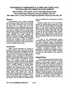
provides accurate results for all cases in which burst-level congestion is the main contributing factor of loss, which is the case for the traffic scenarios further studied. Moreover, the results obtained by Yang were checked using an ATM cell rate simulator, LINKSIM, developed by Pitts [25] and the average and maximum cell loss ratios (CLRs) obtained are used as reference values to compare the CLR predictions by ECA, FCAC and (M+1)-MMDP approximation. LINKSIM is implemented assuming that the On-Off sources considered for each of the traffic scenarios under study are independent. For each traffic scenario, the criterion for stopping the simulation is that the width of the 95% confidence interval should be less than 10% of the estimated cell loss probability. The results obtained using ECA and FCAC are plotted in figures 2. to 7. The number of sources chosen for the experiments and the link capacity values were chosen in order to get a wide range of cell loss values between 10 -2 and 10-8. The traffic sources used in the experiments are On-Off sources defined by parameters: peak and mean bit rate and mean burst length sources (see also table 1). In figure 2., the average cell loss ratio predicted by ECA is under the average cell loss curve obtained by simulation. This is because in this experiment the buffer can’t content cell level arrivals due to the large amount of active sources with relation to the small buffer size. The average cell loss ratio predicted by ECA is above the average cell loss curve obtained by simulation in figure 3., because the gain obtained by queuing part or the whole burst is ignored by the ECA approach. The ECA prediction provides an upper bound for the average cell loss probability for the traffic scenarios plotted in figures 4. and 5. ECA is conservative in this scenario being more accurate when the number of sources increases. The prediction given by the (M+1)-MMDP approach is also accurate and the accuracy increase with the average load as observed previously for a slow link (see figure 3.).

24/09/97-13

The FCAC prediction conforms with the cell loss value given by the simulation. For figure 5 the values obtained via simulations for the maximum cell loss and average cell loss vary significantly and that is the reason why FCAC predicts a more conservative value. Yang et al. describes the experiment associated with figure 4 as a traffic scenario where “burst-level congestion” is predominant and that accounts for the accuracy of the (M+1)-MMDP prediction for this traffic scenario. As we can see, for the traffic scenario studied in figure 4, the sources’ mean burst length is quite long (339 cells) and therefore, the influence on cell loss caused by queuing part of the buffer is more significant than in the case of voice traffic. The experiment associated with the results in figure 5 is described by Yang et al as the traffic scenario equivalent to the one obtained for the transfer of large files; the output buffer only copes with cell level fluctuations and all the loss is caused by lack of bandwidth resources. This constitutes a scenario for which the ECA approach is accurate. The ECA prediction for both figures 6 and 7 is below the average cell loss curve obtained via simulations but the difference is not enough to classify the prediction given by ECA as optimist. The same behaviour can be observed for the prediction given by the (M+1)-MMDP approximation. The FCAC prediction conforms with the cell loss value given by the simulation. Note that the rounding to the next power of ten can sometimes mislead the observer to think that the approach is either pessimist or optimist for a particular traffic study. For the image traffic scenarios studied in figures 6 and 7, the mean burst length is so long that the size of the buffer is not adequate to cope with fluctuations at cell level and this explains why the ECA approach does not provide an upper bound for the average cell loss value. 4.2 Heterogeneous scenarios This set of experiments allows to compare the average cell loss results obtained from on-line measurements in the Exploit ATM test-bed in Basel [26] with the cell loss

24/09/97-14

predictions given by both the ECA and FCAC approaches for heterogeneous traffic scenarios (mixes of two different traffic types) on a single ATM link. Although FCAC aims to predict the maximum cell loss ratio per connection instead of the average cell loss ratio for the aggregate traffic, for the sake of comparison with the results obtained from on-line measurements, FCAC was trained to predict the average cell loss ratio instead. In table 2 the traffic sources used for the comparison experiments are described. The link capacity considered is 155.52 Mbit/s and the output buffer size is 27 cells for all experiments in this section. Considering that the buffer size used in the ATM test-bed experiments is very small (27 cells), it is not surprising that the cell loss predicted by the convolution approach is so close to the cell loss measured values. Convolution algorithms are based on a stationary bit rate distribution and hence, the source’s mean burst length value is ignored. This implies that the cell loss prediction given by ECA is very close to the cell loss obtained for a server system with no buffers. This also explains the slight difference between the measurements curve and the convolution curve as some of the generated cells can be stored in the server output buffer, and, therefore, a more optimist cell loss is actually obtained (see measurements curve). It can also be observed from figures. 7 to 15 that the cell loss prediction given by FCAC is close to the one obtained from measurements. The fact that the cell loss predictions given by FCAC can be more optimistic than predictions given by ECA, for some traffic scenarios, has to do with the fact that the rounding-off error to the closest negative power of ten. Overall, the FCAC predictions obtained for each of the eight heterogeneous traffic mixes shown previously approximate the measurements curve and the FCAC prediction is never less optimistic and generally more optimistic than the ECA prediction.

24/09/97-15

4.3 Heterogeneous scenarios (traffic mix of five different traffic types) The traffic mixes studied in this section are composed of 6 different types of sources. All the experiments have the same background traffic composed of the sources described in table 3. The foreground traffic changes between experiments and the characteristics of the traffic sources for each experiment are described in table 4. The link configuration is the same as the one used in the experiments of the previous section, that is, the link capacity is 155.52 Mbit/s and the output buffer size is 27 cells. The sources used are VBR sources, modelled as On-Off sources and described by the peak bit rate and mean “on” and “off” periods. The cell loss ratio measurements reported in the following were possible, thanks to RACE consortium EXPLOIT made available the equipment for traffic generation and analysis at the ATM test-bed at Basel for a week of experiments (experiments C1 to C9). After this set of experiments some other were performed using an ATM cell rate simulator, LINKSIM, in order to observe the increase of the cell loss ratio for the multiplexed connections, when one more ATM-100 connection (with the same traffic characteristics as specified for the correspondent experiment) is added, each time, to the background traffic consisting of the traffic mixes studied in each of the experiments. Limitations of time and the number of connections that can be analysed by the traffic analysers at the ATM test-bed made it impossible to make this measurements on- line. The experiments will allow us to understand the influence of adding a new traffic connection (here the connection associated with the ATM-100 traffic source) on the maximum cell loss ratio to be expected for the connections. The FCAC cell loss prediction shown in figures 16 to 20 was obtained after tuning the rule base obtained for the experiments of the previous section with the measurements data collected from experiments C.1 to C.9.

24/09/97-16

Experiments C1 to C4 show the influence on the obtained cell loss ratio caused by variations on the mean burst length of the foreground traffic (ATM100 and NTUAPC7), as described in table 5. As expected, cell losses increase either because the mean-on period of the AT100 has increased or because the mean OFF period of the NTUA-PC7 has decreased (see figure 16). The ECA prediction is conservative and follows the CLR curve obtained via simulation. FCAC gives a similar cell loss prediction for experiments C1, C2 and C4 with the exception of experiment C3 for which FCAC allows to accept one more ATM100 source for a cell loss requirement of 10-4. This is expected, since experiment D3 is characterised by having the lowest load in the link of all four experiments. Experiments C2, C5 and C6 show the influence of varying the peak rate of the ATM100 traffic on the obtained cell loss ratio. As expected, decreasing the peak rate implies a decrease in the cell loss ratio also. The ECA predictions are conservative for all three experiments. The pattern of cell loss prediction given by FCAC is the same for all three experiments and this is because the variation of the total load on the link among the experiments is not such that implies different cell loss patterns. For the set of experiments defined in Table 6, the mean-on and mean-off periods of the ATM100 traffic source varies, whilst the mean-off is twice the mean-on for all the before mentioned experiments. Finally, the effect of variations of the mean burst length, keeping the mean load constant, is analysed in experiments C2, C7, 8 and C9. The mean-on and mean-off periods of ATM100 traffic vary according to table 6, maintaining the mean rate of the source constant. From figure 20, it can be observed that the duration of the mean-on and off periods have a negligible effect on the resulting cell loss ratio, for these traffic mixes. For traffic mixes with only one ATM100 source, the cell loss ratios differ slightly with variations in the duration of the bursts, as shown in figure 20.

24/09/97-17

The ECA prediction, being insensitive to variations of the size of the bursts, gives the same cell loss prediction for the four experiments. The prediction is conservative and this is due to the small number of sources and to the cell level contention carried out in the output buffer (note that mean ON period for the aggregated traffic is relatively small). FCAC is sensitive to the effect of changes in the size of the bursts but for the traffic scenario of experiments C2, C7 to C9, the influence of varying the mean burst length on the cell loss ratio is not enough to cause a different prediction pattern when increasing the number of ATM100 sources in the traffic mix.

5. Discussions on the experiments For the presented experiments, the time required for the evaluation of the CLR using the ECA algorithm has been in the order of milliseconds. Considering that the scenarios studied in the experiments contain only on-off sources, ECA’s cut-off mechanisms designed to achieve a fast evaluation of the CLR have not been applied. Therefore, the speed of the calculations can even be improved if such mechanisms are considered, which is the case in an on-line implementation of the ECA algorithm. A further improvement in the speed of calculations can be achieved considering that the CAC decision making consists of a yes/no type of answer. Hence, ECA is not required to perform the full calculations of the predicted cell loss ratio if

the partially

calculated cell loss ratio already exceeds the required cell loss ratio. The calculations stop and the new connection is rejected. The time required to perform FCAC’s calculations is also negligible. FCAC’s response is the integer corresponding to the negative integer power of ten for the cell loss ratio. This is because crisp fuzzy sets have been used for the output fuzzy variable. If bell-shaped fuzzy sets had been used instead, floating point cell loss ratios

24/09/97-18

could have been obtained but the learning algorithm would require more examples and the fuzzy inference algorithm would be slower than the current one.

6. Conclusions and Further Work The experiments described in this paper compare the cell loss ratios obtained by an “enhanced” convolution based CAC approach, ECA, with a fuzzy logic based CAC approach, FCAC. The reference cell loss ratios are obtained from measurements on an ATM link and using simulators. In order to verify the results obtained via simulation an analytical model, the (M+1)-MMDP approximation is used to calculate the cell loss ratios in case of homogeneous traffic scenarios. The cell loss predictions obtained by FCAC and ECA measurement are in agreement with the cell loss reference values obtained via on-line measurements and using simulations, although the cell loss ratio prediction given by ECA is generally conservative and the FCAC prediction is generally optimistic. The conservatism of the prediction given by ECA is related with the bufferless assumption. The optimism observed in the prediction given by FCAC is mainly related to the round-off error when rounding a floating point value of the measured cell loss ratio to the nearest negative power of ten. ECA’s algorithm is easy to be implemented. FCAC uses a learning phase based on genetic algorithms in order to define the parameters of the fuzzy logic model. The inference model is straightforward. Both ECA and FCAC can adapt to traffic patterns associated with ATM services introduced in the future. ECA only requires the definition of the peak and mean rates (on-off model) of each of the connections, but can accept a larger set of descriptive parameters (GMDP model). FCAC adaptability is only limited by the availability of

24/09/97-19

measurements for the new traffic patterns but this is not likely to constitute a problem in an on-line implementation. Future research is required to test both ECA and FCAC approaches on-line regarding the speed of the calculations, the accuracy of the cell loss ratio predictions and the optimisation of the use of the ATM link. This paper has used as much as possible results obtained from on-line measurements but the set of obtained results is not enough to make very broad conclusions. The authors regret that there isn’t a common set of ATM traffic scenarios used among ATM researchers to compare CAC approaches.

24/09/97-20

4ABLES 4RAFFIC #LASS

0EAK 2ATE -EAN 2ATE "URST ,ENGTH -BITS -BITS CELLS Voice 0.064 0.022 58 Data 10 1 339 Image 2 0.087 2604 4ABLE Traffic characteristics ([23], pp. 122).

4RAFFIC #LASS A.31 A.32 B.31 B.32 C.31 C.32

0EAK 2ATE -BITS

-EAN 2ATE -BITS

-EAN "URST , CELLS

31.1 6.22 1467 31.1 1.56 734 7.78 3.89 917 7.78 0.39 183 1.94 0.97 229 1.94 0.39 91 4ABLE Characteristics of the traffic sources.

4RAFFIC #LASS

0EAK 2ATE -EAN /N -EAN /FF -BITS PERIOD S 0ERIOD S NTUA-PC1 37 0.000836 0.00336 NTUA-PC2 37 0.00126 0.00293 NTUA-PC3 37 0.00167 0.006715 NTUA-PC4 37 0.00252 0.005878 4ABLE Traffic characteristics for the background traffic.

24/09/97-21

Experiment

C1 C2 C3 C4 C5 C6 C7 C8 C9

Peak Rate (Mbit/s) 37 37 37 37 37 37 37 37 37

NTUA-PC7 Mean On Mean Off Period (s) Period (s) 0.007975 0.007975 0.007975 0.007975 0.007975 0.007975 0.007975 0.007975 0.007975

0.007975 0.007975 0.009568 0.009568 0.007975 0.007975 0.007975 0.007975 0.007975

Peak Rate (Mbit/s) 8 8 8 8 7 6 8 8 8

ATM-100 Mean On Mean Off Period (s) Period (s) 0.02 0.04 0.02 0.04 0.04 0.04 0.02 0.06 0.01

0.08 0.08 0.08 0.08 0.08 0.08 0.04 0.12 0.02

4ABLE Traffic characteristics for the foreground traffic (experiments C1 to C9) !4- -EAN OFF Mean-on = 0.02 Mean-on = 0.04 Mean-off = 0.007975 Exp. C1 Exp. C2 .45! 0# Mean-off = 0.009568 Exp. C3 Exp. C4 -EAN ON 4ABLE Structure of experiments C1 to C4 varying the characteristics ATM100 and NTUA-PC7. %XPERIMENT 0EAK -EAN ON S -EAN OFF S C9 8 0.01 0.02 C7 8 0.02 0.04 C2 8 0.04 0.08 C8 8 0.06 0.12 4ABLE Structure of experiments C2, C7, C8 and C9 for which the mean load is kept constant but the mean on and off periods of the ATM-100 traffic source vary.

24/09/97-22

&IGURES CSV1

CSV0 sk

s0

CSVL-1

SMXL-1

Multinomial.

SMX0

SMX1 One-element Multi-Convolution.

Final SSV

&IGURE /VERVIEW OF THE %NHANCED #ONVOLUTION !PPROACH FCAC

Simul.

1,E-01

1,E-01

1,E-02

1,E-02

2,1,E-03 #1,E-04

1,E-03 2 ,# 1,E-04

1,E-05

1,E-05

!4- S OURCE S

&IGURE 6OICE calls (C=7Mbit/s, K=50)

MMDP

25

23

21

19

1,E-06 15

300

290

280

270

260

250

1,E-06

ECA

17

Legends for Figures 2 to 8

!4- S OURCE S

&IGURE 6OICE calls (C = 0.7Mbit/s and K=50)

24/09/97-23

1,E-01

1,E-01

1,E-02

1,E-02

2,1,E-03 #1,E-04

1,E-03 2 ,# 1,E-04

1,E-05

1,E-05 25

22

18

15

12

8

!4- S OURCE S

10

1,E-06

300

280

260

240

220

200

180

160

1,E-06

!4- S OURCE S

&IGURE . $ATA calls (C = 350 Mbit/s and K=50)

&IGURE $ATA calls (C = 52 Mbit/s and K=50

1,E-01

1,E-01

1,E-02

1,E-02

2,1,E-03 #1,E-04

1,E-03 2 ,# 1,E-04

1,E-05

1,E-05

1,E-06

1,E-06 80

113

150

187

220

4

!4- S OURCE S

8

12

18

22

!4- S OUR CE S

&IGURE )MAGE calls (C = 30 Mbit/s and K=50)

Legends for Figures 9 to 20

&IGURE )MAGE calls (C = 7 Mbit/s and K=50)

FCAC

1,E-01 1,E-02 21,E-03

ECA

Simul

1,E-01 1,E-02 2,1,E-03 #1,E-04 1,E-05 1,E-06

,# 1,E-04

14

24

20

16

12

8

6

1,E-05 1,E-06 .UM BE R !4- S OURCE S

&IGURE CLR (4 A.31, variable # B.31).

18

26

30

.UM BE R !4- S OURCE S

&IGURE CLR (2 A.31, variable # B.31)

24/09/97-24

1,E-02 1,E-02

21,E-04 ,# 1,E-06

2,1,E-04 #

1,E-08

1,E-08 .UM BE R !4- S OURCE S

230

190

170

150

130

74

160

140

100

80

60

20

1,E-06


&IGURE CLR (4 A.31, variable # B.32)

&IGURE CLR (2 A.31, variable

# B.32

1,E-02

1,E-02

2,1,E-04 #

2,1,E-04 #

1,E-08

1,E-08

1,E-01

1,E-02

2,1,E-03 #1,E-05

1,E-04 1,E-05

100

80

&IGURE . CLR (4 A.31, variable # C.31)

1,E-01

2, #1,E-03

70



&IGURE CLR (2 A.31, variable # C.31)

60

120

50

100

40

80

32

70

24

1,E-06

1,E-06

1,E-07 120

140

80


&IGURE CLR (4 B.3.1, variable # C.31) FCAC

100

120


&IGURE CLR (8 B.3.1, variable # C.31)

ECA

24/09/97-25

Simul

The mean-ON period of the ATM-100 source increases 1,E-02

1,E-02

1,E-03 ,# period of the 2 1,E-04 NTUA-PC7 1,E-05

2,1,E-03 #1,E-04

The mean-OFF

1,E-05 1

source

2

3

4

5

1

.UM BE R !4- S OUR CE S

2

3

4

5


decreases Cell loss Predictions for experiment C3. Cell loss Predictions for experiment C4.

1,E-02

1,E-02

1,E-03 2 ,# 1,E-04

2,1,E-03 #1,E-04

1,E-05

1,E-05 1

2

3

4

5

1


2

3

4

5


Cell loss Predictions for experiment C1. Cell loss Predictions for experiment C2. &IGURE Cell loss predictions for experiments C1 to C4. 1,E-02

1,E-02

1,E-03 2 ,# 1,E-04

2,1,E-03 #1,E-04

1,E-05

1,E-05 1

2

3

4

5

1


2

3

4


&IGURE Cell loss Predictions Exp. C2

&IGURE Cell loss Predictions Exp. C5

1,E-02 1,E-03 2 ,# 1,E-04

FCAC

1,E-05 1

2

3

4


&IGURE Cell loss Predictions for experiment C6

24/09/97-26

ECA

Simul

1,E-02

2, 1,E-03 # 1,E-04 1,E-05 1

2

3

4

5


FCAC

ECA

Simul2

Simul7

Simul8

Simul9

&IGURE Comparative Cell loss ratio predictions for experiments C2, C7, C8 and C9 .

24/09/97-27

6.1 References

[1 [2] ITU Rec. I.121, “Broadband aspects of B-ISDN”, Rev. 1, Geneva, 1991. [3] H. Saito H., “Call admission control in an ATM network using upper bound of cell loss probability”, IEEE Transactions on Communications vol. 40 n. 9 (1992). [4] ITU, Rec. I. 371, Study Group 13, “Traffic Control and Congestion Control in B-ISDN”, Geneva, 1995. [5] W. Stallings, “ISDN and B-ISDN with Frame Relay and ATM”, PrenticeHall, 1995. [6] R.O. Onvural, “Asynchronous Transfer Mode Networks: Performance Issues”, Artech House, Boston, London, 1994. [7] J.Y.Hui, "Resource Allocation for broadband networks", IEEE J. on Sel. A. in Com., vol. SAC-6, no.9, pp. 1598-1608, Dec. 1988. [8] R. Guerin, H. Ahmadi, M. Naghshineh, "Equivalent capacity and its application to bandwidth allocation in high-speed networks", IEEE J. on Sel. areas in com., vol. 9, no.7, Sept. 1991. [9] V.B. Iversen and Liu Y., "The performance of convolution algorithms for evaluating the total load in an ISDN system”, 9th Nordic Teletraffic Seminar, Norway, pp. 14, Aug. 1990. [10] J.L.Marzo, R. Fabregat, J. Domingo, J. Sole. "Fast Calculation of the CAC Convolution Algorithm, using the Multinomial Distribution Function". Tenth UK Teletraffic Symposium, pp.23/1-23/6, 1993.

24/09/97-28

[11] M. F. Ramalho and E. M. Scharf, "Developing a Fuzzy Logic Tool using Genetic Algorithms for Connection Admission Control in ATM Networks", Proc. of the 6th Int’l Fuzzy Systems Association World Congress, Vol. 1, pp. 281-284, S. Paulo, 22-28th July 1995. [12] R.Fabregat-Gesa, J. Sole-Pareta J.L.Marzo-Lazaro, J. Domingo-Pascual, “Bandwidth Allocation Based on Real Time Calculations Using the Convolution Approach”, Globecom 1994. [13]

R.Fabregat-Gesa,

J.L.Marzo-Lazaro

and

Pere

Ridao,

”Resource

dimensioning aspect of heterogeneous traffic with different service requirements: integration versus segregation" Twelfth UK Teletraffic Symposium, Windsor. [14] RACE. “Updated Results of Traffic Simulation of the Policing Experiments”. Technology for ATD. December 1990. [15] “Updated Results of Traffic Simulation of the Policing. Experiment R1022.Technology for ATD. 1990. [16] T. Takahashi, A. Hiramatsu, “Integrated ATM traffic control by distributed neural networks”, in Proc. ISS ’90, Stockholm, vol. 3, pp. 59-65, 1990. [17] M. Fontaine and D.G. Smith, “A neuro-fuzzy approach to connection admission control in ATM networks”, 13th UKTS, Glasgow, 1996, session 1, paper 2, pp. 2/1 to 2/8. [18] T. Worster, "Neural network based Controllers for Connection Acceptance", 2nd RACE Workshop on Traffic and Performance Aspects in IBCN, Aveiro, Portugal, Jan., 1992. [19] K. Kosko, "Neural Networks and Fuzzy Systems: a dynamical systems approach to Machine Intelligence", Prentice Hall International Editions, 1992.

24/09/97-29

[20] Herrera F., Lozano M., Verdegay J., “A learning process for Fuzzy Control rules using Genetic Algorithms”, Dept. of Computer Science and Artificial Intelligence, Univ. Granada, Spain, Technical Report #DECSAI-95108, February 1995. [21] M. F. Ramalho and E. M. Scharf, “Fuzzy Logic Tool and Genetic Algorithms for CAC in ATM Networks” in Electronic Letters, vol. 32, no. 11, pp. 973-974, 1996. [22] M. F. Ramalho and E. M. Scharf, “The application of Fuzzy Logic Techniques and Genetic Algorithms for Connection Admission Control in ATM Networks”, in: Genetic Algorithms and Soft Computing, F. Herrera, J.L. Verdegay (Eds.), Physica-Verlag (Studies in Fuzziness, Vol. 8), pp. 615-640, 1996. [23] Kim Chwee Ng, Yun Li, “Design of Sophisticated Fuzzy Logic Controllers Using genetic Algorithms”, Proc. 3rd IEEE Int. Conf. on Fuzzy Systems, IEEE World Congress on Computational Intelligence, Orlando FL, June 1994, vol. 3, pp. 1708-1712. [24] T. Yang, D.H.K. Tsang, “A novel approach to estimating the Cell Loss Probability in an ATM Multiplexer loaded with Homogeneous On-Off sources”, IEEE Trans. on Communications, vol. 43, no.1, pp. 117-126, January 1995. [25] Pitts J.M., "Cell-rate simulation modelling of Asynchronous Tranfer Mode Telecommunications Networks", Ph.D. Thesis, Queen Mary and Westfield College, July 1993. [26] EXPLOIT-RACE2061/EXP/SW3/DS/P/028/B1, “Results of Experiments on Traffic Control using Real Applications”, 31 December 1994.

24/09/97-30