The energy release rate was also evaluated using linear elastic ... Linear elastic fracture mechanics, Fiber reinforced polymer, strain energy release rate.
Rev. Téc. Ing. Univ. Zulia. Vol. 37, Nº 2, 1 - 9, 2014
Determining the crack propagation in DCB composite specimens by fiber bridging modeling A.Kaveh University of Science and Technology, Tehran, Iran
Abstract-This paper employs the experimental and FEA analysis for determine the crack mode opening displacement(CMOD) and energy release rate(ERR) of the laminated composites under mode I loading was studied using the double cantilever beam test. The energy release rate was also evaluated using linear elastic fracture mechanics (LEFM) and FEA analysis in ANSYS software. The results obtained using the above two techniques are found to be in good agreement. Keywords: Linear elastic fracture mechanics, Fiber reinforced polymer, strain energy release rate. 1 INTRODUCTION Due to their great potential in weight saving, laminated composites are becoming increasingly important in applications where low weight, high stiffness and high strength is required. Laminated fiber reinforced polymer composites have attracted a wide range of uses in civil, marine, automotive, aerospace and sports applications on account of their superior tailor made properties that are not attainable from conventional metallic materials. However composites made of laminates exhibit a worrying susceptibility to the appearance and growth of cracks between the layers. This phenomenon is known as delamination which is one of the critical damage mode that limits laminated composite‟s load-carrying capability. The technological causes of delamination can be grouped into two categories. The first category includes delamination due to curved sections, such as curved segments, tubular sections, cylinders and spheres, and pressurized containers. Delamination due abrupt changes of section such as ply drop-offs, union between stiffeners and thin plates, free edges, and other bonded and bolted joints. Although several decades have passed since the recognition of the importance of interlaminar failure, it still remains a determining factor limiting the use of structural elements made of laminated composites. Hence, reliable measure of delamination resistance is essential in the design of fiber composites. Linear elastic Fracture Mechanics (LEFM) is suitable for predicting delamination growth. Fracture toughness is a property which describes the ability of a material containing a crack to resist fracture. Stress intensity factor is the general parameter defining the fracture toughness of materials. For analysing the interlaminar fracture of composites this concept is difficult to apply as different anisotropic properties are present above and below the plane of delamination. In this paper fracture toughness is evaluated based on Energy release rate (ERR) using Linear elastic Fracture Mechanics (LEFM). 2 EXPERIMENTAL WORK The experimental work was executed by two steps. They are fabrication work and testing work. In the fabrication work the three different layers or thickness Epoxy/fiber glass composite material was manufactured and machined two different length specimens. Then the fixtures are manufactured and fixed the fixtures in the two width of the double cantilever test specimen‟s one end. The initial crack was precut by a diamond saw of thickness one millimeter. The crack tip was sharpened by a thin blade to extend the initial crack length. Then the test specimens were set curing for the particular period at the atmospheric conditions. In the testing work the prepared test specimens were loaded by a wedge load under displacement control with a constant speed in automated tensile testing machine. The fiber bridging was created. The load displacement curve and the displacement at the particular load data were observed. In the fabrication work first the unidirectional glass fiber (900 GSM) sheets were cut as per the required size. The size of the sheets were as follows 1. 93 cm × 50 cm - 3sets 2. 63 cm × 50 cm - 3sets 3. 33 cm × 50 cm - 3sets Now the work table was cleaned and the wax coated over the table. Then the epoxy resin was taken as per the volume fraction ratio (65% glass fiber: 35% epoxy resin). Then added the hardener as the standard ratio of 1:10 and stir well to mix the hardener and the resin to achieving the jell condition. Now the jelly paste was coated over the table and the 93 cm length sheet was layup the coated jelly. Then the jelly was coated over the first layer and sweep uniformly throughout its length. Similarly the three layers were produced. Then the 63 cm 33cm length sheets were lay up from the one end of the three layers as from the above manner. Then the three different layers wetted composite was solidified and cured for seven days in the atmospheric condition. Then the cured sheets were cut as the required test specimen sizes with the help of power hand saw cutting machine. Then
1
Rev. Téc. Ing. Univ. Zulia. Vol. 37, Nº 2, 1 - 9, 2014
the test pieces were accurately machined by the fine abrasive grinding machine. The test specimens are as following, 1.
100 mm × 30 mm
- 3pieces (3, 5 & 7 layers)
2.
200 mm × 30 mm
- 3pieces (3, 5 & 7 layer)
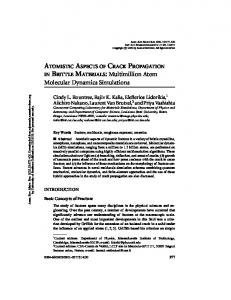
Then the fixtures for clamping the one end of the DCB test specimens were manufactured using the carped glass fibers/epoxy and fixed the fixtures in the two width of the double cantilever test specimen‟s one end. Then it allowed curing for few days. After cured the fixtures the initial crack was precut by a diamond saw of thickness one millimeter in the centre of the test specimen‟s fixtures end. Then the crack tip was sharpened by a thin blade to extend the initial crack length up to 25 mm. Now the different layer and different length DCB glass fiber/epoxy unidirectional composite specimens were fabricated and ready for testing. The testing process was conducted in the Mechanical Test Lab of Central Institute of plastics Engineering & Technology (CIPET) Chennai. There the DCB unidirectional glass fiber /Epoxy composite test specimens were tested by a Autograph AG -IS tensile testing machine. This machine was standard high precision universal testing machine. It has the automatic result software and the automatic graph plotter. Its crosshead speed range 0.001 to 1000 mm/minute for load range up to 50 KN capacity load cell. The test specimens were loaded by a wedge load under displacement control with a constant speed of 1 mm/min. Then the crack was propagated and the fiber bridging was formed exactly. Then observe the load displacement curve in the desktop linked with the testing machine. In this procedure the test was conducted and the test results were used to calculate the energy release rate (G). 3 DATA REDUCTION SCHEME Energy release rate is defined as energy release per unit increase in area during crack growth. It is denoted by the symbol G. The most common approach to delamination analysis is the calculation of the strain energy release rate, SERR, based on linear elastic fracture mechanics, LEFM. This method is limited to “brittle matrices”; for tough matrices, another method like elastic-plastic fracture mechanics may be employed, i.e., Jintegral. Energy release rate (G) is a measure of how tough the material is in resisting delamination and can be calculated from the load-deflection curve. The geometry of a DCB specimen is shown in Fig.1where h is the thickness of the specimen, which was varied, 𝑎𝑜 is an initial notch, 𝑎 is the length of a propagated crack, d is the crack opening under the applied wedge forces P, and 𝛿 ∗ is the crack opening at the tip of the initial notch. The description of the loading and measurement method is given in the experimental part.
Fig.1 The geometry of a DCB specimen The energy release rate in a DCB specimen is defined in a usual way: ∂П G= (1) b ∂a Where b is the width of the specimen, 𝑎 is the crack length, П is the potential energy accumulated in the system, and P is the force by which both sides of the specimens are loaded. The potential energy of a linearly elastic system is equal to 1 П= 2
u
u
ζij εij dv − v
P u du
( 2)
0
Where 𝜎𝑖𝑗 and 𝜀𝑖𝑗 are the stress and strain, V is the volume, 𝑃 𝑢 is the force applied, which is the function of displacement. The first term is an energy stored in the linearly elastic body and the second one is the work produced by the applied external force. The displacement u is a full opening of the DCB specimen at the point where P is applied. The first term is also expressed through the force acting on the system 1 П = Pu − 2
u
P u du
(3)
0
2
Rev. Téc. Ing. Univ. Zulia. Vol. 37, Nº 2, 1 - 9, 2014
Then we determine the energy release rate from Equations (1) and (3) it follows that 1 ∂P 1 ∂u 1 ∂u 1 ∂u ∂P G= u− P + P = P − u 2b ∂a 2b ∂a b ∂a 2b ∂a ∂a or p 2 ∂c
G= (4) 2b ∂a Here c is the compliance. The formula (4) is well-known and widely used. Note that no assumptions about the type of the crack tip structure was made, therefore the formula (4) is general and should be valid for any bridging and specimen shape. But the G values obtained can functions of the specimen shape, not only the characteristics of the material. G depends on the compliance 𝑐 = 𝑢 𝑃 , which is measured experimentally or calculating theoretically using some bridging law.The deflection of an ideal cantilever beam, with cracked length 𝑎 and bending stiffness EI = 𝐸𝑏ℎ3 12 under a load P is equal to 𝑎3 𝑃 3𝐸𝐼 . The full opening of the DCB equals the doubled deflection, 2𝑎 3 𝑃
𝑢= 𝑑=
(5)
3EI
and the compliance is c = 2a 3
u p
c= (6) 3EI Now using equation (4) and (6) we get the most popular formula for energy release rate of the DCB specimen is obtained. This formula is use to determine the energy release rate (G) value from the results of load (P) and propagated crack length (𝑎). G=
p2
×
2b
∂c
∂a P2a2
=
p2
×
2b
2×3a 2 3EI
G P,a = (7) EIb Combining equations (7) and (5), we get three another modified formulae for energy release rate G 𝑑=
2𝑎 3 𝑃
3EI 3𝐸𝐼𝑑
𝑎2 = 2𝑃𝑎 Substitute the value of 𝑎2 into equation (7) we get the first modified formula for energy release rate (G) value from the results of load (P), propagated crack length (𝑎) and crack mouth opening displacement (d) . P2
G P,a,d =
EIb 3Pd
×
3EId 2Pa
G P,a,d = 2ab Then we get the second modified formula for energy release rate (G).From the equation (5) 3EId a3 = 2P
a=
1
3EId 2P
𝟑𝑬𝑰𝒅
(8)
3 𝟐
𝟑
𝒂𝟐 = 𝟐𝑷 Substitute the value of 𝑎2 into equation (7) we get the second modified formula for energy release rate (G) value from the results of load (P) and crack mouth opening displacement (d). P2
3EId
2
3
G P,d = EIb 2P Finally we get the second modified formula for energy release rate (G).From the equation (5) 3EId P= 3
(9)
2a
Substitute the value of P into equation (7) we get the third modified formula for energy release rate (G) value from the results of propagated crack length (𝑎) and crack mouth opening displacement (d) G a,d = G a,d =
3EId 2a 3 9EI d 2 4a 4 b
×
3EId 2a 3
×
a2 EIb
(10)
G value calculated directly from finite element analysis results with the formulas (7) – (10), they conclude, that formula (9) performs better 1 . In our case the crack mouth opening displacement (CMOD) d and the corresponding load P are obtained from the experimental testing result and finite element analysis results. Therefore we used the formula (9) to determine the energy release rate (G) for both FEA and experiment.
3
Rev. Téc. Ing. Univ. Zulia. Vol. 37, Nº 2, 1 - 9, 2014
4 FINITE ELEMENT METHOD Finite element analysis is an effective numerical method in which the given domain of interest is subdivided into discrete shapes called elements which form an inter-connecting network of concentrated nodes. The material properties and governing relations are considered over these elements and expressed in terms of unknown values at element corners. An assembly process duly considering the loading and constrains results in the set of equations. Solutions of these equations give the approximate behaviour of the continuum. Determining the interrelating behaviours of all the nodes the system, the behaviour of the entire object can be assessed. The entire object can thus be analyzed for stress-strain, heat transfer and other characteristics by calculating the behaviour of each node. In this work ANSYS 11.0 finite element software, which has the post processing capabilities to determine fracture parameters like the stress factor (K), J-integral, Energy Release (G) and Crack Tip Opening Displacement (CTOD) is used for the analysis. One of the methods employed in evaluation of Crack Tip Opening Displacement (CTOD) is cohesive zone modeling technique in which the cohesive zone will be modelled ahead of crack tip. In this problem, element type PLANE182 is used for a 2-D fracture model. PLANE182 is a higher order version of the 2-D, four node element. It provides more accurate results for mixed (quadrilateral- triangular) automatic meshes and can tolerate irregular shapes without as much loss of accuracy. The 8-node elements has compatible displacement shapes and are well suited to model curved boundaries.
Fig.2 Plane 182 Elements The element may be used as a plane element or as an axi-symmetric element. The Element has plasticity, creep, swelling, stress stiffening, large deflection and large strain capabilities. The Row of elements around the crack tip should be singular as shown in figure 3
Fig.3 Singular Elements The fracture mechanics based approach can be used for sharp crack of linear elastic materials to study the problems. As to the energy based criterion (strain energy release rate, SERR), the virtual crack closure technique (VCCT) is powerful tool to compute SERR by using finite element analysis (FEA). Some applications of VCCT to study the crack growth can be found. However, in reality, neither the idealized sharp crack nor the linear elastic material does exist. This is particular true for composite materials and adhesively bonded joints. Therefore, recently, using of cohesive zone model (CZM) is increasing. The idea of CZM is straightforward. It is a natural extension of BD model, which was proposed for perfect plastic materials. However, the implementation of CZM with FEA varies. There are two major classes: continuum cohesive zone model (CCZM) and discrete cohesive zone model (DCZM).Fracture or delamination along an interface between phases plays a major role in limiting the toughness and the ductility of the multi-phase materials, such as matrix- matrix composites and laminated composite structure. This has motivated considerable research on the failure of the interfaces. Interface delamination can be modeled by traditional fracture mechanics methods such as the nodal release technique. Alternatively, you can use techniques that directly introduce fracture mechanism by adopting softening relationships between tractions and the separations, which in turn introduce a critical fracture energy that is also the energy required to break apart the interface surfaces. This technique is called the cohesive zone model. The interface surfaces of the materials can be represented by a special set of interface elements or contact elements, and a cohesive zone model can be used to characterize the constitutive behavior of the interface. The cohesive zone model consists of a constitutive relation between the traction T acting on the interface and the corresponding interfacial separation δ (displacement jump across the interface). The definitions of traction and separation depend on the element and the material model. The cohesive model has been
4
Rev. Téc. Ing. Univ. Zulia. Vol. 37, Nº 2, 1 - 9, 2014
formulated such that it can be used for practical application. Cohesive zone model is widely utilized in engineering to predict various behaviors such as the crack propagation in the interface of the two materials, fatigue crack propagation and the delimitation in the composite materials. Cohesive zone model can be represented in Finite Element Analysis with the help of some software packages. ANSYS is the software which is used in this paper work to model the cohesive zone in the test specimen. Interface elements representing the damage are implemented between the continuum elements representing the elastic plastic properties of the material. Several investigations deal with the effect of the shape of the traction–separation function on the resulting fracture behavior. Here the normal separation traction can be found out by using the formula given as follows. δ − δ2 3 δ − δ2 2 T = T0. 2 −3 +1 (11) δ0 − δ2 δ0 − δ2 Due to the simple geometry, the hybrid technique using a finite element analysis is not needed: the applied force at fracture is divided by the instantaneous cross section as in a thin flat tensile specimen a uniform stress state can be assumed. The flow stress of the material can also be used as this traction separation stress. Cohesive zone can be modeled in ANSYS by using interface elements. Inter 202 is the suitable interface element for continuum element Plane 182 which is used to mesh the areas around the cohesive zone. Initially, geometry with given dimension has to be modeled. One interface element and a continuum element have to be selected where interface element is used to define cohesive zone and continuum element is used to describe the elements around the cohesive zone. A Local coordinate system is created at the crack tip. Crack tip is modeled with singular element by using concentrated key point. Cohesive zone properties are defined by calculating the flow stress of the material. Cohesive zone is meshed ahead of crack tip throughout the ligament area. Mode I debonding defines a mode separation of the interface surface where the separation normal to the interface dominates the slip tangent to the interface. The normal contact stress (tension) and contact gap behavior is plotted in figure 5.7. It shows linear elastic loading (OA) followed by linear softening (AC). The maximum normal contact stress is achieved at point A. Debonding begins at point A and is completed at point C when the normal contact reaches zero value, any further separation occurs without any normal contact stress. The area under the curve OAC is the energy released due to the debonding and is called the critical fracture energy. Table 1 Material Properties for unidirectional fiber glass/epoxy composite. Properties Unidirectional Glass Fiber/Epoxy Composite 59GPa EXX Young‟s 20GPa EYY modulus(E) 20GPa EZZ 0.26 νXY Poisson‟s ratio(ν) 0.28 νYZ 0.26 νXZ 9GPa GXY Shear modulus(G) 1.9GPa GYZ 9GPa GXZ In the pre-processor stage, first the material curve is generated using material properties, poison ratio and Young‟s modulus as per table 5.1. The element types used here are single 2-D, 4-node structural solid (plane 182) and 2-D, 4 node Cohesive zone (Inter 202). The numbers of layer is given in the form of Main menu > Preprocessor> sections > shell> layup> add/edit> add > orientation. In the modeling stage, full portion of the specimens is modeled using key points, lines and areas. The cracked DCB specimen is modeled and the crack is modeled by using concentrate key point method as shown in figure 5.8. The model is meshed with two elements which are PLANE 182 and INTER 202.
5
Rev. Téc. Ing. Univ. Zulia. Vol. 37, Nº 2, 1 - 9, 2014
Fig.4 Deformed shape of DCB specimen
LOAD (N)
5 RESULTS AND DISCUSSION The numerical analysis on delamination of DCB specimen of Epoxy/glass fiber unidirectional composite has been carried out by using the finite element software ANSYS. The specimen is taken in three different thickness and length. Cohesive zone is modeled in the specimen ahead of artificially introduced crack to simulate the fiber bridging. The considered geometrical dimensions of the specimen are as follows 1. 3 layer, 3.9 mm thick, 30mm width and 100 & 200 mm length specimens. 2. 5 layer, 6.8 mm thick, 30mm width and 100 & 200 mm length specimens. 3. 7 layer, 9.15 mm thick, 30mm width and 100 & 200mm length specimens. 160 140 120 100 80 60 40 20 0
Load Vs CMOD (3 Layers)
0.00
5.00
100 mm FEA
200 mm FEA
100 mm EXP
200 mm EXP
10.00
15.00
20.00
25.00
30.00
CMOD (mm) Fig.5 Relation between load and CMOD for 3 layers
LOAD (N)
Load Vs ERR(G) (3 Layers) 160 140 120 100 80 60 40 20 0 0.00
100.00
200.00
300.00
100 mm FEA
200 mm FEA
100 mm EXP
200 mm EXP
400.00 500.00 ERR(J/m²) Fig.6 Relation between load and ERR for 3 layers
600.00
700.00
800.00
900.00 1000.00
6
Rev. Téc. Ing. Univ. Zulia. Vol. 37, Nº 2, 1 - 9, 2014
350 Load Vs CMOD (5 Layers)
300
LOAD (N)
250 200 150 100
100 mm FEA 100 mm EXP
50
200 mm FEA 200 mm EXP
0 0.00
5.00
10.00
15.00
20.00
25.00
CMOD (mm) Fig.7 Relation between load and ERR for 5 layers
350
Load Vs ERR(G) (5 Layers)
300
LOAD (N)
250 200 150 100 50
100 mm FEA
200 mm FEA
100 mm EXP
200 mm EXP
0 0.00
100.00 200.00 300.00 400.00 500.00 600.00 700.00 800.00 900.00 1000.00 ERR(J/m²)
Fig.8 Relation between load and ERR for 5 layers
Load Vs CMOD (7 Layers)
500
LOAD (N)
400 300 200 100 mm FEA
200 mm FEA
100 mm EXP
200 mm EXP
100 0 0.00
5.00
10.00
15.00 20.00 CMOD (mm) Fig.9 Relation between load and CMOD for 7 layers
25.00
30.00
35.00
7
Rev. Téc. Ing. Univ. Zulia. Vol. 37, Nº 2, 1 - 9, 2014
450
Load Vs ERR(G) (7 Layers)
400
LOAD (N)
350 300 250 200 150 100
100 mm FEA
200mm FEA
50
100 mm EXP
200 mm EXP
0 0.00
200.00
400.00
600.00
800.00
1000.00
1200.00
1400.00
ERR(J/m²) Fig.10 Relation between load and ERR for 7 layers Figure 8, 10 and 12 shows that when the applied load is increased the crack mouth opening displacement (CMOD) is increased. And also when the thickness and the length of the specimen are increased, load requirement for the crack mouth opening is increased due to the resistance offered by the material. Figure 9, 11 and 13 shows that when applied load is increased, energy release rate is increased initially and then reached a constant value at a point of load. And also when thickness and the length of the material increased, load requirement for the energy release is increased due to the resistance offered by the material. 5 CONCLUSION The specimens of the different layers (3layers, 5layers and 7layers) and lengths (100 mm and 200 mm) of unidirectional DCB Epoxy-glass fiber composite material are fabricated. Artificial crack is created in the middle layer of the specimens. The crack propagation of the unidirectional DCB Epoxy-glass fiber composite specimens was experimentally tested with fiber bridging. Then the crack propagation analyses on unidirectional DCB Epoxy-glass fiber composite specimens were numerically done by using ANSYS software with fiber bridging modeling. The CMOD value of the different layers or thickness and different length material for varying loading condition is obtained both experimentally and numerically. The energy release rate of the material with different thickness and different length is obtained by using the theoretical formula derived. Then the results are compared. ACKNOWLEDGEMENT We would like to express our deep sense of gratitude and respect to Management, Principal and all staff members of mechanical Engg Dept., Caarmel Engineering college and Mr.S.John Britto, Asst. Prof, Sardar Raja College of Engineering,Tirunelvelli, for their excellent guidance, suggestions and constructive criticism. We are very thankful to the Management and the Principal of Sardar Raja College of Engineering,Tirunelvelli for providing all facilities to conduct our work. References Ahmed Elmarakbi, “Finite Element Analysis Of Delamination Growth In Composite Materials Using Ls-Dyna: Formulation And Implementation Of New Cohesive Elements” Advances in Composites Materials - Ecodesign and Analysis, Pp 409 – 428. Andras Szekrenyes, Jozse Uj, “advanced Beam model for fiber-bridging in unidirectional composite double cantilever beam specimens” Engineering Fracture Mechanics 72 (2005), pp2686-2702. Bent F. Sorensen, E. Kristofer Gamstedt, Rasmus C. Ostergaard, and Stergios Goutianos, „micromechanical model of cross over fiber bridging prediction of mixed mode bridging laws‟, Mechanics Of Material 40 (2008) pp220-234. H. Sun, S. Rajendran and D. Q. Song, „Finite Element Analysis on Delamination Fracture Toughness of Composite Specimens‟, Proceedings Of 2nd Asian ANSYS User Conference, Nov 11-13, 1998, Singapore, pp 1-8. K. R. Pradeep, B. Nageswara Rao, S. M. Sivakumar and K. Balasubramanium, „Interface Fracture Assessment on Sandwich DCB Specimens‟, Reinforced Plastics and Composites, Vol. 29, No 13/2010, Pp 1963-1977. Kyongchan Song, Carlos G. Davila, Cheryl A. Rose, „Guidelines and Parameter Selection for the Simulation of Progressive Delamination‟, Abaqus Users‟ Conference, 2008, Pp 1-15. 8
Rev. Téc. Ing. Univ. Zulia. Vol. 37, Nº 2, 1 - 9, 2014
Lee J.H., Wang H., Korjakin A. and Richard H.A. “Investigation of mixed Mode I/II interlaminar fracture toughness of laminated composites by using a CTS type specimen”. Engineering Fracture Mechanics, Vol. 61, Pp 325-342, 1998. M. Nikbakht, and N.Choupani “Fracture Toughness Characterization of Carbon-Epoxy Composite using Arcan Specimen” International Journal of Aerospace and Mechanical Engineering 2:4 2008, Pp 247 – 253. Tamuzs V, Tarasovs S, and Vilks U. “Progressive delamination and fiber bridging modeling in double cantilever beam composite specimen” Engineering Fracture Mechanics 68 (2001), pp513–525.
9